| Issue |
A&A
Volume 552, April 2013
|
|
|---|---|---|
| Article Number | L8 | |
| Number of page(s) | 4 | |
| Section | Letters | |
| DOI | https://doi.org/10.1051/0004-6361/201321194 | |
| Published online | 29 March 2013 | |
Physical properties of outflows⋆
Comparing CO- and H2O-based parameters in Class 0 sources
1
Department of Earth and Space SciencesChalmers University of Technology,
Onsala Space Observatory,
439 92
Onsala,
Sweden
e-mail:
This email address is being protected from spambots. You need JavaScript enabled to view it.
2
INAF – Osservatorio Astronomico di Roma, via di Frascati
33, 00040
Monte Porzio Catone,
Italy
3
Observatorio Astronómico Nacional (IGN),
Calle Alfonso XII, 3.,
28014
Madrid,
Spain
4
Onsala Space Observatory, Chalmers University of
Technology, 439
92
Onsala,
Sweden
5
Harvard–Smithsonian Center for Astrophysics, 60 Garden
Street, Cambridge,
MA
02138,
USA
Received: 30 January 2013
Accepted: 7 March 2013
Abstract
Context. The observed physical properties of outflows from low-mass sources put constraints on possible ejection mechanisms. Historically, these quantities have been derived from CO using ground-based observations. It is, therefore, important to investigate whether parameters such as momentum rate (thrust) and mechanical luminosity (power) are the same when different molecular tracers are used.
Aims. Our objective is to determine the outflow momentum, dynamical time-scale, thrust, energy, and power using CO and H2O as tracers of outflow activity.
Methods. Within the framework of the Water In Star-forming regions with Herschel (WISH) key program, three molecular outflows from Class 0 sources have been mapped using the Heterodyne Instrument for the Far Infrared (HIFI) instrument aboard Herschel. We used these observations together with previously published H2 data to infer the physical properties of the outflows. We compared the physical properties derived here with previous estimates based on CO observations.
Results. Inspection of the spatial distribution of H2O and H2 confirms that these molecules are co-spatial. The most prominent emission peaks in H2 coincide with strong H2O emission peaks and the estimated widths of the flows when using the two tracers are comparable.
Conclusions. For the momentum rate and the mechanical luminosity, inferred values are not dependent on which tracer is used, i.e. the values agree to within a factor of 4 and 3, respectively.
Key words: ISM: molecules / ISM: jets and outflows / stars: formation / stars: winds, outflows
Herschel is an ESA space observatory with science instruments provided by European-led Principal Investigator consortia and with important participation from NASA.
© ESO, 2013
1. Introduction
The emission from CO is a widely used tracer of outflow activity. The lowest rotational transitions emit photons in the millimetre and sub-millimetre part of the electromagnetic spectrum making CO relatively straightforward to observe using ground-based telescopes. This, and the abundance of CO with respect to molecular hydrogen, has led to extensive mapping campaigns that cover entire outflows during the last two decades. Rotational transitions of H2O and H2 are, on the contrary, not easily observed from the ground and recent observations have primarily relied on the use of space-based telescopes (e.g. ISO, SWAS, and Odin). However, the limited achievable spatial resolution on these missions hampered the interpretation of the data. The situation has improved since the launch of Spitzer (Werner et al. 2004) and Herschel (Pilbratt et al. 2010). It is now possible to observe shocked gas, where the water abundance is expected to be enhanced (see e.g. Bergin et al. 1998; Kaufman & Neufeld 1996) at a much higher spatial resolution.
Some of the physical properties that can be determined from these observations are of fundamental importance in the understanding of the star formation process. For example, the observed ratio between the momentum inputs of outflows and the luminosities of the central sources sets constraints on the possible ejection mechanisms (Lada 1985). Using CO as a tracer, various parameters of interest have been deduced for several molecular outflows in the past (see e.g. André et al. 1990; Bachiller et al. 1990, 2001). It should be noted, however, that uncertainties in the outflow mass and line-of-sight inclination angle can introduce large errors when estimating the total energy and momentum of the outflowing material.
Within the framework of the Water In Star-forming regions with Herschel (WISH, van Dishoeck et al. 2011) key program, three nearby molecular outflows from Class 0 sources were observed using the HIFI (de Graauw et al. 2010; Roelfsema et al. 2012) instrument aboard Herschel. The mapping observations cover the outflows L1157 (Umemoto et al. 1992), L1448 (Bachiller et al. 1990) and VLA 1623 (André et al. 1990, 1993). Observations of the ground-state transition of ortho-water, H2O (110−101), at 557 GHz have been discussed in conjunction with PACS (Poglitsch et al. 2010) observations of the H2O (212−101) line at 1670 GHz in a series of papers (Nisini et al. 2013; Tafalla et al. 2013; Bjerkeli et al. 2012; Santangelo et al. 2012; Vasta et al. 2012). These outflows were also observed with Spitzer and discussed in Neufeld et al. (2009), Nisini et al. (2010b), Giannini et al. (2011), and Bjerkeli et al. (2012). The analysis of the H2 and H2O emission suggests that H2O correlates to a larger extent with H2 than with low-J CO, both in terms of spatial distribution and excitation conditions. The latter molecule is primarily a tracer of the cold, entrained ambient gas while H2 and H2O probe the shocked gas at elevated temperatures (Tafalla et al. 2013; Nisini et al. 2010a; Santangelo et al. 2012). Bjerkeli et al. (2012) compare the physical parameters derived from CO and H2O for the VLA 1623 outflow. The authors conclude that the force driving the outflow seems not to be dependent on whether (CO) or (H2O and H2) are used as tracers for the outflow. The analysis, however, was based on the observation of a single object and only the north-western outflow lobe of that object. In this Letter, we have decided to extend this analysis to include the other outflows that have been mapped with HIFI, i.e. L 1157 and L 1448.
We determine the outflow dynamical age, momentum, momentum rate, energy, and mechanical luminosity for L1157, L1448, and VLA 1623. The physical properties derived from the observations of CO(1–0) and CO(2–1) are taken from previously published work. Using the combined spatial and kinematical information obtained from the observations of H2O and H2, we then do the same analysis and compare the results.
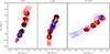 |
Fig. 1 Colourmaps of the sum of the H2 S(0)–S(7) emission (normalized to 1 × 10⁻³ erg cm-2 s-1 sr-1) and contours of the H2O (110−101) emission are overlaid. Red contours are from 0.06 to 19 K km s-1, 0.09 to 55 K km s-1, and 0.05 to 7.9 K km s-1 for L 1157, L 1448, and VLA 1623, respectively. Blue contours for the same sources are from 0.06 to 69 K km s-1, 0.09 to 23 K km s-1, and 0.06 to 10 K km s-1. Offsets in the maps are with respect to the central sources, with coordinates tabulated in Table 1. The black dots indicate the readout positions for the OTF maps. |
2. Observations
The Spitzer observations of the purely rotational H2 transitions, H2 0–0 S(0) to S(7) were originally presented in Neufeld et al. (2009) and we refer the interested reader to that publication.
The mapping observations of the H2O (110−101) emission from the outflows targeted during the WISH program have already been published (Nisini et al. 2013; Bjerkeli et al. 2012) in recent papers, with one exception, viz. L1157. All three maps were obtained with the HIFI instrument using the so-called on-the-fly (OTF) maps with position-switch reference observing mode. The maps cover the 5′ by 2′ regions closest to the central source of the outflows, which means that a large proportion of the L 1448 and L 1157 outflows are covered. In the case of VLA 1623, only a small part of the south-eastern flow is covered by the observations and consequently we exclude this outflow lobe in the analysis. The data were obtained from the Herschel Science Archive (HSA, v8.2.1 of the pipeline) and standard data reduction methods such as baseline removal and production of maps were done in XS and MATLAB. The uncertainty attributed to the calibration is estimated to be ~10% (Roelfsema et al. 2012) and the main beam efficiency at 557 GHz is 0.76 (Olberg 2010). The Herschel observations discussed in the present letter are summarised in Table 1 where the corresponding observation identification numbers are listed.
Observations carried out with HIFI.
Physical parameters derived from CO and H2O observations.
3. Results
For the work presented here, we relied on an estimate of the outflow width and length (when estimating the mass and the dynamical timescale) as measured from the H2O emission, which is why the HPBW of 38′′ at 557 GHz turns out to be a problem. We therefore used a Statistical Image Deconvolution (SID) technique to improve the spatial resolution of the HIFI data (Rydbeck 2008). The deconvolved HIFI maps are presented and overlaid on the Spitzer H2 emission in Fig. 1. From the deconvolution of the maps, we conclude that the widths of the flows are overestimated when using the original datasets. However, the apparent width of the northern flow in L 1157 does not change by a significant amount when the SID method is used, and this part of the flow is likely broader than the southern part. Apart from this single outflow lobe, the outflow lobes have widths of the order ~20′′.
The spatial distributions of the H2 emission regions are in good agreement with the regions responsible for the H2O emission. The most prominent peaks in the H2 emission from all three outflows are coincident with strong H2O peaks. However, we note that the H2O peaks towards the central sources of L 1448 and VLA 1623 are not accompanied by strong H2 peaks. In the original H2O data, we detect a weak red-shifted component in the blue-shifted part of the L 1157 outflow. After deconvolution, this emission stands out and the brightness is significantly enhanced. It will, however, not be discussed further here. Note that the H2O line profiles presented in Nisini et al. (2013) and Bjerkeli et al. (2012) trace velocity ranges equivalent to those of CO. Hence, H2O does not seem to be special insofar as it traces gas moving at higher or lower speeds than CO. The maximum detected velocity for both molecules are in close agreement (i.e. within a few km s-1).
4. Discussion
In this section we compare the physical properties derived from CO observations to those derived from the H2O and H2 observations. Although a resemblance (regarding the spatial distribution and the excitation conditions) between H2O and H2 is well established at this point, it should be noted that this analysis relies on the assumption that the kinematics are also the same. The physical properties of the CO outflows have been presented in André et al. (1990, VLA 1623, Bachiller et al. (1990, L 1448), and Bachiller et al. (2001, L 1157). The results presented in these papers are, however, corrected here using the most recent method for determining these quantities. The question of how outflows are accelerated is still a matter of debate. It has been argued, however, that the highly collimated outflows that are seen to emanate from the very youngest objects (i.e. Class 0 sources) are best explained by jet-driven models (see e.g. Masson & Chernin 1993; Arce et al. 2007). We therefore calculated the dynamical time-scale, momentum, and kinetic energy (td, P, and E respectively) in the same manner suggested by Downes & Cabrit (2007, based on numerical simulations of jet-driven outflows). The inclination angles of the flows with respect to the plane of the sky are assumed to be 21°, 15°, and 9° for L 1448, VLA 1623, and L 1157, respectively (Girart & Acord 2001; Davis et al. 1999; Gueth et al. 1996). It should be noted that uncertainties in the inferred inclination angles do not affect our main conclusions since the introduced errors are equivalent for CO and H2O. The largest relevant contribution to the error budget is instead attributed to the estimated molecular mass M of the outflows. Also, as noted by Downes & Cabrit (2007), to use the intensity-weighted velocity ⟨ υ ⟩ lobe (see e.g. Lada & Fich 1996) averaged over the outflow lobe when determining the dynamical time-scale may overestimate the age of the flow (unless the flow is inclined nearly 90° with respect to the line of sight). Therefore, and as discussed by the same authors, we instead estimate the dynamical ages of the outflows from the maximum velocity, i.e. dividing the extent of the flow with the maximum velocity (corrected for inclinaton) td = Llobe/υmax. The maximum velocity traced by CO is taken from the literature (André et al. 1990; Bachiller et al. 1990, 2001). When estimating the momentum of the flow we use the intensity-weighted velocity and we do not apply any inclination correction. For the kinetic energy we use a correction factor of 5, i.e. the uncorrected value is multiplied by this number (Downes & Cabrit 2007, their Figs. 4 and 5).
The originally published parameters based on CO data are corrected for the most recent distance estimates, 250 pc to L 1157 (Looney et al. 2007), 232 pc to L 1448 (Hirota et al. 2011), and 120 pc to VLA 1623 (Lombardi et al. 2008). The length of the flows are taken to be equal to the maximum extension of the half-power integrated intensity of each lobe. As mentioned earlier, the angular width of all lobes (except the northern flow of L 1157) is close to 20′′. The molecular mass of the H2O emitting regions is calculated from the estimated H2 column density (Nisini et al. 2010b; Giannini et al. 2011; Bjerkeli et al. 2012). We assume the typical velocity of the wind to be 200 km s-1, when estimating the mass-loss rate. All inferred quantities are summarised in Table 2.
The highest detected velocity of the H2O emission line profiles is consistent with previous estimates from CO observations (see Table 2). The dynamical ages of the outflows are of the order 103 years and this confirms that these sources are very young. They may still be in the formation stage where material is accreted onto the proto-stellar condensation. The dynamical age can be compared to the shock propagation time-scale (the time the gas is in a shocked state) for various types of plane-parallel shock models (Bergin et al. 1998; Flower & Pineau des Forêts 2010). For C-type shocks, time-scales are of the order 103 years for a pre-shock density of 104 cm-3, and are even shorter than this for J-type shocks or when pre-shock densities are higher. The dynamical ages can therefore be longer than the time-scales for shock propagation. For the outflows discussed here, the water emitting regions trace gas at densities of ~106 cm-3 and temperatures higher than 100 K. Under these conditions, the time-scale for freeze-out onto grains should be longer than the dynamical time-scale (Bergin et al. 1998; Hollenbach et al. 2009). Thus, it is possible that once the H2O abundance is enhanced due to the presence of a shock it will not be significantly reduced in the post-shock region. This is in agreement with the fact that the H2O emission does not trace gas at particularly high velocities. The thrust dP/dt (momentum rate) and power dE/dt (mechanical luminosity) derived from H2O and H2 are in close agreement with previous estimates based on CO observations. However, although the deviations are small, the thrust is on average three times higher and the power is two times higher when deduced from CO observations (see Fig. 2). The reason for this is not entirely clear, but it may be that the mass of the H2O emitting gas in reality is slightly larger than the values estimated in this work. The wind mass-loss rates are estimated to be ~10-6M⊙ yr-1 for L 1448 and L 1157, and one order of magnitude lower for VLA 1623. Assuming that the luminosity of the central source1 is entirely due to accretion and adopting a radius to mass ratio of 5, this leads to similar values for the mass-accretion rates (see e.g. Stahler et al. 1980).
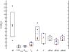 |
Fig. 2 Ratio between parameters inferred from CO and H2O observations. The markers indicate the ratios for L 1448 (squares), VLA 1623 (diamonds), and L 1157 (circles). Red and blue colours are for the red and blue outflow lobes, respectively. Note that a few of the symbols are superpositioned. Dashed lines show the mean and boxes indicate the standard deviation. |
5. Conclusions
The inferred values for power agree to within a factor of 3 when using the different molecular tracers. Similarly, the estimated values for thrust are equal to within a factor of 4. This may indicate that the ejection mechanism that is responsible for the motion of the cold gas, is the same as the one that sets the warm gas into motion. It is, however, also possible that this is a characteristic of young outflows. This study also reveals that the emission from H2O traces a gas component that presumably operates on the same time-scales as CO, i.e. H2O is not detected at very different velocities compared to CO. The fact that the estimated values are the same (within a factor of a few) for all observed sources supports previous estimates based on CO observations. We also find it likely that ground-based CO observations are adequate when assessing the impact of outflows on their environment.
Lbol = 8.3, 8.4, and <2.0 for L 1448, L 1157, and VLA 1623 respectively (Froebrich 2005).
Acknowledgments
P. Bjerkeli wishes to thank Eva Wirström for the interesting discussions. We also appreciate the valuable comments made by the anonymous referee. The authors appreciate the support from the Swedish National Space Board (SNSB). HIFI has been designed and built by a consortium of institutes and university departments from across Europe, Canada, and the United States under the leadership of SRON Netherlands Institute for Space Research, Groningen, The Netherlands, and with major contributions from Germany, France, and the US. Consortium members are: Canada: CSA, U.Waterloo; France: CESR, LAB, LERMA, IRAM; Germany: KOSMA, MPIfR, MPS; Ireland: NUI Maynooth; Italy: ASI, IFSI–INAF, Osservatorio Astrofisico di Arcetri – INAF; The Netherlands: SRON, TUD; Poland: CAMK, CBK; Spain: Observatorio Astronomico Nacional (IGN), Centro de Astrobiologia (CSIC–INTA); Sweden: Chalmers University of Technology – MC2, RSS & GARD; Onsala Space Observatory; Swedish National Space Board, Stockholm University – Stockholm Observatory; Switzerland: ETH Zurich, FHNW; USA: Caltech, JPL, NHSC.
References
- André, P., Martin-Pintado, J., Despois, D., & Montmerle, T. 1990, A&A, 236, 180 [NASA ADS] [Google Scholar]
- André, P., Ward-Thompson, D., & Barsony, M. 1993, ApJ, 406, 122 [NASA ADS] [CrossRef] [Google Scholar]
- Arce, H. G., Shepherd, D., Gueth, F., et al. 2007, in Protostars and Planets V, eds. B. Reipurth, D. Jewitt, & K. Keil, 245 [Google Scholar]
- Bachiller, R., Martin-Pintado, J., Tafalla, M., Cernicharo, J., & Lazareff, B. 1990, A&A, 231, 174 [NASA ADS] [Google Scholar]
- Bachiller, R., Pérez Gutiérrez, M., Kumar, M. S. N., & Tafalla, M. 2001, A&A, 372, 899 [NASA ADS] [CrossRef] [EDP Sciences] [Google Scholar]
- Bergin, E. A., Neufeld, D. A., & Melnick, G. J. 1998, ApJ, 499, 777 [NASA ADS] [CrossRef] [MathSciNet] [Google Scholar]
- Bjerkeli, P., Liseau, R., Larsson, B., et al. 2012, A&A, 546, A29 [NASA ADS] [CrossRef] [EDP Sciences] [Google Scholar]
- Davis, C. J., Smith, M. D., Eislöffel, J., & Davies, J. K. 1999, MNRAS, 308, 539 [NASA ADS] [CrossRef] [Google Scholar]
- de Graauw, T., Helmich, F. P., Phillips, T. G., et al. 2010, A&A, 518, L6 [NASA ADS] [CrossRef] [EDP Sciences] [Google Scholar]
- Downes, T. P., & Cabrit, S. 2007, A&A, 471, 873 [NASA ADS] [CrossRef] [EDP Sciences] [Google Scholar]
- Flower, D. R., & Pineau des Forêts, G. 2010, MNRAS, 406, 1745 [NASA ADS] [Google Scholar]
- Froebrich, D. 2005, ApJS, 156, 169 [NASA ADS] [CrossRef] [Google Scholar]
- Giannini, T., Nisini, B., Neufeld, D., et al. 2011, ApJ, 738, 80 [NASA ADS] [CrossRef] [Google Scholar]
- Girart, J. M., & Acord, J. M. P. 2001, ApJ, 552, L63 [NASA ADS] [CrossRef] [Google Scholar]
- Gueth, F., Guilloteau, S., & Bachiller, R. 1996, A&A, 307, 891 [NASA ADS] [Google Scholar]
- Hirota, T., Honma, M., Imai, H., et al. 2011, PASJ, 63, 1 [NASA ADS] [CrossRef] [Google Scholar]
- Hollenbach, D., Kaufman, M. J., Bergin, E. A., & Melnick, G. J. 2009, ApJ, 690, 1497 [CrossRef] [Google Scholar]
- Kaufman, M. J., & Neufeld, D. A. 1996, ApJ, 456, 611 [NASA ADS] [CrossRef] [Google Scholar]
- Lada, C. J. 1985, ARA&A, 23, 267 [NASA ADS] [CrossRef] [Google Scholar]
- Lada, C. J., & Fich, M. 1996, ApJ, 459, 638 [NASA ADS] [CrossRef] [Google Scholar]
- Lombardi, M., Lada, C. J., & Alves, J. 2008, A&A, 489, 143 [NASA ADS] [CrossRef] [EDP Sciences] [Google Scholar]
- Looney, L. W., Tobin, J. J., & Kwon, W. 2007, ApJ, 670, L131 [NASA ADS] [CrossRef] [Google Scholar]
- Masson, C. R., & Chernin, L. M. 1993, ApJ, 414, 230 [NASA ADS] [CrossRef] [Google Scholar]
- Neufeld, D. A., Nisini, B., Giannini, T., et al. 2009, ApJ, 706, 170 [NASA ADS] [CrossRef] [Google Scholar]
- Nisini, B., Benedettini, M., Codella, C., et al. 2010a, A&A, 518, L120 [NASA ADS] [CrossRef] [EDP Sciences] [Google Scholar]
- Nisini, B., Giannini, T., Neufeld, D. A., et al. 2010b, ApJ, 724, 69 [NASA ADS] [CrossRef] [Google Scholar]
- Nisini, B., Santangelo, G., Antoniucci, S., et al. 2013, A&A, 549, A16 [NASA ADS] [CrossRef] [EDP Sciences] [Google Scholar]
- Olberg, M. 2010, Technical Note: ICC/2010-nnn, v1.1, 2010-11-17 [Google Scholar]
- Pilbratt, G. L., Riedinger, J. R., Passvogel, T., et al. 2010, A&A, 518, L1 [CrossRef] [EDP Sciences] [Google Scholar]
- Poglitsch, A., Waelkens, C., Geis, N., et al. 2010, A&A, 518, L2 [NASA ADS] [CrossRef] [EDP Sciences] [Google Scholar]
- Roelfsema, P. R., Helmich, F. P., Teyssier, D., et al. 2012, A&A, 537, A17 [NASA ADS] [CrossRef] [EDP Sciences] [Google Scholar]
- Rydbeck, G. 2008, ApJ, 675, 1304 [NASA ADS] [CrossRef] [Google Scholar]
- Santangelo, G., Nisini, B., Giannini, T., et al. 2012, A&A, 538, A45 [NASA ADS] [CrossRef] [EDP Sciences] [Google Scholar]
- Stahler, S. W., Shu, F. H., & Taam, R. E. 1980, ApJ, 241, 637 [NASA ADS] [CrossRef] [Google Scholar]
- Tafalla, M., Liseau, R., Nisini, B., et al. 2013, A&A, 551, A116 [NASA ADS] [CrossRef] [EDP Sciences] [Google Scholar]
- Umemoto, T., Iwata, T., Fukui, Y., et al. 1992, ApJ, 392, L83 [NASA ADS] [CrossRef] [Google Scholar]
- van Dishoeck, E. F., Kristensen, L. E., Benz, A. O., et al. 2011, PASP, 123, 138 [NASA ADS] [CrossRef] [Google Scholar]
- Vasta, M., Codella, C., Lorenzani, A., et al. 2012, A&A, 537, A98 [NASA ADS] [CrossRef] [EDP Sciences] [Google Scholar]
- Werner, M. W., Roellig, T. L., Low, F. J., et al. 2004, ApJS, 154, 1 [Google Scholar]
All Tables
All Figures
|
Fig. 1 Colourmaps of the sum of the H2 S(0)–S(7) emission (normalized to 1 × 10⁻³ erg cm-2 s-1 sr-1) and contours of the H2O (110−101) emission are overlaid. Red contours are from 0.06 to 19 K km s-1, 0.09 to 55 K km s-1, and 0.05 to 7.9 K km s-1 for L 1157, L 1448, and VLA 1623, respectively. Blue contours for the same sources are from 0.06 to 69 K km s-1, 0.09 to 23 K km s-1, and 0.06 to 10 K km s-1. Offsets in the maps are with respect to the central sources, with coordinates tabulated in Table 1. The black dots indicate the readout positions for the OTF maps. |
| In the text | |
|
Fig. 2 Ratio between parameters inferred from CO and H2O observations. The markers indicate the ratios for L 1448 (squares), VLA 1623 (diamonds), and L 1157 (circles). Red and blue colours are for the red and blue outflow lobes, respectively. Note that a few of the symbols are superpositioned. Dashed lines show the mean and boxes indicate the standard deviation. |
| In the text | |
Current usage metrics show cumulative count of Article Views (full-text article views including HTML views, PDF and ePub downloads, according to the available data) and Abstracts Views on Vision4Press platform.
Data correspond to usage on the plateform after 2015. The current usage metrics is available 48-96 hours after online publication and is updated daily on week days.
Initial download of the metrics may take a while.