© ESO, 2013

1. Introduction

Tellurium is important in astrophysics and, more particularly, in stellar nucleosynthesis. In 1973 already, Cowley et al. (1973) were able to obtain abundance estimates for 8 elements in the star HR 465 near the r-process peaks at tellurium and osmium. A large overabundance of tellurium was obtained by assuming that the oscillator strengths were equal to log gf = 0.0, which was obviously a rough approximation imposed by the lack of data on oscillator strengths. Recently, neutral tellurium has been detected by Roederer et al. (2012) in three metal-poor stars (BD + 17 3248, HD 108317, and HD 128279) enriched by products of r-process nucleosynthesis using near-ultraviolet spectra obtained with the Space Telescope Imaging Spectrograph on board the Hubble Space Telescope. This element had not been detected previously in Galactic halo stars.

The tellurium ions (Te⁺ and Te²⁺) have not been identified so far in stellar spectra, one of the obvious reasons being the lack of data on oscillator strengths in these two ions, the results available (Biémont et al. 1995) concerning only the forbidden transitions. Another reason results from the fact that a quantitative analysis of Te II lines is complicated by hyperfine structure effects (Werel & Augustyniak 1981). This lack of radiative data justifies the effort of the present work. It is further motivated by the recent new analysis of Te III spectrum carried out by Tauheed & Naz (2011).

2. State-of-the-art analysis of Te II and Te III spectra

The ground configuration of Te II is 5s²5p³. The experimentally known even configurations are 5s5p⁴, 5s²5p²nd (n ≥ 5) and 5s²5p²ns (n ≥ 6). The excited odd ones are of the types 5s²5p²np (n ≥ 6) and 5s²5p²nf (n ≥ 4). The levels compiled in the NIST database (Kramida et al. 2012) are taken from Handrup & Mack (1964) and are characterized by an uncertainty of about 0.2 cm^-1. More accurate level values of the ground configuration (uncertainties in the range 0.004−0.007 cm^-1) are due to Eriksson (1974). The most recent Te II spectrum analysis is due to Tauheed et al. (2009) but the uncertainties are larger (0.4−2.3 cm^-1). The levels considered in the present work have been adopted from the NIST compilation.

Te III belongs to the Sn I isoelectronic sequence and its ground configuration is 5s²5p². The excitation of an outer electron from the ground configuration leads to 5s²5pnd (n ≥ 5) and 5s²5pns (n ≥ 6) while the core excitation gives rise to the 5s5p³ configuration. The first investigations of the Te III spectrum are due to Krishnamurty & Rao (1937) and Joshi & Crooker (1964). More recently, the analysis of the Te III spectrum was revised on the basis of configuration interaction calculations by Joshi et al. (1992) but this work was restricted to transitions connecting the ground configuration and 5s²5p5d, 5s²5p6s and 5s5p³ configurations. The most recent effort in this ion is due to Tauheed & Naz (2011) who investigated the VUV region (30−200 nm). 150 lines were identified and 60 energy levels were established. The present work is essentially based on this analysis.

The prominent lines of Te II emitted from the ground state configuration (5s²5p³) do appear in the short wavelength range between 79 and 184 nm. In Te III, according to Tauheed & Naz (2011), the lines emitted from the ground 5s²5p² configuration are observed in the 50−75 nm wavelength range. However, Joshi et al. (1992) have observed Te III lines between 77−178 nm.

3. Calculations

A traditional way to obtain transition probabilities in a given ion is to combine lifetime measurements (realized e.g. with a laser spectroscopy technique) with branching fractions deduced either from direct measurements in the laboratory or from atomic structure calculations. When the experimental lifetimes are entirely missing, it is necessary to rely on atomic structure calculations. The accuracy of such calculations is difficult to evaluate particularly in the case of heavy ions or atoms. An interesting information on this accuracy is obtained by comparing calculations realized using several different independent theoretical approaches. The agreement (or disagreement) observed when comparing the different sets of results allows to assess the validity of the theoretical models used. This general procedure was followed in the present work.

3.1. MCDHF calculations in Te II and Te III

A first approach used is the multiconfiguration Dirac-Hartree-Fock (MCDHF) method implemented in the GRASP2K computer package (Jonsson et al. 2007). In this method, the atomic state functions (ASFs), Ψ(γJM_J), are expanded in linear combinations of configuration state functions (CSFs), Φ(α_iJM_J), according to: 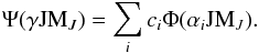$\mathrm{\Psi }\mathrm{\left(}\mathit{\gamma }{\mathrm{JM}}_{\mathit{J}}\mathrm{\right)}\mathrm{=}\sum _{\mathit{i}}{\mathit{c}}_{\mathit{i}}\mathrm{\Phi }\mathrm{\left(}{\mathit{\alpha }}_{\mathit{i}}{\mathrm{JM}}_{\mathit{J}}\mathrm{\right)}\mathit{.}$(1)The CSFs are in turn linear combinations of Slater determinants obtained from monoelectronic spin orbitals of the form: 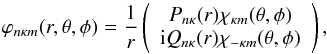${\mathit{\varphi }}_{\mathit{n\kappa m}}\mathrm{\left(}\mathit{r,\theta ,\phi }\mathrm{\right)}\mathrm{=}\frac{\mathrm{1}}{\mathit{r}}\left(\begin{array}{c}\\ {\mathit{P}}_{\mathit{n\kappa }}\mathrm{\left(}\mathit{r}\mathrm{\right)}{\mathit{\chi }}_{\mathit{\kappa m}}\mathrm{\left(}\mathit{\theta ,\phi }\mathrm{\right)}\\ \mathrm{i}{\mathit{Q}}_{\mathit{n\kappa }}\mathrm{\left(}\mathit{r}\mathrm{\right)}{\mathit{\chi }}_{\mathrm{-}\mathit{\kappa m}}\mathrm{\left(}\mathit{\theta ,\phi }\mathrm{\right)}\end{array}\right)\mathit{,}$(2)where P_nκ(r) and Q_nκ(r) are, respectively, the large and the small component of the radial wave functions, and the angular functions χ_κm(θ,φ) are the spinor spherical harmonics (Grant 1988). The α_i represent all the one-electron and intermediate quantum numbers needed to completely define the CSF. γ is usually chosen as the α_i corresponding to the CSFs with the largest weight | c_i | ². The quantum number κ is given by: 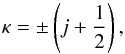$\mathit{\kappa }\mathrm{=}\mathrm{\pm }\left(\mathit{j}\mathrm{+}\frac{\mathrm{1}}{\mathrm{2}}\right)\mathit{,}$(3)where j is the electron total angular momentum. The sign before the parentheses in Eq. (3) corresponds to the coupling relation between the electron orbital momentum, l, and its spin, i.e., $\mathit{l}\mathrm{=}\mathit{j}\mathrm{\pm }\frac{\mathrm{1}}{\mathrm{2}}\mathrm{·}$(4)The radial functions P_nκ(r) and Q_nκ(r) are numerically represented on a logarithmic grid and are required to be orthonormal within each κ symmetry. In the MCDHF variational procedure, the radial functions and the expansion coefficients c_i are optimized to self-consistency.

We have considered the restricted active space (RAS) method for building the MCDHF multiconfiguration expansions. The latter are produced by exciting the electrons from the reference configurations to a given set of orbitals. The rules adopted for generating the configuration space differ according to the correlation model being used. Within a given correlation model, the active set of orbitals spanning the configuration space is increased to monitor the convergence of the total energies and the transition probabilities.

Our calculations have been focused on the E1 transitions 5s²5p^k −(5s5p^k+1 + 5s²5p^k − 1nl) with nl = 5d,6s,6p and k = 3 in Te II and k = 2 in Te III. They have been carried out in six steps for each ion.

In the first step, the core orbitals, i.e. 1s to 4d, together with the 5s and 5p orbitals, have been optimized. All the CSFs (6 in Te II and 5 in Te III) belonging to the ground configuration 5s²5p^k were retained in the configuration space. The energy functional was built within the framework of the average level (AL) option (Grant 1988).

The second step consisted in increasing the configuration space by considering all the CSFs (70 in Te II and 41 in Te III) belonging to the following configurations: 5s²5p^k + 5s5p^k+1 + 5s²5p^k−1{5d,6s,6p}¹. The 5d, 6s, and 6p orbitals have been optimized, keeping the others fixed to their values of the first step. The AL option was chosen to build the energy functional.

In the third step, the configuration space has been extended to, respectively, 12 037 in Te II and 4386 in Te III by considering single and double virtual excitations to the active orbital set {5s,5p,5d,6s,6p,6d} from the multi-reference configurations 5s²5p^k + 5s5p^k+1 + 5s²5p^k−1{5d,6s,6p}¹. Only the 6d orbital has been optimized, fixing all the others to the values of the preceding step using an energy functional built from the lowest 70 ASFs in Te II and the lowest 41 ASFs in Te III within the framework of the extended optimal level (EOL) option (Grant 1988). One can note that, from this step of the computation and onward, core-valence and core-core correlations are also considered through single and double excitations of the 5s core electrons, respectively.

The last three steps consisted in extending further the configuration space by adding to the active set of the preceding steps the following orbitals: 7s, 7p, and 7d in the fourth step giving rise to 37 226 CSFs in Te II and 12 812 CSFs in Te III; 8s, 8p, and 8d in the fifth step generating 76 611 CSFs in Te II and 25 802 CSFs in Te III; and finally, 4f in the last step with 102 359 and 32 724 CSFs generated in Te II and Te III, respectively. In these steps, only the added orbitals have been optimized, the others being fixed using the same energy functional as in the third step; also, single and double virtual electron excitations from the same multi-reference configurations as in the third step have been used to generate the configuration spaces. In Te II, further orbital additions to the active set as well as further opening of the core to include more core-valence and core-core correlations have been prevented by the memory limitations of our computer. We did not attempt to extend further our MCDHF calculation in Te III in order to keep a model equivalent to the one used in Te II.

The comparisons between the experimental (Kramida et al. 2012; Tauheed & Naz 2011) and our MCDHF level energies and Landé factors are shown in Tables 1 and 2 for Te II and Te III, respectively. One can notice that the core-excited levels belonging to 5s5p^k+1 have larger deviations from the experimental energies. This may be explained by the missing core-valence and core-core correlations with the opening of the n ≤ 4 core shells that are implicitly taken into account in our HFR+CPOL calculation through a polarization potential and a fitting procedure (see the next section).

The final MCDHF electric dipole (E1) transition probabilities have been corrected using the experimental energies as follows: 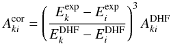${\mathit{A}}_{\mathit{ki}}^{\mathrm{cor}}\mathrm{=}{\left(\frac{{\mathit{E}}_{\mathit{k}}^{\exp }\mathrm{-}{\mathit{E}}_{\mathit{i}}^{\exp }}{{\mathit{E}}_{\mathit{k}}^{\mathrm{DHF}}\mathrm{-}{\mathit{E}}_{\mathit{i}}^{\mathrm{DHF}}}\right)}^{\mathrm{3}}{\mathit{A}}_{\mathit{ki}}^{\mathrm{DHF}}$(5)where ${\mathit{A}}_{\mathit{ki}}^{\mathrm{cor}}$ and ${\mathit{A}}_{\mathit{ki}}^{\mathrm{DHF}}$ are respectively the corrected and MCDHF transition probability of the E1 transition between the upper level k and the lower level i, and ${\mathit{E}}_{\mathit{k}\mathrm{\left(}\mathit{i}\mathrm{\right)}}^{\exp }$ and ${\mathit{E}}_{\mathit{k}\mathrm{\left(}\mathit{i}\mathrm{\right)}}^{\mathrm{DHF}}$ are respectively the experimental and the MCDHF upper (lower) level energy.

These A-values have been determined in the Babushkin and Coulomb gauges, the equivalents of the length and velocity gauges in the non-relativistic limit. A good agreement between these values is a necessary condition for an accurate estimate of the line strength, though it is still not a sufficient condition. We have therefore considered an additional and independent criteria to estimate this accuracy; we have modified the GRASP2K package (Jonsson et al. 2007) to include the calculation of the cancellation factor (CF) as defined by Cowan (1981), i.e.: 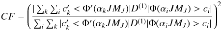$\mathit{CF}\mathrm{=}\left(\frac{\mathrm{|}{\sum }_{\mathit{k}}{\sum }_{\mathit{i}}{\mathit{c}}_{\mathit{k}}^{\mathrm{\prime }}\mathit{<}{\mathrm{\Phi }}^{\mathrm{\prime }}\mathrm{(}{\mathit{\alpha }}_{\mathit{k}}\mathit{J}{\mathit{M}}_{\mathit{J}}\mathrm{\left)}\mathrm{\right|}{\mathit{D}}^{\mathrm{\left(}\mathrm{1}\mathrm{\right)}}\mathrm{\left|}\mathrm{\Phi }\mathrm{\right(}{\mathit{\alpha }}_{\mathit{i}}\mathit{J}{\mathit{M}}_{\mathit{J}}\mathrm{)}\mathit{>}{\mathit{c}}_{\mathit{i}}\mathrm{|}}{{\sum }_{\mathit{i}}{\sum }_{\mathit{k}}\mathrm{|}{\mathit{c}}_{\mathit{k}}^{\mathrm{\prime }}\mathit{<}{\mathrm{\Phi }}^{\mathrm{\prime }}\mathrm{(}{\mathit{\alpha }}_{\mathit{k}}\mathit{J}{\mathit{M}}_{\mathit{J}}\mathrm{\left)}\mathrm{\right|}{\mathit{D}}^{\mathrm{\left(}\mathrm{1}\mathrm{\right)}}\mathrm{\left|}\mathrm{\Phi }\mathrm{\right(}{\mathit{\alpha }}_{\mathit{i}}\mathit{J}{\mathit{M}}_{\mathit{J}}\mathrm{)}\mathit{>}{\mathit{c}}_{\mathit{i}}\mathrm{|}}\right)2$(6)where D⁽¹⁾ is the electric dipole operator and c_i(k)(′) and Φ(′)(α_i(k)JM_J) have the same meanings as in Eq. (1) for the initial (non-primed symbols) and final (primed symbols) states of the transition. A small value of the cancellation factor (say less than 0.05) indicates that the calculated line strength is affected by a strong cancellation effect; this is due to opposite sign contributions of almost equal and significant amplitudes that cancel each other in the transition amplitude expansions which are directly related to the ASF representation (here, in jj coupling). Table 3 illustrates in Te II the complementarity of the gauges agreement criteria and the cancellation factor in the four possible cases, i.e. bad gauges agreement (agreement >10%) and small CF(<0.05), bad gauges agreement and CF > 0.05, good gauges agreement (agreement <10%) and small CF, and good gauges agreement and CF > 0.05; only the last case is indicative of an accurate MCDHF A-value. The corresponding HFR+CPOL transition probabilities and CF values have been also included for comparison.

3.2. Relativistic Hartree-Fock (HFR)

The relativistic Hartree-Fock (HFR) approach including core-polarization (CPOL) effects by means of a model potential and a correction to the transition dipole operator (HFR + CPOL) have been used to investigate the transition probabilities of Te II and Te III.

For Te II, 43 configurations: 5p³ + 5p²6p + 5p²7p + 5p²4f + 5p²5f + 5p²6f + 5d²6p + 5d²6f + 6s²7p + 5d²7p + 4f²5p + 5f²6p + 5s5p³6s + 5s5p³5d + 5s5p³6d + 5s5p²6p5d + 5s5p²6p6d + 5s5p²4f5d + 5s5p²4f6d + 5p⁵ (odd parity) and 5s5p⁴ + 5p²5d + 5p²6d + 5p²7d + 5p²6d + 5p²7d + 5p²6s + 5p²7s + 5p²8s + 5p²5g + 5p²6g + 5d²5g + 5d²6g + 5f²5g + 5f²6g + 5s5p³6p + 5s5p³4f + 5s5p³5f + 5s5p³6f + 5s5p²6s5d + 5s5p²6s6d + 5s5p²5d6d + 5s5p²6s² + 5s5p²5d² (even parity) have been considered.

For Te III, 48 configurations: 5p² + 5p6p + 5p7p + 5p4f + 5p5f + 5p6f + 5d6s + 5d6d + 6s² + 5d² + 4f² + 5f² + 5s5p²6s + 5s5p²5d + 5s5p²6d + 5s5p6s6p + 5s5p6p5d + 5s5p6p6d + 5s5p4f5d + 5s5p4f6d + 5p⁴ + 5p³4f +5p³5f + 5p³6f (even parity) and 5s5p³ + 5p5d + 5p6d + 5p7d + 5p6s + 5p7s + 5p8s + 5p5g + 5p6g + 5d6p + 5d4f + 5d5f + 5d6f + 5s5p²6p + 5s5p²4f + 5s5p²5f + 5s5p²6f + 5s5p6s5d + 5s5p6s6d + 5s5p5d6d + 5s5p6s² + 5s5p5d² + 5p³6s + 5p³5d + 5p³6d (odd parity) were included in the calculations.

In order to consider the CPOL corrections in Te II and Te III calculations, a dipole polarizability of ${\mathit{\alpha }}_{\mathrm{d}}\mathrm{=}\mathrm{1.295}{\mathit{a}}_{\mathrm{0}}^{\mathrm{3}}$ and a cut-off radius of r_c = 0.964  a₀ were adopted. Some radial integrals, considered as free parameters, were then adjusted with a least-squares optimization program minimizing the discrepancies between the calculated Hamiltonian eigenvalues and the experimental energy levels. More precisely, the average energies (E_av), the electrostatic direct (F^k) and exchange (G^k) integrals, the spin-orbit (ζ_nl) and effective interaction (α) parameters were allowed to vary during the fitting process. The scaling factors, i.e. the ratios between the fitted and the HFR values (LSF/HFR), of the optimized parameters ranged between 0.61 to 1.04, 0.50 to 1.19 and 0.85 to 1.19 for, respectively, the F^k, G^k and ζ_nl integrals in Te II. In Te III, these scaling factors became 0.72 ≤ LSF/HFR(F^k) ≤ 0.93, 0.62 ≤ LSF/HFR(G^k) ≤ 0.95 and 0.86 ≤ LSF/HFR(ζ_nl) ≤ 1.27.

For Te II, the energy levels calculated with the HFR+CPOL method are compared to available experimental values in Tables 4 (odd levels) and 5 (even levels), the mean deviations of the fits being found equal to 217 cm^-1 (81 levels, 36 parameters) for the even parity and 87 cm^-1 (45 levels, 19 parameters) for the odd parity. For Te III, the results of the energy levels are included in Tables 6 (even levels) and 7 (odd levels), the mean deviations reaching 100 and 126 cm^-1 for even and odd parity (for the even parity, 14 levels, 9 parameters; for the odd parity, 55 levels, 27 parameters), respectively. The lowest unknown energy levels, i.e. 5s²5p²(¹D)5d ²G_9/2 in Te II and $\mathrm{5}{\mathrm{s}}^{\mathrm{2}}\mathrm{5}\mathrm{p}\mathrm{5}\mathrm{d}{\mathrm{3}}^{}{\mathrm{F}}_{\mathrm{4}}^{\mathrm{o}}$ in Te III, are also given in Tables 5 and 7.

The weighted oscillator strengths (log gf) and transition probabilities (gA) (HFR + CPOL calculations) are reported in Tables 8 (Te II) and 9 (Te III). The electric dipole (E1) transitions between the levels reported in Tables 5−7 with wavelengths less than 1 micrometer and with cancellation factors greater than 0.05 have been selected. In Te II, the list of reported transitions has been further limited to those having a log gf >  − 1. No limit in log gf has been set in Te III. This represents a total number of 439 transitions for Te II and 284 for Te III. Some of these transitions are emitted from high energy levels (>8 eV) and have no chance to be observed in astrophysics. Nevertheless, they are kept in the tables for completion. There are no other (experimental or theoretical) transition probabilities available for comparison.

A majority of the calculated energy levels of Te II obtained with the HFR + CPOL method are strongly mixed, the average LS-purities being equal to 56% and 53% for the odd and even parities, respectively. For Te III, many calculated energy levels are strongly mixed and the average LS-purities of the calculated energy levels obtained by the HFR + CPOL method are equal to 74% and 65% for the even and odd parities, respectively. According to our level LS-compositions in Te III, those given in Tauheed & Naz (2011) should be swapped between the odd levels with J = 2 located at 115 422.2 cm^-1 and at 116 719.4 cm^-1, and between the odd levels with J = 3 located at 120 903.4 cm^-1 and at 127 242.3 cm^-1. Moreover, the first LS-component of the odd levels with J = 3 situated at 120 903.4 cm^-1 is $\mathrm{5}{\mathrm{s}}^{\mathrm{2}}\mathrm{5}\mathrm{p}\mathrm{5}\mathrm{d}{\mathrm{3}}^{}{\mathrm{D}}_{\mathrm{3}}^{\mathrm{o}}$ and not $\mathrm{5}{\mathrm{s}}^{\mathrm{2}}\mathrm{5}\mathrm{p}\mathrm{5}\mathrm{d}{\mathrm{3}}^{}{\mathrm{F}}_{\mathrm{3}}^{\mathrm{o}}$ as this last spectroscopic term appears twice with purities close to 90% in the matrix J = 3 given in the Table 2 of Tauheed & Naz (2011); this was actually a typo as the correct designation was already given in Joshi et al. (1992). Concerning the swapping of designations between the two above-mentioned J = 2 odd levels, although there is an agreement between Tauheed & Naz (2011) and Joshi et al. (1992), our HFR+CPOL designations agree with the NIST database (Kramida et al. 2012) and there is a consistancy with our MCDHF, HFR+CPOL and the experimental Landé g factors (we took the Tauheed & Naz (2011) designations in Table 2 as our MCDHF calculation is in jj-coupling but the experimental Landé g factors follow the NIST database designations which agree with our HFR+CPOL calculation). In addition, it appears that it is actually the ab initio HFR order using both the CI considered in Tauheed & Naz (2011) and our more extended CI expansion.

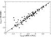Fig. 1 Comparison between MCDHF and HFR+CPOL log gf in Te II. Transitions with CF > 0.05 and gauges agreements better than 10% have been retained. A straight line of equality has been drawn.

Fig. 2 Same as in Fig. 1 for Te III.

4. Discussion

The comparisons between the MCDHF and HFR+CPOL log gf in Te II and Te III are given in Figs. 1 and 2 respectively; only transitions with a gauge agreement better than 10% and CF > 0.05 (in both MCDHF and HFR+CPOL) have been retained. In Te II, the average oscillator strength ratio between HFR+CPOL and MCDHF is 0.99    ±    0.31 (where the second number is the standard deviation) for log gf(HFR+CPOL) ≥ −1 suggesting an accuracy of about 60% (two times the standard deviation) for the strong lines reported in Table 8. Concerning Te III, this ratio becomes 1.21 ± 0.80 due to essentially a few (9 on a total of 65 lines) transitions that present strong disagreements between MCDHF and HFR+CPOL (factor two and more) values. Discarding these lines, we obtain a ratio of 1.07 ± 0.31. For these transitions, the MCDHF transition probabilities prove to have poorly converged; this is illustrated in Fig. 3 where the A-values in both gauges (circles and squares for Babushkin and Coulomb gauges) of one of the problematic transitions ($\mathrm{5}{\mathrm{s}}^{\mathrm{2}}\mathrm{5}{\mathrm{p}}^{\mathrm{2}}{\mathrm{3}}^{}{\mathrm{P}}_{\mathrm{1}}\mathrm{-}\mathrm{5}{\mathrm{s}}^{\mathrm{2}}\mathrm{5}\mathrm{p}\mathrm{6}\mathrm{s}{\mathrm{1}}^{}{\mathrm{P}}_{\mathrm{1}}^{\mathrm{o}}$) along with those of a converged transition ($\mathrm{5}{\mathrm{s}}^{\mathrm{2}}\mathrm{5}{\mathrm{p}}^{\mathrm{2}}{\mathrm{3}}^{}{\mathrm{P}}_{\mathrm{2}}\mathrm{-}\mathrm{5}{\mathrm{s}}^{\mathrm{2}}\mathrm{5}\mathrm{p}\mathrm{6}\mathrm{s}{\mathrm{3}}^{}{\mathrm{P}}_{\mathrm{1}}^{\mathrm{o}}$; diamonds for Babushkin and triangles for Coulomb) are plotted as a function of the calculation step. More correlation orbitals in the active set are clearly needed to stabilize these particular A-values but these calculations were not undertaken in the present work.

5. Conclusions

A first set of transition probabilities has been obtained for 439 transitions of Te II in the spectral range between 77 and 997 nm and for 284 transitions of Te III in the range 52−901 nm. Their accuracy has been assessed through the comparison of the results obtained by two independent theoretical approaches, i.e. the HFR+CPOL and the MCDHF approximations. The satisfying agreement which is observed indicates that the scale of f values is firmly established. This new set of results is expected to help the astrophysicists in the investigation of VUV high resolution spectra and hopefully will contribute to throw some light on nucleosynthesis processes regarding the production of heavy elements in metal-poor stars.

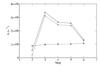Fig. 3 A-values in both gauges (circles and squares for Babushkin and Coulomb gauges) of the $\mathrm{5}{\mathrm{s}}^{\mathrm{2}}\mathrm{5}{\mathrm{p}}^{\mathrm{2}}{\mathrm{3}}^{}{\mathrm{P}}_{\mathrm{1}}\mathrm{-}\mathrm{5}{\mathrm{s}}^{\mathrm{2}}\mathrm{5}\mathrm{p}\mathrm{6}\mathrm{s}{\mathrm{1}}^{}{\mathrm{P}}_{\mathrm{1}}^{\mathrm{o}}$ transition in Te III along with those of $\mathrm{5}{\mathrm{s}}^{\mathrm{2}}\mathrm{5}{\mathrm{p}}^{\mathrm{2}}{\mathrm{3}}^{}{\mathrm{P}}_{\mathrm{2}}\mathrm{-}\mathrm{5}{\mathrm{s}}^{\mathrm{2}}\mathrm{5}\mathrm{p}\mathrm{6}\mathrm{s}{\mathrm{3}}^{}{\mathrm{P}}_{\mathrm{1}}^{\mathrm{o}}$ transition in the same ion (diamonds for Babushkin and triangles for Coulomb) plotted as function of the calculation step. The first transition shows a convergence problem.

Acknowledgments

Financial support from the belgian FRS-FNRS is acknowledged. P.P., P.Q. and E.B. are respectively Research Associate, Research Director and Honorary Research Director of this organization.

References

All Tables

All Figures

	Fig. 1 Comparison between MCDHF and HFR+CPOL log gf in Te II. Transitions with CF > 0.05 and gauges agreements better than 10% have been retained. A straight line of equality has been drawn.
In the text

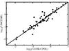	Fig. 2 Same as in Fig. 1 for Te III.
In the text

Fig. 3 A-values in both gauges (circles and squares for Babushkin and Coulomb gauges) of the $\mathrm{5}{\mathrm{s}}^{\mathrm{2}}\mathrm{5}{\mathrm{p}}^{\mathrm{2}}{\mathrm{3}}^{}{\mathrm{P}}_{\mathrm{1}}\mathrm{-}\mathrm{5}{\mathrm{s}}^{\mathrm{2}}\mathrm{5}\mathrm{p}\mathrm{6}\mathrm{s}{\mathrm{1}}^{}{\mathrm{P}}_{\mathrm{1}}^{\mathrm{o}}$ transition in Te III along with those of $\mathrm{5}{\mathrm{s}}^{\mathrm{2}}\mathrm{5}{\mathrm{p}}^{\mathrm{2}}{\mathrm{3}}^{}{\mathrm{P}}_{\mathrm{2}}\mathrm{-}\mathrm{5}{\mathrm{s}}^{\mathrm{2}}\mathrm{5}\mathrm{p}\mathrm{6}\mathrm{s}{\mathrm{3}}^{}{\mathrm{P}}_{\mathrm{1}}^{\mathrm{o}}$ transition in the same ion (diamonds for Babushkin and triangles for Coulomb) plotted as function of the calculation step. The first transition shows a convergence problem.

In the text

References

- Biémont, E., Hansen, J. E., Quinet, P., & Zeippen, C. J. 1995, A&AS, 111, 333 [NASA ADS] [Google Scholar]
- Cowan, R. D. 1981, The Theory of Atomic Structure and Spectra (Berkeley: University of California Press) [Google Scholar]
- Cowley, C. H., Hartoog, M. R., Aller, M. F., & Cowley, A. P. 1973, ApJ, 183, 127 [NASA ADS] [CrossRef] [Google Scholar]
- Crooker, A. M., & Joshi, Y. N. 1964, JOSA, 54 553 [Google Scholar]
- Eriksson, K. B. S. 1974, J. Opt. Soc. Am., 64, 1272 [CrossRef] [Google Scholar]
- Grant, I. P. 1988, in Methods of Computational Chemistry, ed. S. Wilson (New York: Plenum Press), 2, 1 [Google Scholar]
- Handrup, M. B., & Mack, J. E. 1964, Physica (Utrecht), 30, 1245 [NASA ADS] [CrossRef] [Google Scholar]
- Jonsson, P., He, X., Froese Fischer, C., & Grant, I. P. 2007, Comput. Phys. Commun., 177, 597 [NASA ADS] [CrossRef] [MathSciNet] [Google Scholar]
- Joshi, Y. N., Tauheed, A., & Davison, I. G. 1992, Can. J. Phys., 70, 740 [NASA ADS] [CrossRef] [Google Scholar]
- Kramida, A., Ralchenko, Yu., Reader, J., and NIST ASD Team 2012, NIST Atomic Spectra Database (ver. 5.0), available: http://physics.nist.gov/asd, National Institute of Standards and Technology, Gaithersburg, MD [Google Scholar]
- Krishnamurty, S. G., & Rao, K. R. 1937, Proc. R. Soc. London Ser. A, 158, 562 [NASA ADS] [CrossRef] [Google Scholar]
- Roederer, I. U., Lawler, J. E., Cowan, J. J., et al. 2012, ApJ, 747, L8 [Google Scholar]
- Tauheed, A., Joshi, Y. N., & Steinitz, M. 2009, Can. J. Phys., 87, 1255 [NASA ADS] [CrossRef] [Google Scholar]
- Tauheed, A., & Naz, A. 2011, J. Korean Phys. Soc., 59, 2910 [CrossRef] [Google Scholar]
- Werel, K., & Augustyniak, L. 1981, Phys. Scr., 23, 856 [NASA ADS] [CrossRef] [Google Scholar]
All Tables
Comparison between experimental and MCDHF level energies and Landé factors in Te II.
Comparison between experimental and MCDHF level energies and Landé factors in Te III.
Illustration in Te II of the complementarity between the criteria of the gauges agreement and the cancellation factor in the estimation of the A-value accuracy in the four possible cases.
Comparison between experimental and HFR+CPOL level energies and Landé factors in Te II (odd levels).
Comparison between experimental and HFR+CPOL level energies and Landé factors in Te II (even levels).
Comparison between experimental and HFR+CPOL level energies and Landé factors in Te III (even levels).
Comparison between experimental and HFR+CPOL level energies and Landé factors in Te III (odd levels).