| Issue |
A&A
Volume 551, March 2013
|
|
|---|---|---|
| Article Number | L3 | |
| Number of page(s) | 4 | |
| Section | Letters | |
| DOI | https://doi.org/10.1051/0004-6361/201220577 | |
| Published online | 11 February 2013 | |
Turbulent transport in radiative zones of stars
1
CNRS, IRAP,
14 avenue Édouard Belin,
31400
Toulouse,
France
e-mail: This email address is being protected from spambots. You need JavaScript enabled to view it.
2
Université de Toulouse, UPS-OMP, IRAP, Toulouse, France
Received:
16
October
2012
Accepted:
17
January
2013
Abstract
Context. In stellar interiors, rotation is able to drive turbulent motions, and the related transport processes have a significant influence on the evolution of stars. Turbulent mixing in the radiative zones is currently taken into account in stellar evolution models through a set of diffusion coefficients that are generally poorly constrained.
Aims. We want to constrain the form of one of them, the radial diffusion coefficient of chemical elements due to the turbulence driven by radial differential rotation, derived by Zahn (1974, IAU Symp., 59, 185 and 1992, A&A, 265, 115) on phenomenological grounds and largely used since.
Methods. We performed local, direct numerical simulations of stably stratified homogeneous sheared turbulence using the Boussinesq approximation. The domain of low Péclet numbers found in stellar interiors is currently inaccessible to numerical simulations without approximation. It is explored here thanks to a suitable asymptotic form of the Boussinesq equations. The turbulent transport of a passive scalar is determined in statistical steady states.
Results. We provide a first quantitative determination of the turbulent diffusion coefficient and find that the form proposed by Zahn is in good agreement with the results of the numerical simulations.
Key words: diffusion / hydrodynamics / turbulence / stars: interiors / stars: rotation
© ESO, 2013
1. Introduction
As many astrophysical measures are calibrated on stellar evolution theory, realistic stellar evolution models are crucial for astrophysics. One of the major issues is the influence of the macroscopic motions induced by the rotation of a star on its internal structure (see the recent review of Maeder & Meynet 2012). In particular, chemical mixing can significantly extend the lifetime of the stars by continuously providing fresh combustible matter to the core, thus feeding nuclear reactions for a longer time.
A key point of these stellar evolution models is the radial turbulent mixing of chemical
species induced by radial differential rotation. According to Zahn’s model (Zahn 1974), this turbulent mixing is described by a
diffusion coefficient that reads as 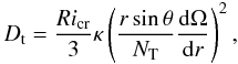 (1)where
κ is the thermal diffusivity,
Ricr the critical value of the Richardson
number, NT the Brunt-Väisälä frequency, and
rsinθdΩ/dr the shear
associated with radial differential rotation. This expression is taken from Eq. (2.14) of
Zahn (1992). While other versions of this diffusion
coefficient exist in the literature, notably those accounting for additional effects like
the μ-gradient (Maeder & Meynet
1996; Talon & Zahn 1997; Mathis et al. 2004), Zahn’s prescription is the basis of
most implementations of the turbulent mixing driven by differential rotation in stellar
evolution codes (Endal & Sofia 1978; Pinsonneault et al. 1989; Heger et al. 2000, see a detailed discussion in Meynet & Maeder 2000). Moreover, this mixing plays a significant role as
compared to other transport processes, such as the meridional circulation combined with
horizontal turbulence, especially for massive stars (Meynet
& Maeder 1997, 2000; Denissenkov et al. 1999) and low-mass stars with strong
μ-gradients (Palacios et al. 2003,
2006). It thus has a direct impact on the
confrontations of stellar evolution models with observations. While chemical abundances at
the star surface have been widely used for such confrontations (Michaud & Zahn 1998; Brott et al.
2011; Potter et al. 2012), asteroseismology
is now providing direct constraints on these processes, especially for subgiant and giant
stars (Deheuvels et al. 2012; Eggenberger et al. 2012).
(1)where
κ is the thermal diffusivity,
Ricr the critical value of the Richardson
number, NT the Brunt-Väisälä frequency, and
rsinθdΩ/dr the shear
associated with radial differential rotation. This expression is taken from Eq. (2.14) of
Zahn (1992). While other versions of this diffusion
coefficient exist in the literature, notably those accounting for additional effects like
the μ-gradient (Maeder & Meynet
1996; Talon & Zahn 1997; Mathis et al. 2004), Zahn’s prescription is the basis of
most implementations of the turbulent mixing driven by differential rotation in stellar
evolution codes (Endal & Sofia 1978; Pinsonneault et al. 1989; Heger et al. 2000, see a detailed discussion in Meynet & Maeder 2000). Moreover, this mixing plays a significant role as
compared to other transport processes, such as the meridional circulation combined with
horizontal turbulence, especially for massive stars (Meynet
& Maeder 1997, 2000; Denissenkov et al. 1999) and low-mass stars with strong
μ-gradients (Palacios et al. 2003,
2006). It thus has a direct impact on the
confrontations of stellar evolution models with observations. While chemical abundances at
the star surface have been widely used for such confrontations (Michaud & Zahn 1998; Brott et al.
2011; Potter et al. 2012), asteroseismology
is now providing direct constraints on these processes, especially for subgiant and giant
stars (Deheuvels et al. 2012; Eggenberger et al. 2012).
The derivation of Zahn’s prescription is based on the hypothesis that turbulent flows are
statistically stationary and that this is achieved when the mean shear flow is close to the
linear marginal stability criterion. Following Townsend
(1958), Zahn modified Richardson’s instability criterion to take the destabilizing
effect of thermal diffusivity into account in such a way that marginal stability is
controlled by RiPe ~ 1, where the Péclet number Pe
compares the diffusive time scale with the dynamical one (as later confirmed through
numerical linear stability analyses, e.g. Lignières et al.
1999). Then, he assumed that, in a turbulent state, the relevant Péclet number in
the expression RiPe ~ 1 is the turbulent one
 , defined
with the turbulent scales of velocity and length (u and ℓ,
respectively). The diffusion coefficient is then estimated through the relation
D = uℓ/3, which finally leads to
Eq. (1).
, defined
with the turbulent scales of velocity and length (u and ℓ,
respectively). The diffusion coefficient is then estimated through the relation
D = uℓ/3, which finally leads to
Eq. (1).
The purpose of our present work is to use local 3D direct numerical simulations (DNS) to test Zahn’s modeling of turbulent mixing. Previous numerical simulations performed in a geophysical context have shown that a steady stably stratified homogeneous sheared turbulence can be obtained by imposing both a uniform mean shear and a uniform stratification and by tuning the Richardson number to reach statistical stationarity (Jacobitz et al. 1997). Such a flow is well adapted to studying chemical turbulent transport and enables one to relate the transport to the local gradients of velocity and entropy as in Zahn’s criterion. Imposing the shear and the stratification amounts to an assumption of scale separation between the variations in the mean and turbulent flows. The main difficulty of performing such numerical simulations in a stellar context is the very low Prandtl number of the stellar fluid. Indeed, this introduces a huge gap between the dynamical time scale and the diffusive one, which forces use of a large number of numerical time steps to accurately compute the effect of thermal diffusion on a dynamical time. This would require a prohibitive amount of computation time for DNS, where the whole range of scales of turbulence down to the dissipative scales are resolved. An attempt to test Zahn’s prescription was made by Brüggen & Hillebrandt (2001), but in this case the simulations relied on the numerical diffusivity of the ZEUS code that is strongly dependent on the grid size (Fromang & Papaloizou 2007). Fortunately, an asymptotic form of the Boussinesq equations in the limit of the small Péclet numbers exists, where the numerical constraint associated with the dynamical effect of the high thermal diffusivity disappears (Lignières 1999).
In this letter, we perform DNS of 3D steady, stably stratified, homogeneous sheared turbulence at decreasing Péclet numbers and use both the Boussinesq equations and the so-called small-Péclet-number approximation (SPNA) to explore the asymptotic Pe ≪ 1 regime. The mathematical model of the considered turbulent flow is presented in Sect. 2, followed by the numerical simulations (Sect. 3) and the methods used to study the turbulent transport (Sect. 4). Then, in Sect. 5, constraints on the diffusion coefficient obtained from our numerical simulations are described and compared to Zahn’s prescription. The results are discussed in Sect. 6.
 |
Fig. 1 Sketch of the flow configuration. |
2. Mathematical model of the flow
To obtain results that are as generic as possible, we consider the simplest flow likely to produce stably stratified, homogeneous, sheared turbulence. Its characteristics are a uniform vertical shear of horizontal velocity and a uniform vertical temperature gradient, as shown in Fig. 1. The governing equations of the flow are presented in Sect. 2.1, and the boundary conditions along with the forcing and the initial conditions in Sect. 2.2.
2.1. Governing equations
We use the Boussinesq equations in which density fluctuations are neglected, except in
the buoyancy term. For the usually low Mach-number flows inside stars, this approximation
is justified as long as the motion vertical length scale is smaller than the pressure
scale height. Using L, ΔU, and
ΔT = (Tmax − Tmin)/2
as length, velocity, and temperature units (see Fig. 1), their non-dimensional form reads as 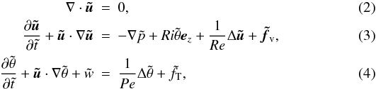 where
where
 is the velocity,
 the pressure deviation from hydrostatic equilibrium,
 the temperature deviation from the mean profile, and
 and
and
 forcing terms (see Sect. 2.2).
These equations show three non-dimensional parameters: (i) the Richardson number Ri = (NT/S)2, noting S = dU/dz = ΔU/L the shear rate, NT2 = αgΔT/L the Brunt-Väisälä frequency, and α the thermal expansion coefficient, (ii) the “macroscopic” Reynolds number Re = LΔU/ν = SL2/ν, where ν is the molecular viscosity, and (iii) the “macroscopic” Péclet number Pe = LΔU/κ = SL2/κ.
To explore the regime of very low Péclet numbers, we use the SPNA (Lignières 1999). The basic principle of this approximation is to
Taylor-expand all variables up to first order in Pe. Thus, Eqs. (3)and (4)become 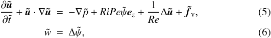 with
with
 . The background thermal
stratification remains fixed because temperature deviations become infinitely small as
Pe approaches zero. There are two non-dimensional parameters left: the
Reynolds number and the “Richardson-Péclet” number RiPe, which compares
the effect of the stratification modified by the thermal diffusion (with a time scale of
τB2/τκ,
where τB = 1/NT
and
τκ = L2/κ
are the buoyancy and diffusive time scales, respectively) to that of the shear. This
number is known to control the linear stability of shear flows at low Péclet number (Lignières et al. 1999, and references herein).
. The background thermal
stratification remains fixed because temperature deviations become infinitely small as
Pe approaches zero. There are two non-dimensional parameters left: the
Reynolds number and the “Richardson-Péclet” number RiPe, which compares
the effect of the stratification modified by the thermal diffusion (with a time scale of
τB2/τκ,
where τB = 1/NT
and
τκ = L2/κ
are the buoyancy and diffusive time scales, respectively) to that of the shear. This
number is known to control the linear stability of shear flows at low Péclet number (Lignières et al. 1999, and references herein).
An expansion similar to the SPNA has been proposed for an unstable thermal stratification (Thual 1992). However, it does not allow the feedback of the convective turbulent motions on the stratification, as observed in the solar convective zone.
The numerical code uses a Fourier colocation method in the horizontal directions, compact finite differences in the vertical, and a projection method plus Runge-Kutta for time advancing.
2.2. Boundary conditions, forcing, and initial conditions
Periodic boundary conditions apply in the horizontal directions, whereas in the vertical
direction the fluid is bounded by two horizontal surfaces that are impenetrable
(w = 0), stress-free in the spanwise direction
(∂zu = 0), uniformly
sheared in the streamwise direction
(∂zv = S),
and thermally controlled (θ = 0). The mean shear profile
U(z) is imposed thanks to a body force
![Mathematical equation: \hbox{$\vec f_{\rm v} = [\vec U(z) - \bar v\vec e_y]/\Delta t$}](/articles/aa/full_html/2013/03/aa20577-12/aa20577-12-eq41.png) applied at every time step Δt, where
applied at every time step Δt, where
 is the horizontal average of the streamwise velocity. The mean vertical temperature
profile is imposed in the same way. With such a set-up, turbulence is not rigorously
homogeneous in the vertical direction. Nevertheless, as already found in Schumacher & Eckhardt (2000) using similar
forcing and boundary conditions, non-homegeneity is limited to thin layers (~10% of the
domain vertical extent) close to the upper and lower boundaries.
is the horizontal average of the streamwise velocity. The mean vertical temperature
profile is imposed in the same way. With such a set-up, turbulence is not rigorously
homogeneous in the vertical direction. Nevertheless, as already found in Schumacher & Eckhardt (2000) using similar
forcing and boundary conditions, non-homegeneity is limited to thin layers (~10% of the
domain vertical extent) close to the upper and lower boundaries.
As initial conditions, we construct a statistically homogeneous and isotropic Gaussian random velocity fluctuation field (Orszag 1969) with an energy spectrum proportional to k2e−k2/k02, where k is the norm of the wave vector and k0 corresponds to the maximum of the spectrum (Jacobitz et al. 1997). The initial temperature deviation θ is set to zero.
3. Numerical simulations
For each value of the Péclet number, the Richardson number can be tuned to obtain statistical steady-state flows. In the regime where thermal diffusivity has no dynamical effect, various studies (Holt et al. 1992; Jacobitz et al. 1997) had already shown there is a critical Richardson number such that the turbulent kinetic energy increases if Ri < Ricr and decreases if Ri > Ricr, as illustrated in Fig. 2. We could also find such critical Richardson numbers in the low-Péclet-number regime.
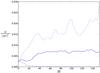 |
Fig. 2 Evolution of the turbulent kinetic energy K for three different Richardson numbers at turbulent Péclet number Peℓ = 52. After a transient regime, the turbulent kinetic energy is stationary for Ri = 0.124, increases for Ri = 0.05 and decreases for Ri = 0.2. |
Moreover, to obtain reliable statistics of the turbulent transport, the simulation domain
must contain several correlation length scales of the turbulence and the duration of the
simulation must be long compared to its correlation time scale. Denoting ℓ
as the horizontal integral length scale defined by
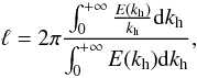 (7)where
E(kh) is the horizontal spectrum of the
turbulent kinetic energy averaged over the vertical direction, we find that the ratio
ℓ/Lh never exceeds 0.16 in
our simulations. This indicates that there are several large structures in the simulated
domain. For illustration, Fig. 3 displays 2D snapshots
of the temperature fluctuations and of the vertical velocity.
(7)where
E(kh) is the horizontal spectrum of the
turbulent kinetic energy averaged over the vertical direction, we find that the ratio
ℓ/Lh never exceeds 0.16 in
our simulations. This indicates that there are several large structures in the simulated
domain. For illustration, Fig. 3 displays 2D snapshots
of the temperature fluctuations and of the vertical velocity.
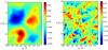 |
Fig. 3 Snapshots of temperature fluctuations scaled by ΔT (left) and vertical velocity scaled by ΔU (right) in the yOz plane at Peℓ = 0.34. Vertical velocity presents smaller scales than temperature fluctuations; both are anti-correlated. |
To properly resolve all scales of turbulence, we use a resolution of 1282 × 257 and an aspect ratio Lh/Lv = π/4. We have verified that in our simulation kmaxη > 1, where kmax is the largest wavevector present in the flow, η = (ν3/ε)1/4 the Kolmogorov dissipation scale, and ε the dissipation rate. This criterion, which states that all scales down to the dissipation scale are resolved, has been found to be adapted for the study of turbulent transport in isotropic turbulence simulations (Gotoh et al. 2002). In addition, simulations performed at a higher resolution have confirmed that our resolution is sufficient.
4. Turbulent transport
The passive scalar is introduced once a statistical steady state is reached. We then consider and compare two complementary approaches to determine its vertical turbulent transport: one Lagrangian, by following fluid particles; the other Eulerian, by solving an advection/diffusion equation for a concentration field.
Owing to the stationarity and the spatial homogeneity of the turbulence, a fluid particle
encounters statistically homegeneous conditions as it moves with the flow (as long as it
keeps away from the upper and lower boundaries). The turbulence is thus homogeneous from a
Lagrangian point of view. This is an important property because it enables us to apply
Taylor’s turbulent transport theory (Taylor 1921).
Accordingly, the transport is diffusive, and the vertical turbulent diffusion coefficient
Dt reads as 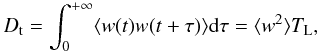 (8)where
TL is the Lagrangian correlation time and ⟨ ⟩ the ensemble
average over the particles. If z(t) denotes the vertical
position of a particle, the vertical dispersion is then given by
(8)where
TL is the Lagrangian correlation time and ⟨ ⟩ the ensemble
average over the particles. If z(t) denotes the vertical
position of a particle, the vertical dispersion is then given by ![Mathematical equation: \begin{equation} \label{eq_D_depl} \left\langle [z(t)-z(0)]^2\right\rangle=2D_{\rm t}t. \end{equation}](/articles/aa/full_html/2013/03/aa20577-12/aa20577-12-eq74.png) (9)We computed the
turbulent diffusivity Dt using either Eq. (8)or a linear regression of the mean square
displacement
(9)We computed the
turbulent diffusivity Dt using either Eq. (8)or a linear regression of the mean square
displacement ![Mathematical equation: \hbox{$\left\langle [z(t)-z(0)]^2\right\rangle$}](/articles/aa/full_html/2013/03/aa20577-12/aa20577-12-eq75.png) . In both
cases the main source of error is the temporal fluctuations of the averaged turbulent
quantities. Then, depending on the starting point of the time average, this creates a
significant dispersion (up to 20%) in the values of Dt. We favor
the turbulent diffusivity Dt obtained with Eq. (8)because in this case the dispersion is
generally lower than using the linear regression of the mean square displacement.
. In both
cases the main source of error is the temporal fluctuations of the averaged turbulent
quantities. Then, depending on the starting point of the time average, this creates a
significant dispersion (up to 20%) in the values of Dt. We favor
the turbulent diffusivity Dt obtained with Eq. (8)because in this case the dispersion is
generally lower than using the linear regression of the mean square displacement.
In the Eulerian approach, the concentration field c is governed by the
equation 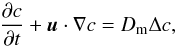 (10)where the molecular
diffusivity Dm is such that
Pec = LΔU/Dm = 104.
To determine Dt, we impose a mean concentration gradient
dC/dz and compute
(10)where the molecular
diffusivity Dm is such that
Pec = LΔU/Dm = 104.
To determine Dt, we impose a mean concentration gradient
dC/dz and compute 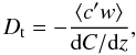 (11)where
c′ refers to the concentration deviation from the mean profile
C(z).
(11)where
c′ refers to the concentration deviation from the mean profile
C(z).
We found that the relative difference between Dt computed from the Lagrangian approach (Eq. (8)) and the Eulerian one does not exceed 15%. This difference is partly due to molecular diffusion, which is present in the Eulerian approach but not in the Lagrangian one. Nevertheless, this effect is limited because Dm/Dt remains always less than 5%. Again, the difference is mostly due to temporal fluctuations of the turbulent quantities that generate dispersion in the time averages. A way to reduce this dispersion is to average over a longer time. While it is not possible in the Lagrangian approach since the displacements of particles are limited by the upper and lower boundaries of the domain, a much longer integration time can be used in the Eulerian one. We have thus used the Eulerian determination of the turbulent diffusion coefficient, keeping the error linked to the time average to a value lower than 5%.
5. Results
We present the results of five simulations corresponding to five different values of the turbulent Péclet number, Peℓ = 52,0.90,0.72,0.34, and ≪ 1 (the last using the SPNA). Table 1 displays the turbulent diffusion coefficients, together with other relevant physical parameters.
Results of the different runs.
The most striking feature is that the full computation at Peℓ = 0.34 and the SPNA computation give similar results. Indeed, at Peℓ = 0.34 the critical Richardson number multiplied by the turbulent Péclet number is very close to the critical “Richardson-Péclet” number of the SPNA computation. This is strong evidence that at small Péclet number, the steady, stably stratified, sheared turbulence is characterized by a critical “Richardson-Péclet” number (RiPeℓ)cr independent of the Péclet number. This regime has not been reached in the simulations from Peℓ = 52 to Peℓ = 0.7 where RicrPeℓ > (RiPeℓ)cr.
Table 1 further shows the parameter
β = Dt/(uℓ),
which in the regime where
RiPeℓ = (RiPeℓ)cr,
verifies 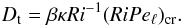 (12)This parameter
clearly has the same value for Pe = 0.34 and Pe ≪ 1. Thus,
in the small-Péclet-number regime, the turbulent diffusion coefficient can be written in the
form of (12)with a constant
β. As a consequence, Dt is proportional to
κRi-1.
(12)This parameter
clearly has the same value for Pe = 0.34 and Pe ≪ 1. Thus,
in the small-Péclet-number regime, the turbulent diffusion coefficient can be written in the
form of (12)with a constant
β. As a consequence, Dt is proportional to
κRi-1.
It is obvious that the final expression found for the vertical turbulent diffusion coefficient Dt (see Eq. (12)) has the same form as Zahn’s prescription given in Eq. (1), thus validating in the Pe ≤ 0.34 range the hypotheses made to derive it. The present numerical simulations also provide a quantitative determination of the critical turbulent “Richardson-Péclet” number (RiPeℓ)cr = 0.426 and of the coefficient β = Dt/(uℓ) ≃ 0.131. This has to be compared with the order of magnitude estimates proposed by Zahn (1992), namely Ric ≲ 1/4 and β = 1/3 ≃ 0.333. Nevertheless, it is the proportionality constant between Dt and κRi-1, i.e. the product of β and (RiPeℓ)cr, which is relevant in practice in stellar evolution codes. We find a value of 5.58 × 10⁻² for this quantity, whereas Zahn’s prescription leads to 8.33 × 10⁻², which is a relative difference of 33%.
6. Conclusion and discussion
We thus conclude that the results of our DNS agree with the form of Zahn’s prescription and provide a first quantitative determination of Dt beyond Zahn’s order of magnitude estimate. In general, the main drawback of numerical simulations of turbulent flows is the unrealistically low value of the Reynolds number. While it may be interesting to test the dependence of our results on the Reynolds number, we note that estimates of effective turbulent Reynolds numbers associated with the radial diffusion of chemicals in stars lead to surprisingly low values Reℓ ~ 100 (Michaud & Zahn 1998), which are comparable to the values obtained in the present work.
Other relevant issues can be addressed numerically. In particular, the concentration field is considered here as a passive scalar so that the mean gradient has no effect on the flow, whereas in reality such a stratification would enhance the effect of temperature stratification. This effect is considered differently by Maeder & Meynet (1996) and Talon & Zahn (1997), and simulations might help in deciding between them. Another important aspect of the models of rotationally-induced mixing is the magnitude of the horizontal turbulent transport driven by the horizontal differential rotation. It controls the efficiency of the meridional circulation transport and the departure from shellular rotation (Zahn 1992). Again, the turbulent transport can be investigated with DNS similar to the present ones by varying the angle between the velocity and temperature gradients.
To study the turbulent transport in less idealized flow configurations would require a better understanding of the shear flows induced by the large-scale motions driven by rotation.
Acknowledgments
This work was granted access to the HPC resources of CALMIP under the allocation 2012–P0507.
References
- Brott, I., Evans, C. J., Hunter, I., et al. 2011, A&A, 530, A116 [NASA ADS] [CrossRef] [EDP Sciences] [Google Scholar]
- Brüggen, M., & Hillebrandt, W. 2001, MNRAS, 320, 73 [NASA ADS] [CrossRef] [Google Scholar]
- Deheuvels, S., Garcia, R. A., Chaplin, W. J., et al. 2012, ApJ, 756, 19 [NASA ADS] [CrossRef] [Google Scholar]
- Denissenkov, P. A., Ivanova, N. S., & Weiss, A. 1999, A&A, 341, 181 [NASA ADS] [Google Scholar]
- Eggenberger, P., Montalbán, J., & Miglio, A. 2012, A&A, 544, L4 [NASA ADS] [CrossRef] [EDP Sciences] [Google Scholar]
- Endal, A. S., & Sofia, S. 1978, ApJ, 220, 279 [NASA ADS] [CrossRef] [Google Scholar]
- Fromang, S., & Papaloizou, J. 2007, A&A, 476, 1113 [NASA ADS] [CrossRef] [EDP Sciences] [Google Scholar]
- Gotoh, T., Fukayama, D., & Nakano, T. 2002, Phys. Fluids, 14, 1065 [NASA ADS] [CrossRef] [MathSciNet] [Google Scholar]
- Heger, A., Langer, N., & Woosley, S. E. 2000, ApJ, 528, 368 [NASA ADS] [CrossRef] [Google Scholar]
- Holt, S. E., Koseff, J. R., & Ferziger, J. H. 1992, J. Fluid Mech., 237, 499 [NASA ADS] [CrossRef] [Google Scholar]
- Jacobitz, F. G., Sarkar, S., & van Atta, C. W. 1997, J. Fluid Mech., 342, 231 [NASA ADS] [CrossRef] [Google Scholar]
- Lignières, F. 1999, A&A, 348, 933 [NASA ADS] [Google Scholar]
- Lignières, F., Califano, F., & Mangeney, A. 1999, A&A, 349, 1027 [NASA ADS] [Google Scholar]
- Maeder, A., & Meynet, G. 1996, A&A, 313, 140 [NASA ADS] [Google Scholar]
- Maeder, A., & Meynet, G. 2012, Rev. Mod. Phys., 84, 25 [NASA ADS] [CrossRef] [Google Scholar]
- Mathis, S., Palacios, A., & Zahn, J.-P. 2004, A&A, 425, 243 [NASA ADS] [CrossRef] [EDP Sciences] [Google Scholar]
- Meynet, G., & Maeder, A. 1997, A&A, 321, 465 [NASA ADS] [Google Scholar]
- Meynet, G., & Maeder, A. 2000, A&A, 361, 101 [NASA ADS] [Google Scholar]
- Michaud, G., & Zahn, J.-P. 1998, Theor. Comput. Fluid Dyn., 11, 183 [Google Scholar]
- Orszag, S. A. 1969, Phys. Fluids, 12, 250 [NASA ADS] [CrossRef] [Google Scholar]
- Palacios, A., Talon, S., Charbonnel, C., & Forestini, M. 2003, A&A, 399, 603 [NASA ADS] [CrossRef] [EDP Sciences] [Google Scholar]
- Palacios, A., Charbonnel, C., Talon, S., & Siess, L. 2006, A&A, 453, 261 [NASA ADS] [CrossRef] [EDP Sciences] [Google Scholar]
- Pinsonneault, M. H., Kawaler, S. D., Sofia, S., & Demarque, P. 1989, ApJ, 338, 424 [NASA ADS] [CrossRef] [Google Scholar]
- Potter, A. T., Tout, C. A., & Brott, I. 2012, MNRAS, 423, 1221 [NASA ADS] [CrossRef] [Google Scholar]
- Schumacher, J., & Eckhardt, B. 2000, Europhys. Lett., 52, 627 [NASA ADS] [CrossRef] [EDP Sciences] [Google Scholar]
- Talon, S., & Zahn, J.-P. 1997, A&A, 317, 749 [Google Scholar]
- Taylor, G. I. 1921, in Proc. London Math. Soc., 196–212 [Google Scholar]
- Thual, O. 1992, J. Fluid Mech., 240, 229 [NASA ADS] [CrossRef] [Google Scholar]
- Townsend, A. A. 1958, J. Fluid Mech., 4, 361 [NASA ADS] [CrossRef] [Google Scholar]
- Zahn, J.-P. 1974, in Stellar Instability and Evolution, eds. P. Ledoux, A. Noels, & A. W. Rodgers, IAU Symp., 59, 185 [Google Scholar]
- Zahn, J.-P. 1992, A&A, 265, 115 [NASA ADS] [Google Scholar]
All Tables
All Figures
|
Fig. 1 Sketch of the flow configuration. |
| In the text | |
|
Fig. 2 Evolution of the turbulent kinetic energy K for three different Richardson numbers at turbulent Péclet number Peℓ = 52. After a transient regime, the turbulent kinetic energy is stationary for Ri = 0.124, increases for Ri = 0.05 and decreases for Ri = 0.2. |
| In the text | |
|
Fig. 3 Snapshots of temperature fluctuations scaled by ΔT (left) and vertical velocity scaled by ΔU (right) in the yOz plane at Peℓ = 0.34. Vertical velocity presents smaller scales than temperature fluctuations; both are anti-correlated. |
| In the text | |
Current usage metrics show cumulative count of Article Views (full-text article views including HTML views, PDF and ePub downloads, according to the available data) and Abstracts Views on Vision4Press platform.
Data correspond to usage on the plateform after 2015. The current usage metrics is available 48-96 hours after online publication and is updated daily on week days.
Initial download of the metrics may take a while.