| Issue |
A&A
Volume 551, March 2013
|
|
|---|---|---|
| Article Number | A86 | |
| Number of page(s) | 11 | |
| Section | The Sun | |
| DOI | https://doi.org/10.1051/0004-6361/201220576 | |
| Published online | 27 February 2013 | |
Effect of partial ionization on wave propagation in solar magnetic flux tubes
1
Solar Physics Group, Departament de Física, Universitat de les
Illes Balears, 07122
Palma de Mallorca,
Spain
e-mail:
This email address is being protected from spambots. You need JavaScript enabled to view it.
2
Instituto de Astrofísica de Canarias, 38200, La Laguna, Tenerife, Spain
3
Departamento de Astrofísica, Universidad de La
Laguna, 38206, La
Laguna, Tenerife,
Spain
4
Centre for Mathematical Plasma Astrophysics, Department of
Mathematics, KU Leuven,
Celestijnenlaan 200B, 3001
Leuven,
Belgium
Received:
16
October
2012
Accepted:
22
January
2013
Abstract
Observations show that waves are ubiquitous in the solar atmosphere and may play an important role for plasma heating. The study of waves in the solar corona is usually based on linear ideal magnetohydrodynamics (MHD) for a fully ionized plasma. However, the plasma in the photosphere and the chromosphere is only partially ionized. Here we theoretically investigate the impact of partial ionization on MHD wave propagation in cylindrical flux tubes in a two-fluid model. We derive the general dispersion relation that takes into account the effects of neutral-ion collisions and the neutral gas pressure. We assumed the neutral-ion collision frequency to be an arbitrary parameter. Specific results for transverse kink modes and slow magnetoacoustic modes are shown. We find that the wave frequencies only depend on the properties of the ionized fluid when the neutral-ion collision frequency is much lower that the wave frequency. For high collision frequencies that realistically represent the solar atmosphere, ions and neutrals behave as a single fluid with an effective density corresponding to the sum of densities of fluids plus an effective sound velocity computed as the average of the sound velocities of ions and neutrals. The MHD wave frequencies are modified accordingly. The neutral gas pressure can be neglected when studying transverse kink waves but it has to be included for a consistent description of slow magnetoacoustic waves. The MHD waves are damped by neutral-ion collisions. The damping is most efficient when the wave frequency and the collision frequency are on the same order of magnitude. For high collision frequencies slow magnetoacoustic waves are more efficiently damped than transverse kink waves. In addition, we find the presence of cut-offs for certain combinations of parameters that cause the waves to become non-propagating.
Key words: Sun: oscillations / Sun: atmosphere / waves / magnetic fields / magnetohydrodynamics (MHD)
© ESO, 2013
1. Introduction
Observations show that magnetohydrodynamic (MHD) waves are ubiquitous in the solar atmosphere. Waves are routinely observed in the corona (e.g.., Tomczyk et al. 2007; Tomczyk & McIntosh 2009; McIntosh et al. 2011), the chromosphere (e.g.., Kukhianidze et al. 2006; De Pontieu et al. 2007; Zaqarashvili et al. 2007; He et al. 2009; Okamoto & De Pontieu 2011), and the photosphere (e.g., Jess et al. 2009; Fujimura & Tsuneta 2009). In addition, waves and oscillations in thin threads of solar prominences have been reported (e.g., Okamoto et al. 2007; Lin et al. 2007, 2009; Ning et al. 2009). These recent observations have motivated a number of theoretical works aiming at understanding the properties of the observed waves using the MHD theory (e.g., Van Doorsselaere et al. 2008; Pascoe et al. 2010, 2012; Terradas et al. 2010; Verth et al. 2010; Soler et al. 2011a,b, 2012a). It is believed that the observed waves may play an important role for the heating of the atmospheric plasma (see, e.g., Erdélyi & Fedun 2007; De Pontieu et al. 2007; McIntosh et al. 2011; Cargill & de Moortel 2011).
The study of waves in the solar corona is usually based on the linear ideal MHD theory for a fully ionized plasma (see Priest 1984; Goedbloed & Poedts 2004). In this context, the paper by Edwin & Roberts (1983) on wave propagation in a magnetic flux tube has been used as a basic reference for subsequent works in this field (see also the papers by, e.g., Wentzel 1979; Cally 1986; Goossens et al. 2009, 2012). The assumption of full ionization is adequate for the coronal plasma. However, the lower temperatures of the chromosphere and the photosphere cause this assumption to become invalid. Therefore, it is necessary to determine the impact of partial ionization on the wave modes discussed in Edwin & Roberts (1983) to perform a realistic theoretical modeling of wave propagation in partially ionized magnetic wave guides.
There are many papers that have studied the effect of neutral-ion collision on MHD waves (see, e.g., Braginskii 1965; De Pontieu et al. 2001; Khodachenko et al. 2004, 2006; Leake et al. 2005; Forteza et al. 2007). Since the present paper deals with wave propagation in a magnetic cylinder, we discuss here those works that studied waves in structured media. In solar plasmas the typical frequency of the observed waves is lower than the expected value of the neutral-ion collision frequency. For this reason the single-fluid theory is usually adopted as a first approximation. The single-fluid approximation assumes a strong coupling between ions and neutrals, so that both fluids behave in practice as a single fluid. Soler et al. (2009a) studied wave propagation in a partially ionized flux tube in the single-fluid approximation. The results of Soler et al. (2009a) show that the waves discussed in Edwin & Roberts (1983) are damped due to neutral-ion collisions. Although partial ionization may be relevant for plasma heating (see Khomenko & Collados 2012), the damping by neutral-ion collisions is in general too weak to explain the observed rapid attenuation. In addition, Soler et al. (2009a) found critical values for the longitudinal wavelength that constrains wave propagation. However, Zaqarashvili et al. (2012) have pointed out that these critical wavelengths may not be physical and may be an artifact of the single-fluid approximation. This is so because the single-fluid approximation misses important effects when short length scales and/or high frequencies are involved. In these cases, the general multifluid description is a more suitable approach (see, e.g., Zaqarashvili et al. 2011). In a multifluid description no restriction is imposed on the relative values of the wave frequency and the neutral-ion collision frequency. In this more general treatment the mathematical complexity of the equations is substantially increased compared to the single-fluid case.
A particular form of the multifluid theory is the two-fluid theory in which ions and electrons are considered together as an ion-electron fluid, i.e., the plasma, while neutrals form another fluid that interacts with the plasma by means of collisions. This approach was followed by Kumar & Roberts (2003), who studied surface wave propagation in a Cartesian magnetic interface. In the study by Kumar & Roberts (2003) the gas pressure of neutrals was neglected, meaning that the dynamics of neutrals was only governed by the friction force with ions. Recently, Soler et al. (2012a) used the two-fluid theory to study resonant Alfvén waves in flux tubes. Soler et al. (2012a) focused on transverse kink waves and, consequently, they also neglected gas pressure.
In the present paper we go beyond these previous studies. We derive the general dispersion relation for waves in cylindrical flux tubes in the two-fluid theory. To do so, we consider a consistent description of the neutral fluid dynamics that includes the effect of neutral gas pressure. This is necessary for a realistic description of magnetoacoustic waves. The use of cylindrical geometry and the consideration of neutral pressure are two significant improvements with respect to the Cartesian model of Kumar & Roberts (2003). The dispersion relation derived here is the two-fluid generalization of the well-known dispersion relation of Edwin & Roberts (1983) for a fully ionized single-fluid plasma. The collision frequency between ions and neutrals and the ionization degree are two important parameters of the model. The impact of these two parameters on the waves discussed by Edwin & Roberts (1983) in the fully ionized case is investigated.
This paper is organized as follows. Section 2 contains a description of the equilibrium configuration and the basic equations. In Sect. 3 we follow a normal mode analysis and derive the general dispersion relation for the wave modes. The case in which neutral gas pressure is neglected is explored in Sect. 4, both analytically and numerically. We compare our results with the previous findings of Kumar & Roberts (2003). Then, we incorporate the effect of neutral gas pressure in Sect. 5. Finally, we discuss the implications of our results and give our main conclusions in Sect. 6.
2. Model and two-fluid equations
We study waves in a partially ionized medium composed of ions, electrons, and neutrals. We use the two-fluid theory in which ions and electrons are considered together as an ion-electron fluid, while neutrals form another fluid that interacts with the ion-electron fluid by means of collisions (see, e.g., Zaqarashvili et al. 2011; Soler et al. 2012a,b; Díaz et al. 2012). Throughout, the subscripts “ie” and “n” refer to ion-electrons and neutrals.
We assume a cylindrically symmetric equilibrium and, for convenience, we use cylindrical
coordinates, namely r, ϕ, and z for the
radial, azimuthal, and longitudinal coordinates. The equilibrium is made of a straight
magnetic flux tube of radius R embedded in an unbounded environment. The
equilibrium magnetic field is straight and constant along the z-direction,
namely B = B ẑ. Gravity is ignored. As a
consequence of the force balance condition, the gradients of the equilibrium gas pressures
of the different species are zero. We also assume a static equilibrium so that there are no
equilibrium flows. We restrict ourselves to the study of linear perturbations superimposed
on the equilibrium state. Hence, the governing equations are linearized (see the general
expressions in, e.g., Zaqarashvili et al. 2011). We
adopt some additional simplifications that enable us to tackle the problem of wave
propagation analytically. We neglect collisions of electrons with neutrals because of the
low momentum of electrons. We also drop from the equations the nonadiabatic mechanisms and
the magnetic diffusion terms since our purpose here is to determine the impact of
neutral-ion collisions only. Thus, the set of coupled differential equations governing
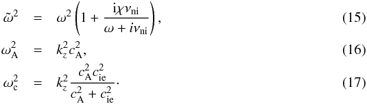
linear perturbations from the equilibrium state are 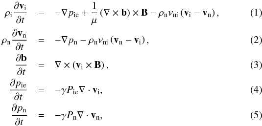 where
vi and vn are the velocities of ions and
neutrals, pie and pn are the
pressure perturbations of ion-electrons and neutrals, b is the magnetic field
perturbation, ρi and ρn are the
equilibrium densities of ions and neutrals, Pie and
Pn are the equilibrium gas pressures of ion-electrons and
neutrals, μ is the magnetic permittivity, γ is the
adiabatic index, and νni is the neutral-ion collision frequency.
For our following analysis it is useful to define the ionization degree as
χ = ρn/ρi.
This parameter ranges from χ = 0 for a fully ionized plasma to
χ → ∞ for a neutral gas. Also for convenience, in the following
expressions we replace the velocities of ions and neutrals by their corresponding Lagrangian
displacements, ξi and
ξn, given by
where
vi and vn are the velocities of ions and
neutrals, pie and pn are the
pressure perturbations of ion-electrons and neutrals, b is the magnetic field
perturbation, ρi and ρn are the
equilibrium densities of ions and neutrals, Pie and
Pn are the equilibrium gas pressures of ion-electrons and
neutrals, μ is the magnetic permittivity, γ is the
adiabatic index, and νni is the neutral-ion collision frequency.
For our following analysis it is useful to define the ionization degree as
χ = ρn/ρi.
This parameter ranges from χ = 0 for a fully ionized plasma to
χ → ∞ for a neutral gas. Also for convenience, in the following
expressions we replace the velocities of ions and neutrals by their corresponding Lagrangian
displacements, ξi and
ξn, given by
 (6)
(6)
3. Normal modes
We assume that the equilibrium densities ρi and
ρn are functions of r alone, so that the
equilibrium is uniform in both azimuthal and longitudinal directions. The temperatures of
ion-electrons and neutrals vary with r accordingly to keep the equilibrium
gas pressures of both fluids constant. Hence we can write the perturbed quantities
proportional to
exp(imϕ + ikzz),
where m and kz are the
azimuthal and longitudinal wavenumbers, respectively. We express the temporal dependence of
the perturbations as exp(−iωt), with ω the frequency.
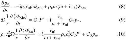
Now we combine Eqs. (1)–(5) and arrive at four coupled equations for the
radial components of the Lagrangian displacements of ions and neutrals,
ξr,ie and
ξr,n, the ion-electron total pressure
Eulerian perturbation,
P′ = pie + Bbz/μ,
and the neutral pressure Eulerian perturbation, pn, namely
 (7)
(7) with
the coefficients
with
the coefficients  ,
,
 ,
,
 ,
and
,
and  defined as
 ![Mathematical equation: \begin{eqnarray} \mathcal{D} &=& \rhoi \left( \va^2 + \csi^2 \right) \left( \omegat^2 - \omegaA^2 \right) \left( \omegat^2 - \omegac^2 \right), \\ \mathcal{C}_1 &=& \frac{m^2}{r^2}\left( \va^2 + \csi^2 \right) \left( \omegat^2 - \omegac^2 \right) \nonumber\\ &&- \left( \omegat^2 - \omegaA^2 \right) \left( \omegat^2 - k_z^2 \csi^2 \right), \\ \mathcal{C}_2 &=&k_z^2 \csi^2 \left( \omegat^2 - \omegaA^2 \right) + \frac{m^2}{r^2}\left( \va^2 + \csi^2 \right) \left( \omegat^2 - \omegac^2 \right) , \\ \mathcal{C}_3 &=& - \left\{ \frac{\nuin^2}{\left( \omega+i\nuin \right)^2} \rhon \csn^2 \left[ \mathcal{C}_2 + \omegaA^2 \left( \omegat^2 - \omegaA^2 \right) \right] \right. \nonumber \\ &&+ \left. \frac{\mathcal{D}}{\omega \left( \omega + i \nuin \right)} \left[ \omega \left( \omega + i \nuin \right)-\csn^2 \left( \frac{m^2}{r^2} + k_z^2 \right)\right] \right\}, \end{eqnarray}](/articles/aa/full_html/2013/03/aa20576-12/aa20576-12-eq42.png) where
where
 ,
,
 , and
, and
 are the squares
of the modified frequency, the Alfvén frequency, and the cusp frequency given by
are the squares
of the modified frequency, the Alfvén frequency, and the cusp frequency given by
 In
addition,
In
addition,  is the square
of the Alfvén velocity and
is the square
of the Alfvén velocity and  and
and
 are the squares
of the sound velocities of ion-electrons and neutrals, respectively, computed as
are the squares
of the sound velocities of ion-electrons and neutrals, respectively, computed as
 (18)Equations (7)–(10) are valid for all density profiles in the radial direction. For
cie = cn = 0 and
pn = 0 they revert to the equations discussed in Soler et al. (2012a). Equations (7)–(10) are singular when
(18)Equations (7)–(10) are valid for all density profiles in the radial direction. For
cie = cn = 0 and
pn = 0 they revert to the equations discussed in Soler et al. (2012a). Equations (7)–(10) are singular when  .
The positions of the singularities are mobile and depend on the frequency,
ω. The whole set of frequencies satisfying
at some r form two continua of frequencies called the Alfvén and cusp (or
slow) continua (see, e.g., Appert et al. 1974). A wave
whose frequency is within any of the two continua is damped by resonant absorption (see,
e.g., Goossens et al. 2011). Resonantly damped waves
in partially ionized magnetic cylinders were studied by Soler et al. (2009b) in the single-fluid approximation and by Soler et al. (2012a) in the two-fluid formalism.
.
The positions of the singularities are mobile and depend on the frequency,
ω. The whole set of frequencies satisfying
at some r form two continua of frequencies called the Alfvén and cusp (or
slow) continua (see, e.g., Appert et al. 1974). A wave
whose frequency is within any of the two continua is damped by resonant absorption (see,
e.g., Goossens et al. 2011). Resonantly damped waves
in partially ionized magnetic cylinders were studied by Soler et al. (2009b) in the single-fluid approximation and by Soler et al. (2012a) in the two-fluid formalism.
3.1. Piece-wise constant equilibrium
In the present paper we are not interested in studying the resonant behavior of the
waves. We refer to Soler et al. (2009b, 2012a) for studies of resonant waves in partially
ionized plasmas. Instead, here we focus on the modification of the wave frequencies due to
neutral-ion collisions. For this reason, we avoid the presence of the resonances by
choosing both ρi and ρn to be
piece-wise constant functions, namely
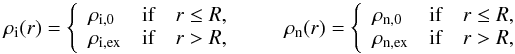 (19)where
R is the radius of the cylinder with constant densities
ρi,0 and
ρn,0 embedded in an external environment
with constant densities ρi,ex and
ρn,ex. This is the density profile adopted
by Edwin & Roberts (1983) in the fully
ionized case. Hereafter the indices “0” and “ex” represent the internal and external
media. Because the magnetic field and equilibrium pressure of both fluids are constant,
the rest of equilibrium quantities are piece-wise constants as well. For simplicity we
also take νni as a constant free parameter.
(19)where
R is the radius of the cylinder with constant densities
ρi,0 and
ρn,0 embedded in an external environment
with constant densities ρi,ex and
ρn,ex. This is the density profile adopted
by Edwin & Roberts (1983) in the fully
ionized case. Hereafter the indices “0” and “ex” represent the internal and external
media. Because the magnetic field and equilibrium pressure of both fluids are constant,
the rest of equilibrium quantities are piece-wise constants as well. For simplicity we
also take νni as a constant free parameter.
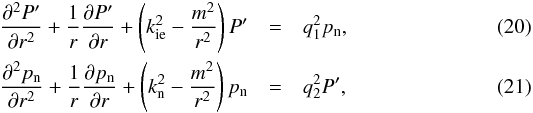
For a piece-wise constant equilibrium we can combine Eqs. (7) and (10) to eliminate
ξr,ie and
ξr,n and obtain two coupled equations
involving P′ and pn only, namely
 with
with
![Mathematical equation: \begin{eqnarray} \ki^2 &=& \frac{\left( \omega \left( \omega + {\rm i} \chi \nuin \right) - \omegaA^2 \right)}{\left( \va^2 + \csi^2 \right)\left( \omegat^2 - \omegac^2 \right)} \nonumber \\ &&\times \left( \omegat^2 - k_z^2 \csi^2 \frac{\omegat^2 - \omegaA^2}{\omega(\omega+{\rm i}\chi\nuin)-\omegaA^2}\right), \\ \kn^2 &=& \frac{\omega \left( \omega + i \nuin \right)-k_z^2 \csn^2 }{\csn^2} \nonumber \\ &&+ \frac{\chi \nuin^2}{\omega + {\rm i} \nuin} \frac{\omega \omegaA^2}{\left( \va^2 + \csi^2 \right)\left( \omegat^2 - \omegac^2 \right)}, \\ q_{\rm 1}^2 &=& {\rm i} \frac{\nuin}{\omega + {\rm i} \nuin} \left[ \frac{\omega \left( \omega + {\rm i} \nuin \right)-k_z^2 \csn^2 }{\csn^2} + \frac{k_z^2 \csi^2 \left( \omegat^2 - \omegaA^2 \right)}{\left( \va^2 + \csi^2 \right)\left( \omegat^2 - \omegac^2 \right)} \right. \nonumber \\ &&+ \left. \frac{\chi \nuin^2}{\omega+{\rm i}\nuin} \frac{\omegaA^2 \omega}{\left( \va^2 + \csi^2 \right)\left( \omegat^2 - \omegac^2 \right)} \right], \\ q_{\rm 2}^2 &=& {\rm i} \frac{\chi \nuin \omega \omegat^2}{\left( \va^2 + \csi^2 \right)\left( \omegat^2 - \omegac^2 \right)}\cdot \end{eqnarray}](/articles/aa/full_html/2013/03/aa20576-12/aa20576-12-eq62.png) Equations
(20) and (21) are the basic equations of this investigation. They are two coupled
Bessel-type differential equations representing the coupled behavior of ion-electrons and
neutrals due to neutral-ion collisions. Note that the terms with
q1 and q2 are the ones that
couple the equations. These terms vanish in fully ionized and fully neutral cases. We need
to solve Eqs. (20) and (21) to find the general dispersion relation.
Equations
(20) and (21) are the basic equations of this investigation. They are two coupled
Bessel-type differential equations representing the coupled behavior of ion-electrons and
neutrals due to neutral-ion collisions. Note that the terms with
q1 and q2 are the ones that
couple the equations. These terms vanish in fully ionized and fully neutral cases. We need
to solve Eqs. (20) and (21) to find the general dispersion relation.
For later use we also give the expressions of
ξr,ie and
ξr,n in terms of
P′ and pn, namely
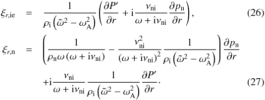 Note
that for νni = 0 ions and neutrals are decoupled and the
magnetic field has no influence on the dynamics of neutrals.
Note
that for νni = 0 ions and neutrals are decoupled and the
magnetic field has no influence on the dynamics of neutrals.
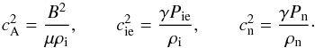
3.2. Strong thermal coupling and characteristic velocities
Up to here, no restriction on the values of the characteristic Alfvén and sound
velocities has been made. As a result of the pressure balance condition at
r = R, the six characteristic velocities in the
equilibrium are related by  (28)Now for simplicity we
assume a strong thermal coupling between the ionized and neutral fluids, so that both
fluids have the same temperature locally. However, the temperature can still be different
in the internal and external media. Using the ideal gas law for both species, this
requirement has the consequence that the local sound velocity of the ionized and neutral
fluids are related by
(28)Now for simplicity we
assume a strong thermal coupling between the ionized and neutral fluids, so that both
fluids have the same temperature locally. However, the temperature can still be different
in the internal and external media. Using the ideal gas law for both species, this
requirement has the consequence that the local sound velocity of the ionized and neutral
fluids are related by  . Hence we
can define an effective sound velocity of the whole plasma,
cs,eff, as
. Hence we
can define an effective sound velocity of the whole plasma,
cs,eff, as 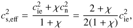 (29)so that the
parameter space of characteristic velocities can be reduced from six to four different
velocities, namely cA,0,
cs,eff,0,
cA,ex, and
cs,eff,ex.
(29)so that the
parameter space of characteristic velocities can be reduced from six to four different
velocities, namely cA,0,
cs,eff,0,
cA,ex, and
cs,eff,ex.
3.3. Coupled solutions
We continue the mathematical study of the normal modes. We look for solutions to the
coupled Eqs. (20) and (21). In the internal medium, i.e.,
r ≤ R, physical solutions imply that both
P′ and pn are regular at
r = 0. The general solutions of P′ and
pn satisfying this condition in the internal medium are
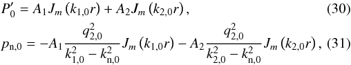 where
Jm is the Bessel function of the first kind
of order m, A1 and
A2 are constants, and
k1,0 and
k2,0 are the two possible values of the
radial wavenumber, k, in the internal medium given by the solution of the
following equation
where
Jm is the Bessel function of the first kind
of order m, A1 and
A2 are constants, and
k1,0 and
k2,0 are the two possible values of the
radial wavenumber, k, in the internal medium given by the solution of the
following equation 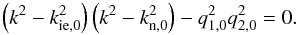 (32)Equivalently, in the
external medium, i.e., r > R,
the solutions of P′ and pn are of
the form
(32)Equivalently, in the
external medium, i.e., r > R,
the solutions of P′ and pn are of
the form 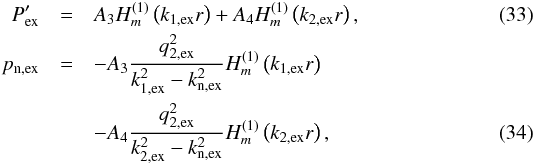 where
where
 is the Hankel function of the first kind of order m,
A3 and A4 are constants, and
k1,ex and
k2,ex are the two possible values of the
radial wavenumber, k, in the external medium also given by the solution
of Eq. (32) but now using external values
for the parameters. The expressions of P′ and
pn for
r > R are written generally in
terms of Hankel functions instead of the usual modified Bessel functions,
Km, used to represent trapped waves. Thus,
our formalism takes into account the possibility of wave leakage, i.e., wave radiation in
the external medium. Although we do not explore leaky waves in the present work, the
obtained dispersion relation will also be valid for leaky waves. For ideal trapped waves,
the external radial wavenumber is purely imaginary and the function
consistently reverts to the modified Bessel function of the second kind,
Km, used by Edwin & Roberts (1983). In the partially ionized case the radial
wavenumber is a complex quantity and the use of the function
causes us to be very careful when choosing the branch of the external radial wavenumber.
To avoid nonphysical energy propagation coming from infinity, we need to select the
appropriate branch of the external radial wavenumber so that the condition for outgoing
waves is satisfied (see details in Cally 1986; Stenuit et al. 1999).
is the Hankel function of the first kind of order m,
A3 and A4 are constants, and
k1,ex and
k2,ex are the two possible values of the
radial wavenumber, k, in the external medium also given by the solution
of Eq. (32) but now using external values
for the parameters. The expressions of P′ and
pn for
r > R are written generally in
terms of Hankel functions instead of the usual modified Bessel functions,
Km, used to represent trapped waves. Thus,
our formalism takes into account the possibility of wave leakage, i.e., wave radiation in
the external medium. Although we do not explore leaky waves in the present work, the
obtained dispersion relation will also be valid for leaky waves. For ideal trapped waves,
the external radial wavenumber is purely imaginary and the function
consistently reverts to the modified Bessel function of the second kind,
Km, used by Edwin & Roberts (1983). In the partially ionized case the radial
wavenumber is a complex quantity and the use of the function
causes us to be very careful when choosing the branch of the external radial wavenumber.
To avoid nonphysical energy propagation coming from infinity, we need to select the
appropriate branch of the external radial wavenumber so that the condition for outgoing
waves is satisfied (see details in Cally 1986; Stenuit et al. 1999).
To understand why there are two different values of the radial wavenumber,
k, it is instructive to assume a weak coupling between the species,
i.e., νni ≪ |ω |, so that the quadratic
terms in νni can be neglected in Eq. (32). The neglected terms involve the coupling
coefficients q1 and q2. Then, the
two independent wavenumbers in Eq. (32)
simplify to 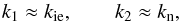 (35)where we have dropped
the indices “0” or “ex” because the same result is valid in both internal and external
media. The two values of k for weak coupling reduce to the wavenumbers of
the ionized and neutral fluids, respectively. For high collision frequencies, these two
wavenumbers contain terms with q1 and
q2 that couple the two fluids.
(35)where we have dropped
the indices “0” or “ex” because the same result is valid in both internal and external
media. The two values of k for weak coupling reduce to the wavenumbers of
the ionized and neutral fluids, respectively. For high collision frequencies, these two
wavenumbers contain terms with q1 and
q2 that couple the two fluids.
3.4. Dispersion relation
To find the dispersion relation we match the internal solutions to the external solutions
by means of appropriate boundary conditions at r = R.
The boundary conditions at the interface between two media in the two-fluid formalism are
discussed in Díaz et al. (2012). In the absence of
gravity, these boundary conditions reduce to the continuity of
P′, pn,
ξr,ie, and
ξr,n at
r = R. After applying the boundary conditions at
r = R we find a system of four algebraic equations for
the constants A1, A2,
A3, and A4. The condition that
the system has a non-trivial solution provides us with the dispersion relation. The
dispersion relation is 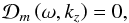 (36)with the full
expression of
(36)with the full
expression of  given in Appendix A. This dispersion relation is
the two-fluid generalization of the dispersion relation of Edwin & Roberts (1983) for a fully ionized single-fluid cylindrical flux
tube. In the following sections we discuss the corrections due to neutral-ion collisions
on the wave modes described by Edwin & Roberts
(1983) in the fully ionized case.
given in Appendix A. This dispersion relation is
the two-fluid generalization of the dispersion relation of Edwin & Roberts (1983) for a fully ionized single-fluid cylindrical flux
tube. In the following sections we discuss the corrections due to neutral-ion collisions
on the wave modes described by Edwin & Roberts
(1983) in the fully ionized case.
4. Pressureless neutral fluid
Before exploring the solutions of the general dispersion relation we first consider the
case that neutral pressure is neglected and only the gas pressure of the ionized fluid is
taken into account. In the absence of neutral pressure the only force acting on the neutral
fluid is the friction force due to neutral-ion collisions. This is the situation studied by
Kumar & Roberts (2003) in planar geometry.
We set Pn = 0 so that cn = 0. After
some algebraic manipulations the general dispersion relation simplifies to 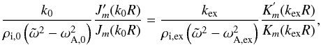 (37)
(37)
with k0 and kex given by
![Mathematical equation: \begin{eqnarray} k_0^2 &=& \frac{\left( \omegat^2 - \omega_{\rm A,0}^2 \right) \left( \omegat^2 - k_z^2 c_{\rm ie,0}^2 \right)}{ \left(c_{\rm A,0}^2 + c_{\rm ie,0}^2\right) \left( \omegat^2 - \omega_{\rm c,0}^2 \right)}\cdot \\[3mm] k_{\rm ex}^2 &=& - \frac{\left( \omegat^2 - \omega_{\rm A,ex}^2 \right) \left( \omegat^2 - k_z^2 c_{\rm ie,ex}^2 \right)}{ \left(c_{\rm A,ex}^2 + c_{\rm ie,ex}^2\right) \left( \omegat^2 - \omega_{\rm c,ex}^2 \right)}\cdot\\[-3mm]\nonumber \end{eqnarray}](/articles/aa/full_html/2013/03/aa20576-12/aa20576-12-eq103.png) In
Eq. (37) we have used the modified Bessel
function of the second kind, Km, instead of the
Hankel function of the first kind, ,
in order to write Eq. (37) in the same form
as the dispersion relation of Edwin & Roberts
(1983). Indeed, the comparison between Eq. (37) and the dispersion relation of Edwin
& Roberts (1983) reveals that both equations are exactly the same if we
replace by
ω2 in Eq. (37). We can take advantage of this result to easily study the modifications due to
neutral-ion collisions of the solutions of the fully ionized case.
In
Eq. (37) we have used the modified Bessel
function of the second kind, Km, instead of the
Hankel function of the first kind, ,
in order to write Eq. (37) in the same form
as the dispersion relation of Edwin & Roberts
(1983). Indeed, the comparison between Eq. (37) and the dispersion relation of Edwin
& Roberts (1983) reveals that both equations are exactly the same if we
replace by
ω2 in Eq. (37). We can take advantage of this result to easily study the modifications due to
neutral-ion collisions of the solutions of the fully ionized case.
4.1. Analytic approximate study
4.1.1. Standing waves
We focus on standing waves so that we fix the longitudinal wavenumber, kz, to a real value. Due to temporal damping by neutral-ion collisions ω is complex. i.e., ω = ωR + iωI, where ωR and ωI are the real and imaginary parts of the frequency. Therefore the wave amplitude is damped in time due through the exponential factor exp(−|ωI|t).
We assume that ω = ω0 is a trapped
solution of the dispersion relation of Edwin &
Roberts (1983) in the fully ionized case. Here we only consider trapped waves
so that ω0 is real. For leaky waves see, e.g., Cally (1986). Then
 is a
solution of Eq. (37). Using the
expression of (Eq.
(15)) we expand the equation
as
is a
solution of Eq. (37). Using the
expression of (Eq.
(15)) we expand the equation
as
 (40)The study of the
modifications due to neutral-ion collisions of the modes of Edwin & Roberts (1983) reduces to the study of the solutions
of Eq. (40). This study is general and
is independent of the particular mode considered since we have not specified what mode
ω0 corresponds to. All modes are affected in the same way
by neutral-ion collisions when neutral pressure is absent.
(40)The study of the
modifications due to neutral-ion collisions of the modes of Edwin & Roberts (1983) reduces to the study of the solutions
of Eq. (40). This study is general and
is independent of the particular mode considered since we have not specified what mode
ω0 corresponds to. All modes are affected in the same way
by neutral-ion collisions when neutral pressure is absent.
Equation (40) is a cubic equation,
hence it has three solutions. To determine the nature of the solutions we perform the
change of variable ω = −is, so that Eq. (40) becomes a cubic equation in
s with all its coefficients real. We compute the discriminant, Δ, of
the resulting equation as ![Mathematical equation: \begin{equation} \Delta= -\omega_0^2 \left[ 4\left(1+\chi \right)^3 \nuin^4 - \left( \chi^2 + 20\chi -8\right)\nuin^2 \omega_0^2 +4 \omega_0^4\right]. \end{equation}](/articles/aa/full_html/2013/03/aa20576-12/aa20576-12-eq116.png) (41)The discriminant, Δ, is
defined so that (i) Eq. (40) has one
purely imaginary zero and two complex zeros when Δ < 0; (ii) Eq.
(40) has a multiple zero and all its
zeros are purely imaginary when Δ = 0; and (iii) Eq. (40) has three distinct purely imaginary zeros when
Δ > 0. This criterion points out that oscillatory solutions of
Eq. (40) are only possible when
Δ < 0.
(41)The discriminant, Δ, is
defined so that (i) Eq. (40) has one
purely imaginary zero and two complex zeros when Δ < 0; (ii) Eq.
(40) has a multiple zero and all its
zeros are purely imaginary when Δ = 0; and (iii) Eq. (40) has three distinct purely imaginary zeros when
Δ > 0. This criterion points out that oscillatory solutions of
Eq. (40) are only possible when
Δ < 0.
To determine when oscillatory solutions are not possible we set Δ = 0 and find the
corresponding relation between ω0 and
νni in terms of χ as ![Mathematical equation: \begin{equation} \frac{\nuin}{\omega_0} = \left[\frac{\chi^2+20\chi-8}{8\left( 1+\chi \right)^3} \pm \frac{\chi^{1/2} \left(\chi-8 \right)^{3/2}}{8\left( 1+\chi \right)^3}\right]^{1/2}\cdot \label{eq:rangenoprop} \end{equation}](/articles/aa/full_html/2013/03/aa20576-12/aa20576-12-eq121.png) (42)\\Since
νni/ω0 must
be real, Eq. (42) imposes a condition on
the minimum value of χ which allows Δ = 0. This minimum value is
χ = 8 and the corresponding critical
νni/ω0 is
(42)\\Since
νni/ω0 must
be real, Eq. (42) imposes a condition on
the minimum value of χ which allows Δ = 0. This minimum value is
χ = 8 and the corresponding critical
νni/ω0 is
 . When
χ < 8 oscillatory solutions are always
possible. When χ > 8 we have to take into
account the + and the − signs in Eq. (42), so that Eq. (42) defines a
range of values of
νni/ω0 in
which oscillatory solutions are not possible. We call this interval the cut-off region.
To our knowledge, Kulsrud & Pearce (1969)
were the first to report on the existence of a cut-off region of MHD waves in a
partially ionized plasma, although Kulsrud &
Pearce (1969) only investigated Alfvén waves in a homogeneous medium. The
existence of cut-off regions for MHD waves in structured media is also deduced from the
plots of Kumar & Roberts (2003), but
these authors did not explore this phenomenon in detail.
. When
χ < 8 oscillatory solutions are always
possible. When χ > 8 we have to take into
account the + and the − signs in Eq. (42), so that Eq. (42) defines a
range of values of
νni/ω0 in
which oscillatory solutions are not possible. We call this interval the cut-off region.
To our knowledge, Kulsrud & Pearce (1969)
were the first to report on the existence of a cut-off region of MHD waves in a
partially ionized plasma, although Kulsrud &
Pearce (1969) only investigated Alfvén waves in a homogeneous medium. The
existence of cut-off regions for MHD waves in structured media is also deduced from the
plots of Kumar & Roberts (2003), but
these authors did not explore this phenomenon in detail.
We look for approximate analytic expressions of the frequency of the oscillatory
solutions. To do this, we assume that
νni/ω0 is
outside the cut-off interval defined by Eq. (42), meaning that Eq. (40) has
two complex (oscillatory) solutions and one purely imaginary (evanescent) solution.
First we focus on the oscillatory solutions. We write
ω = ωR + iωI
and insert this expression into Eq. (40). We assume weak damping and take
| ωI| ≪ |ωR |. Hence we
neglect terms with  and
higher powers. It is crucial for the validity of this approximation that
νni/ω0 is
not within or close to the cut-off region in which ωR = 0.
After some algebraic manipulations we derive approximate expressions for
ωR and ωI. For simplicity we
omit the intermediate steps and give the final expressions, namely
and
higher powers. It is crucial for the validity of this approximation that
νni/ω0 is
not within or close to the cut-off region in which ωR = 0.
After some algebraic manipulations we derive approximate expressions for
ωR and ωI. For simplicity we
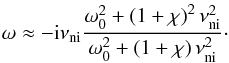
omit the intermediate steps and give the final expressions, namely ![Mathematical equation: \begin{eqnarray} \label{eq:wr} \omega_{\rm R} &\approx & \omega_0 \sqrt{\frac{\omega_0^2+\left( 1 +\chi \right)\nuin^2}{ \omega_0^2+\left( 1 +\chi \right)^2\nuin^2}}, \\[4mm] \label{eq:wi} \omega_{\rm I}&\approx & -\frac{\chi \nuin}{2\left[ \omega_0^2 +\left( 1+\chi \right)^2 \nuin^2\right]} \omega_0^2. \end{eqnarray}](/articles/aa/full_html/2013/03/aa20576-12/aa20576-12-eq133.png) A
mode with the same ωI but with
ωR of opposite sign is also a solution. When
νni = 0, so that neutral-ion collisions are absent, we
find ωR = ω0 and
ωI = 0. Hence we recover the ideal undamped modes of Edwin & Roberts (1983). Now these modes are
damped due to neutral-ion collisions and the frequency has an imaginary part. In
addition, the real part of the frequency is also modified.
A
mode with the same ωI but with
ωR of opposite sign is also a solution. When
νni = 0, so that neutral-ion collisions are absent, we
find ωR = ω0 and
ωI = 0. Hence we recover the ideal undamped modes of Edwin & Roberts (1983). Now these modes are
damped due to neutral-ion collisions and the frequency has an imaginary part. In
addition, the real part of the frequency is also modified.
It is instructive to study the limit values of νni. For a
low collision frequency,  . Equations
(43) and (44) become
. Equations
(43) and (44) become ![Mathematical equation: \begin{eqnarray} \label{eq:wrll} \omega_{\rm R} &\approx & \omega_0, \\[2mm] \label{eq:will} \omega_{\rm I}&\approx & -\frac{\chi \nuin}{2}\cdot \end{eqnarray}](/articles/aa/full_html/2013/03/aa20576-12/aa20576-12-eq138.png) Thus,
the real part of the frequency when is just the
frequency found in the fully ionized case (Edwin
& Roberts 1983) and it does not depend on the amount of neutrals. The
imaginary part of the frequency is independent of ω0,
meaning that it is the same for all wave modes. On the other hand, for a high collision
frequency,
Thus,
the real part of the frequency when is just the
frequency found in the fully ionized case (Edwin
& Roberts 1983) and it does not depend on the amount of neutrals. The
imaginary part of the frequency is independent of ω0,
meaning that it is the same for all wave modes. On the other hand, for a high collision
frequency,  and Eqs.
(43) and (44) simplify to
and Eqs.
(43) and (44) simplify to ![Mathematical equation: \begin{eqnarray} \label{eq:wrgg}\omega_{\rm R} &\approx & \frac{\omega_0}{\sqrt{1+\chi}}, \\[4mm] \label{eq:wigg}\omega_{\rm I}&\approx & -\frac{\chi \omega_0^2}{2\left( 1+\chi \right)^2 \nuin} \cdot \end{eqnarray}](/articles/aa/full_html/2013/03/aa20576-12/aa20576-12-eq140.png) Now
the expression of ωR involves χ in the
denominator, so that the larger the amount of neutrals, the lower
ωR compared to the frequency in the fully ionized case.
The frequency is reduced by the factor
Now
the expression of ωR involves χ in the
denominator, so that the larger the amount of neutrals, the lower
ωR compared to the frequency in the fully ionized case.
The frequency is reduced by the factor  compared to the fully ionized value. This is the same factor as found by Kumar & Roberts (2003) and is equivalent to
replace the ion density by the sum of densities of ions and neutrals or, equivalently,
to replace ρi by
(1 + χ)ρi. The imaginary part of the
frequency depends now on ω0, meaning that the various modes
have different damping rates.
compared to the fully ionized value. This is the same factor as found by Kumar & Roberts (2003) and is equivalent to
replace the ion density by the sum of densities of ions and neutrals or, equivalently,
to replace ρi by
(1 + χ)ρi. The imaginary part of the
frequency depends now on ω0, meaning that the various modes
have different damping rates.
In addition to the oscillatory solutions, Eq. (40) has one purely imaginary solution whose approximation is given by
 (49)\\The perturbations
related to these modes are evanescent in time. There exists a different evanescent
solution related to each mode, ω0, of the fully ionized
case. Purely imaginary solutions were also found by Zaqarashvili et al. (2011), who studied waves in a partially ionized
homogeneous medium. These modes are not present in the fully ionized case. These
evanescent perturbations may be relevant during the excitation of the waves, since part
of the energy used to excite the waves may go to these modes instead of being used to
excite the oscillatory solutions. This could be investigated by going beyond the present
normal mode analysis and solving the initial value problem.
(49)\\The perturbations
related to these modes are evanescent in time. There exists a different evanescent
solution related to each mode, ω0, of the fully ionized
case. Purely imaginary solutions were also found by Zaqarashvili et al. (2011), who studied waves in a partially ionized
homogeneous medium. These modes are not present in the fully ionized case. These
evanescent perturbations may be relevant during the excitation of the waves, since part
of the energy used to excite the waves may go to these modes instead of being used to
excite the oscillatory solutions. This could be investigated by going beyond the present
normal mode analysis and solving the initial value problem.
4.1.2. Propagating waves
Now we turn to propagating waves. In the fully ionized case the study of propagating waves is equivalent to that of standing waves. Here we shall see that neutral-ion collisions break this equivalence and propagating waves are worth being studied separately. Propagating waves were not investigated by Kumar & Roberts (2003). For propagating waves, we fix the frequency, ω, to a real value and solve the dispersion relation for the complex kz, i.e., kz = kz,R + ikz,I, where kR and kI are the real and imaginary parts of kz. Therefore the wave amplitude is damped in space due to the exponential factor exp(−kz,Iz).
Equation (37) also holds for
propagating waves. We assume that
kz = kz,0,
with kz,0 real, is a solution of the ideal
dispersion relation of Edwin & Roberts
(1983). Then, 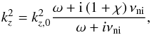 (50)\\is a solution of Eq.
(37) following the same argument as
explained for standing waves. We write
kz = kz,R + ikz,I
and insert this expression in Eq. (50).
We obtain exact expressions for kz,R and
kz,I, namely
(50)\\is a solution of Eq.
(37) following the same argument as
explained for standing waves. We write
kz = kz,R + ikz,I
and insert this expression in Eq. (50).
We obtain exact expressions for kz,R and
kz,I, namely ![Mathematical equation: \begin{eqnarray} k_{z,\rm R} &=& k_{z,0} \sqrt{\frac{\omega^2+(1+\chi)\nuin^2}{2\left( \omega^2+\nuin^2 \right)}} \nonumber \\ &&\times \left[ 1 \pm \left( 1 + \frac{\chi^2\nuin^2\omega^2}{\left( \omega^2+(1+\chi)\nuin^2 \right)^2} \right)^{1/2} \right]^{1/2}, \label{eq:ksr2} \\ k_{z,\rm I} &=& \frac{k_{z,0}^2}{2k_{z,\rm R}} \frac{\chi\nuin\omega}{\omega^2+\nuin^2}\cdot \end{eqnarray}](/articles/aa/full_html/2013/03/aa20576-12/aa20576-12-eq153.png) The
same values of kz,R and
kz,I but with opposite signs are also
solutions. In principle, Eq. (51) allows
two different values of kz,R because of the
± sign. However, the solution with the − sign is not physical since it corresponds to
kz,R imaginary, which is an obvious
contradiction. For this reason we discard the solution with the − sign and take the +
sign in Eq. (51). Now we realize that
The
same values of kz,R and
kz,I but with opposite signs are also
solutions. In principle, Eq. (51) allows
two different values of kz,R because of the
± sign. However, the solution with the − sign is not physical since it corresponds to
kz,R imaginary, which is an obvious
contradiction. For this reason we discard the solution with the − sign and take the +
sign in Eq. (51). Now we realize that
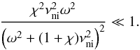 (53)Thus we can
approximate kz,R and
kz,I as
(53)Thus we can
approximate kz,R and
kz,I as  These
expressions are equivalent to Eqs. (43)
and (44) obtained for standing waves.
However, contrary to Eqs. (43) and
(44), Eqs. (54) and (55) are valid for all values of the ratio
νni/ω. There is no
cut-off region for propagating waves because
kz,R never vanishes. There are no purely
imaginary solutions of kz, i.e., all the
solutions always have an oscillatory behavior in z. This is an
important difference to standing waves.
These
expressions are equivalent to Eqs. (43)
and (44) obtained for standing waves.
However, contrary to Eqs. (43) and
(44), Eqs. (54) and (55) are valid for all values of the ratio
νni/ω. There is no
cut-off region for propagating waves because
kz,R never vanishes. There are no purely
imaginary solutions of kz, i.e., all the
solutions always have an oscillatory behavior in z. This is an
important difference to standing waves.
4.2. Comparison with numerical results
Here we numerically solve the dispersion relation (Eq. (37)). For simplicity we focus on standing waves and show the results
for transverse kink (m = 1) waves only, although we have checked that
equivalent results are found for other modes as, e.g., slow magnetoacoustic modes. In the
fully ionized case, the frequency of the transverse kink waves in the thin tube (TT)
limit, i.e., kzR ≪ 1, is
ω = ωk, with ωk
the kink frequency given by  (56)Figure 1 displays the real and imaginary parts of the frequency
of the kink mode as functions of the ratio
νni/ωk for a
particular choice of parameters given in the caption of the figure. We compare the
numerical results with the analytic approximations. In Fig. 1 we have considered χ < 8 so that no
cut-off region is present. Regarding the real part of the frequency (Fig. 1a), we obtain that for
νni/ωk ≪ 1
the results are independent of the ionization degree, with
ωR ≈ ωk as in the fully ionized
case. When the ratio
νni/ωk
increases, plasma and neutrals are more coupled and the ionization degree becomes a
relevant parameter, so that ωR decreases until de value
(56)Figure 1 displays the real and imaginary parts of the frequency
of the kink mode as functions of the ratio
νni/ωk for a
particular choice of parameters given in the caption of the figure. We compare the
numerical results with the analytic approximations. In Fig. 1 we have considered χ < 8 so that no
cut-off region is present. Regarding the real part of the frequency (Fig. 1a), we obtain that for
νni/ωk ≪ 1
the results are independent of the ionization degree, with
ωR ≈ ωk as in the fully ionized
case. When the ratio
νni/ωk
increases, plasma and neutrals are more coupled and the ionization degree becomes a
relevant parameter, so that ωR decreases until de value
 is reached. This behavior is consistent with the analytic Eq. (43) although the details of the transition are
not fully captured by the approximation. Regarding the imaginary part of the frequency
(Fig. 1b), we find that
ωI tends to zero in the limits
νni/ωk ≪ 1
and νni/ωk ≫ 1.
The damping is most efficient when νni and
ωk are, approximately, on the same order of magnitude. This
result is also consistent with the analytic Eq. (44), although the approximation underestimates the actual damping rate when
ωI is minimal. This is so because Eq. (44) was derived in the weak damping
approximation, i.e.,
| ωI| ≪ |ωR |, while
| ωI | and | ωR | are on the
same order when ωI is minimal, meaning that the damping is
strong.
is reached. This behavior is consistent with the analytic Eq. (43) although the details of the transition are
not fully captured by the approximation. Regarding the imaginary part of the frequency
(Fig. 1b), we find that
ωI tends to zero in the limits
νni/ωk ≪ 1
and νni/ωk ≫ 1.
The damping is most efficient when νni and
ωk are, approximately, on the same order of magnitude. This
result is also consistent with the analytic Eq. (44), although the approximation underestimates the actual damping rate when
ωI is minimal. This is so because Eq. (44) was derived in the weak damping
approximation, i.e.,
| ωI| ≪ |ωR |, while
| ωI | and | ωR | are on the
same order when ωI is minimal, meaning that the damping is
strong.
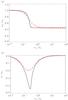 |
Fig. 1 a)ωR/ωk and b) ωI/ωk versus νni/ωk for the transverse kink (m = 1) mode with kzR = 0.1, ρi,0/ρi,ex = 3, cie,0/cA,0 = 0.2, and χ = 4. The solid line is the result obtained by numerically solving the dispersion relation in the absence of neutral pressure (Eq. (37)). The symbols are the approximate analytic results in the weak damping approximation (Eqs. (43) and (44)). |
Now we take χ > 8 and repeat the previous computations. The results are shown in Fig. 2. We notice the presence of a cut-off region for a certain range of νni/ωk. In this cut-off region ωR = 0. The location of the cut-off region agrees very well with the range given by Eq. (42). This zone exists for relatively low νni/ωk. In the solar atmosphere the expected value of the collision frequency (see, e.g., De Pontieu et al. 2001, Figs. 1 and 2) is much higher than the frequency of the observed waves (e.g., De Pontieu et al. 2007; Okamoto & De Pontieu 2011). The minimum value of the neutral-ion collision frequency in the solar atmosphere is on the order of 10 Hz, while the dominant frequency in the observations of chromospheric kink waves by Okamoto & De Pontieu (2011) is around 22 mHz. Therefore, the cut-off region found here is not in the range of νni/ωk consistent with solar atmospheric parameters and observed wave frequencies. However, in other astrophysical situations the presence of the cut-off region may be relevant (see Kulsrud & Pearce 1969). As expected, the analytic approximations (Eqs. (43) and (44)) completely miss the presence of the cut-off region, although they are reasonably good far from the location of the cut-off.
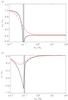 |
Fig. 2 Same as Fig. 1 but with χ = 20. The shaded area denotes the cut-off region given by Eq. (42). |
It is worth mentioning again that the effect of resonant absorption on the damping of transverse kink waves is absent because we used a piece-wise constant density profile (Ruderman & Roberts 2002; Goossens et al. 2002). Soler et al. (2012a) showed that damping by resonant absorption is more efficient than damping by neutral-ion collisions when νni/ωk ≫ 1. Hence, the actual damping of transverse kink waves would be stronger than the damping shown here if resonant absorption were taken into account (see details in Soler et al. 2012a).
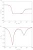 |
Fig. 3 a)ωR/ωc,0 and b) ωI/ωc,0 versus νni/ωc,0 for the slow magnetoacoustic mode with χ = 4 and the rest of parameters the same as in Fig. 1. The solid line is the full result taking neutral pressure into account, while the dashed line is the result when neutral pressure is absent. |
5. Role of neutral pressure
We incorporate the effect of neutral pressure. We anticipate that neutral pressure is
relevant for slow magnetoacoustic waves, while its effect on transverse kink waves is minor.
Goossens et al. (2009, 2012) showed that transverse kink waves in flux tubes have the typical
properties of surface Alfvén (or Alfvénic) waves. In thin tubes, i.e.,
kzR ≪ 1, the main
restoring force of these waves is magnetic tension and the gas pressure force is negligible.
We computed the kink mode frequency in the presence of neutral pressure and found no
significant differences with the result in the absence of neutral pressure. Hence, here we
focus on the study of slow magnetoacoustic waves and explore the modification of the slow
mode frequency due to neutral-ion collisions when neutral pressure is taken into account. In
the fully ionized case (Edwin & Roberts 1983),
slow magnetoacoustic waves in the TT limit have frequencies
ω ≈ ωc,0, with
ωc,0 the internal cusp frequency given by
 (57)This result is independent
of the azimuthal wavenumber, m. In a low-β plasma, i.e.,
when the magnetic pressure is much more important than the gas pressure,
ωc,0 ≈ kzcie,0.
Due to the complexity of the general dispersion relation (Eq. (36)) it is not possible to obtain simple analytic approximations of the
slow mode frequency. For this reason we perform this investigation in a numerical way.
(57)This result is independent
of the azimuthal wavenumber, m. In a low-β plasma, i.e.,
when the magnetic pressure is much more important than the gas pressure,
ωc,0 ≈ kzcie,0.
Due to the complexity of the general dispersion relation (Eq. (36)) it is not possible to obtain simple analytic approximations of the
slow mode frequency. For this reason we perform this investigation in a numerical way.
Figure 3 shows the numerically obtained real and
imaginary parts of the slow mode frequency as functions of the ratio
νni/ωc,0
for χ < 8. The rest of parameters are given in the
caption of the figure. For comparison, we overplot the results in the absence of neutral
pressure, which are obtained by solving Eq. (37) with the same parameters. First we discuss the behavior of the
ωR (Fig. 3a). When
νni/ωc,0 ≪ 1
we recover the result in the fully ionized case, i.e.,
ωR ≈ ωc,0. When
νni/ωc,0
increases, the real part of the slow mode frequency decreases until a plateau is reached at
the value  .
This is equivalent to performing the replacements
.
This is equivalent to performing the replacements  and
and
 in Eq.
(57) and is the same behavior as that
found in the absence of neutral pressure, so that both results are superimposed in Fig.
3a. However, as the ratio
νni/ωc,0
continues to increase, the real part of the frequency rises again until a second plateau is
finally reached. The presence of this second plateau of ωR for
high collision frequencies owes its existence to the effect of neutral pressure and is
absent when neutral pressure is neglected.
in Eq.
(57) and is the same behavior as that
found in the absence of neutral pressure, so that both results are superimposed in Fig.
3a. However, as the ratio
νni/ωc,0
continues to increase, the real part of the frequency rises again until a second plateau is
finally reached. The presence of this second plateau of ωR for
high collision frequencies owes its existence to the effect of neutral pressure and is
absent when neutral pressure is neglected.
We now analyze in detail the second plateau of ωR at high
collision frequencies. Since we have no simple analytic expressions for the slow-mode
frequency we performed a parameter study. We considered various values of
cie and numerically computed the slow mode
ωR at the second plateau. The result of this parameter study
(not shown here for simplicity) points out that the value of ωR
at the second plateau is, approximately,  (58)This expression can
be obtained from Eq. (57) by performing the
replacements and
(58)This expression can
be obtained from Eq. (57) by performing the
replacements and
 , with the
expression of the effective sound velocity,
cs,eff, given in Eq. (29). In a low-β plasma,
, with the
expression of the effective sound velocity,
cs,eff, given in Eq. (29). In a low-β plasma,
 and
ωc,0 ≈ kzcie,0
so that Eq. (58) simplifies to
and
ωc,0 ≈ kzcie,0
so that Eq. (58) simplifies to
 (59)Hence, for practical
purposes we obtain that at high collision frequencies the sound velocity of the ionized
fluid has to be replaced by the effective sound velocity in the expressions of the
frequency. The effective sound velocity takes into account the sound velocity of neutrals in
addition to the sound velocity of ions. In contrast, for intermediate collision frequencies
it is enough to replace cie by
(59)Hence, for practical
purposes we obtain that at high collision frequencies the sound velocity of the ionized
fluid has to be replaced by the effective sound velocity in the expressions of the
frequency. The effective sound velocity takes into account the sound velocity of neutrals in
addition to the sound velocity of ions. In contrast, for intermediate collision frequencies
it is enough to replace cie by
 ,
so that the sound velocity of neutrals can be ignored.
,
so that the sound velocity of neutrals can be ignored.
We turn to the imaginary part of the frequency (Fig. 3b). As for the real part of the frequency, there are striking differences between the results with and without neutral pressure. The full result shows the presence of two different minima of ωI, whereas only the first minimum is present in the absence of neutral pressure. The second minimum takes place in the range of high collision frequencies compared to the ideal cusp frequency. As a consequence of the presence of this second minimum for high collision frequencies, the efficiency of neutral-ion collisions for the damping of the slow mode is higher than for transverse kink modes when νni approaches realistic values. The stronger damping of the slow modes due to neutral-ion collisions compared to the weak damping of the transverse kink modes was already obtained by Soler et al. (2009a) in the single-fluid approximation.
Now we consider χ > 8 and repeat the previous computations (see Fig. 4 for χ = 20). As in the case without neutral pressure, we notice the presence of a cut-off region that agrees well with the range given by Eq. (42). The existence of the cut-off region is not affected by neutral pressure, i.e., the location of the cut-off region is the same as when neutral pressure is neglected. For the set of parameters considered in Fig. 4 the cut-off region appears in the vicinity of νni/ωc,0 ≈ 10-1. We increase the ionization fraction to χ = 100 (Fig. 5). In addition to the cut-off region described above, now we find a second cut-off region. The second cut-off region appears for relatively high collision frequencies, νni/ωc,0 ≈ 101 for the set of parameters used in Fig. 5. This new cut-off region is only present when neutral pressure is taken into account. The result in the absence of neutral pressure completely misses this second cut-off region. The existence of a second cut-off region is a result of slow modes only, since it is not found for transverse kink modes. Unfortunately, unlike for the first cut-off region, we have no analytic expression that gives us the location of the second cut-off region. Instead, out numerical study informs us that the second cut-off appears when χ ≳ 24, although this value may be affected by the particular choice of parameters used in the model.
As for the transverse kink modes, it is worth mentioning that some mechanisms not considered in the present analysis may produce damping of the slow mode comparable to or even stronger than that due to neutral-ion collisions. This is the case for non-adiabatic mechanisms, e.g., thermal conduction and radiative losses (see, e.g., De Moortel & Hood 2003; Soler et al. 2008). Partial ionization increases the efficiency of thermal conduction due to the additional contribution of neutral conduction (see Forteza et al. 2008; Soler et al. 2010), so that the combined effect of thermal conduction and partial ionization produces a very efficient damping of the slow mode (see, e.g., Khodachenko et al. 2006; Soler 2010).
6. Discussion
In this paper we have explored the impact of partial ionization on the properties of the MHD waves in a cylindrical magnetic flux tube using the two-fluid formalism. Unlike previous works (e.g., Kumar & Roberts 2003; Soler et al. 2012a), we considered a consistent description of the dynamics of the neutral fluid that takes gas pressure into account. We derived the dispersion relation for the wave modes, that is, the two-fluid generalization of the dispersion relation of Edwin & Roberts (1983). Instead of performing particular applications, we considered the neutral-ion collision frequency as an arbitrary parameter. The modifications of the wave frequencies due to neutral-ion collisions were explored.
First, we investigated the case that neglects neutral pressure. This case was previously investigated for surface waves in a Cartesian interface by Kumar & Roberts (2003). For νni/|ω| ≪ 1 we recovered the frequencies in fully ionized plasma (Edwin & Roberts 1983). As the ratio νni/|ω | increases, both ion-electrons and neutrals become more and more coupled. For νni/|ω| ≫ 1 ion-electrons and neutrals behave as a single fluid. Compared to the fully ionized case, when νni/|ω| ≫ 1 the wave frequencies are lower and depend on the ionization ratio, χ. The frequencies are reduced by the factor (χ + 1)−1/2 compared to their values in the fully ionized case. This result is the same for all wave modes and is equivalent to replacing the density of ions by the sum of densities of ions and neutrals. The same conclusion was reached in the previous work by Kumar & Roberts (2003). Concerning the damping by neutral-ion collisions, we found that damping is weak when νni/|ω| ≪ 1 unless the plasma is very weakly ionized, i.e., χ ≫ 1. Damping is most efficient when the wave frequency is on the same order of magnitude as the collision frequency. Damping is again weak when νni/|ω| ≫ 1. This last result is always true regardless of the value of χ. Again, our results agree well with the previous findings of Kumar & Roberts (2003).
Then we incorporated the effect of neutral gas pressure. Since transverse kink waves are largely insensitive to the sound velocity, we obtained the same results as in the absence of gas pressure. However, the consideration of neutral pressure has dramatic consequences for slow magnetoacoustic modes. For high collision frequencies the slow-mode frequency is higher than the value obtained in the absence of neutral pressure. This is so because the slow-mode frequency depends on an effective sound velocity that corresponds to the weighted average of the sound velocities of ions-electrons and neutrals. When χ ≫ 1, the effective sound velocity tends to be like the sound velocity of neutrals. Concerning the imaginary part of the frequency, the results with and without neutral pressure also show significant differences for high collision frequencies. The imaginary part of the slow-mode frequency has an additional minimum at high collision frequencies when neutral pressure is included. This causes the slow mode to be more efficiently damped by collisions when neutral pressure is taken into account.
Here we go back to the discussion given in the introduction about the necessity of using a multi-fluid theory instead of the simpler single-fluid MHD approximation. In the solar atmosphere the expected value of the neutral-ion collision frequency (see De Pontieu et al. 2001, Figs. 1 and 2) is much higher than the frequency of the observed waves (e.g., De Pontieu et al. 2007; Okamoto & De Pontieu 2011). In this case, the results of this paper point out that for practical purposes, it is enough to use the single-fluid MHD approximation, but taking into account the following simple recipe to adapt the results of fully ionized models to the partially ionized case. First of all, the ion density has to be replaced by the total density, i.e., the sum of densities of ions and neutrals. Second, the effective sound velocity should be used instead of the sound velocity of the ionized fluid. This effective sound velocity is the weighted average of the sound velocities of ion-electrons and neutrals. This approach is appropriate for works that are not interested in the details of the interaction between ions and neutrals, but only in the result of this interaction on the wave frequencies. Hence, this recipe may be useful to perform magneto-seismology of chromospheric spicules and other partially ionized structures as prominence threads. For example, in their seismological analysis of transverse kink waves in spicules, Verth et al. (2011) considered a definition of the kink velocity that incorporates the density of neutrals. Although our recipe provides a good approximation to obtain the wave frequencies, it misses the effect of damping due to neutral-ion collisions, which might have an impact on the seismological estimates using the amplitude of the waves. Taking into account the range of observed wave frequencies, the damping of kink waves due to neutral-ion collisions may be negligible compared to other effects such as resonant absorption (Soler et al. 2012a). However, the damping of slow magnetoacoustic waves may be important even for high collision frequencies. Other damping effects such as resonant absorption and non-adiabatic mechanisms should be considered in addition to neutral-ion collisions to explain the damping of MHD waves in the solar atmosphere (see, e.g., Khodachenko et al. 2006; Soler et al. 2012a).
On the other hand, a relevant result obtained in this paper is the presence of cut-offs for certain combinations of parameters (see Kulsrud & Pearce 1969). This result cannot be obtained in the single-fluid MHD approximation. At the cut-offs the real part of the frequency vanishes, meaning that perturbations are evanescent in time instead of oscillatory. For transverse kink waves we found a cut-off region for low values of νni/ωk when χ > 8. For slow magnetoacoustic waves there are two cut-off regions. The first one is the same as that found for transverse kink waves, whereas the second one is only present in the case of slow modes when neutral pressure is considered. The second cut-off region takes place when χ ≳ 24 and relatively high collision frequencies. The relevance of these cut-offs for wave propagation in the solar atmosphere should be investigated in forthcoming works.
Finally, we are aware that the model used in this paper is simple and misses effects that may be of importance in reality. The model should be improved in the future by considering additional ingredients not included in the present analysis. Among these effects, the variation of physical parameters, e.g., density, ionization degree, etc., along the magnetic wave guide, ionization and recombination processes, and the influence of a dynamic background are worth being explored in the near future.
Acknowledgments
We acknowledge the anonymous referee for his/her constructive comments. We thank T. V. Zaqarashvili for reading an early draft of this paper and for giving helpful comments. RS, JLB, and MG acknowledge support from MINECO and FEDER funds through project AYA2011-22846. RS and JLB acknowledge support from CAIB through the “Grups Competitius” scheme and FEDER funds. MG acknowledges support from KU Leuven via GOA/2009-009. AJD acknowledges support from MINECO through project AYA2010-1802.
References
- Appert, K., Gruber, R., & Vaclavik, J. 1974, Phys. Fluids, 17, 1471 [Google Scholar]
- Braginskii, S. I. 1965, Rev. Plasma Phys., 1, 205 [NASA ADS] [Google Scholar]
- Cally, P. S. 1986, Sol. Phys., 103, 277 [NASA ADS] [CrossRef] [Google Scholar]
- Cargill, P., & de Moortel, I. 2011, Nature, 475, 463 [NASA ADS] [CrossRef] [Google Scholar]
- De Moortel, I., & Hood, A. W. 2003, A&A, 408, 755 [NASA ADS] [CrossRef] [EDP Sciences] [Google Scholar]
- De Pontieu, B., Martens, P. C. H., & Hudson, H. S. 2001, ApJ, 558, 859 [NASA ADS] [CrossRef] [Google Scholar]
- De Pontieu, B., McIntosh, S. W., Carlsson, M., et al. 2007, Science, 318, 1574 [NASA ADS] [CrossRef] [PubMed] [Google Scholar]
- Díaz, A. J., Soler, R., & Ballester, J. L. 2012, ApJ, 754, 41 [NASA ADS] [CrossRef] [Google Scholar]
- Edwin, P. M., & Roberts, B. 1983, Sol. Phys., 88, 179 [NASA ADS] [CrossRef] [Google Scholar]
- Erdélyi, R., & Fedun, V. 2007, Science, 318, 1572 [NASA ADS] [CrossRef] [PubMed] [Google Scholar]
- Forteza, P., Oliver, R., Ballester, J. L., & Khodachenko, M. L. 2007, A&A, 461, 731 [NASA ADS] [CrossRef] [EDP Sciences] [Google Scholar]
- Forteza, P., Oliver, R., & Ballester, J. L. 2008, A&A, 492, 223 [NASA ADS] [CrossRef] [EDP Sciences] [Google Scholar]
- Fujimura, D., & Tsuneta, S. 2009, ApJ, 702, 1443 [NASA ADS] [CrossRef] [Google Scholar]
- Goedbloed, J. P., & Poedts, S. 2004, Principles of magnetohydrodynamics (Cambridge University Press) [Google Scholar]
- Goossens, M., Andries, J., & Aschwanden, M. J. 2002, A&A, 394, L39 [NASA ADS] [CrossRef] [EDP Sciences] [Google Scholar]
- Goossens, M., Terradas, J., Andries, J., Arregui, I., & Ballester, J. L. 2009, A&A, 503, 213 [NASA ADS] [CrossRef] [EDP Sciences] [Google Scholar]
- Goossens, M., Erdélyi, R., & Ruderman, M. S. 2011, Space Sci. Rev., 158, 289 [NASA ADS] [CrossRef] [Google Scholar]
- Goossens, M., Andries, J., Soler, R., et al. 2012, ApJ, 753, 111 [NASA ADS] [CrossRef] [Google Scholar]
- He, J., Marsch, E., Tu, C., & Tian, H. 2009, ApJ, 705, L217 [NASA ADS] [CrossRef] [Google Scholar]
- Jess, D. B., Mathioudakis, M., Erdélyi, R., et al. 2009, Science, 323, 1582 [NASA ADS] [CrossRef] [PubMed] [Google Scholar]
- Khodachenko, M. L., Arber, T. D., Rucker, H. O., & Hanslmeier, A. 2004, A&A, 422, 1073 [NASA ADS] [CrossRef] [EDP Sciences] [Google Scholar]
- Khodachenko, M. L., Rucker, H. O., Oliver, R., Arber, T. D., & Hanslmeier, A. 2006, Adv. Space Res., 37, 447 [NASA ADS] [CrossRef] [Google Scholar]
- Khomenko, E., & Collados, M. 2012, ApJ, 747, 87 [NASA ADS] [CrossRef] [Google Scholar]
- Kukhianidze, V., Zaqarashvili, T. V., & Khutsishvili, E. 2006, A&A, 449, L35 [Google Scholar]
- Kulsrud, R., & Pearce, W. P. 1969, ApJ, 156, 445 [Google Scholar]
- Kumar, N., & Roberts, B. 2003, Sol. Phys., 214, 241 [NASA ADS] [CrossRef] [Google Scholar]
- Leake, J. E., Arber, T. D., & Khodachenko, M. L. 2005, A&A, 442, 1091 [NASA ADS] [CrossRef] [EDP Sciences] [Google Scholar]
- Lin, Y., Engvold, O., Rouppe van der Voort, L. H. M., & van Noort, M. 2007, Sol. Phys., 246, 65 [NASA ADS] [CrossRef] [Google Scholar]
- Lin, Y., Soler, R., Engvold, O., et al. 2009, ApJ, 704, 870 [NASA ADS] [CrossRef] [Google Scholar]
- McIntosh, S. W., de Pontieu, B., Carlsson, M., et al. 2011, Nature, 475, 477 [NASA ADS] [CrossRef] [Google Scholar]
- Ning, Z., Cao, W., Okamoto, T. J., Ichimoto, K., & Qu, Z. Q. 2009, A&A, 499, 595 [NASA ADS] [CrossRef] [EDP Sciences] [Google Scholar]
- Okamoto, T. J., & De Pontieu, B. 2011, ApJ, 736, L24 [NASA ADS] [CrossRef] [Google Scholar]
- Okamoto, T. J., Tsuneta, S., Berger, T. E., et al. 2007, Science, 318, 1577 [NASA ADS] [CrossRef] [PubMed] [Google Scholar]
- Pascoe, D. J., Wright, A. N., & De Moortel, I. 2010, ApJ, 711, 990 [NASA ADS] [CrossRef] [Google Scholar]
- Pascoe, D. J., Hood, A. W., de Moortel, I., & Wright, A. N. 2012, A&A, 539, A37 [NASA ADS] [CrossRef] [EDP Sciences] [Google Scholar]
- Priest, E. R. 1984, Solar magneto-hydrodynamics (Dordrecht: Reidel) [Google Scholar]
- Ruderman, M. S., & Roberts, B. 2002, ApJ, 577, 475 [NASA ADS] [CrossRef] [Google Scholar]
- Soler, R. 2010, Ph.D. Thesis, Universitat de les Illes Balears [Google Scholar]
- Soler, R., Oliver, R., & Ballester, J. L. 2008, ApJ, 684, 725 [NASA ADS] [CrossRef] [Google Scholar]
- Soler, R., Oliver, R., & Ballester, J. L. 2009a, ApJ, 699, 1553 [NASA ADS] [CrossRef] [Google Scholar]
- Soler, R., Oliver, R., & Ballester, J. L. 2009b, ApJ, 707, 662 [NASA ADS] [CrossRef] [Google Scholar]
- Soler, R., Oliver, R., & Ballester, J. L. 2010, A&A, 512, A28 [NASA ADS] [CrossRef] [EDP Sciences] [Google Scholar]
- Soler, R., Terradas, J., & Goossens, M. 2011a, ApJ, 734, 80 [NASA ADS] [CrossRef] [Google Scholar]
- Soler, R., Terradas, J., Verth, G., & Goossens, M. 2011b, ApJ, 736, 10 [NASA ADS] [CrossRef] [Google Scholar]
- Soler, R., Andries, J., & Goossens, M. 2012a, A&A, 537, A84 [NASA ADS] [CrossRef] [EDP Sciences] [Google Scholar]
- Soler, R., Díaz, A. J., Ballester, J. L., & Goossens, M. 2012b, ApJ, 749, 163 [NASA ADS] [CrossRef] [Google Scholar]
- Stenuit, H., Tirry, W. J., Keppens, R., & Goossens, M. 1999, A&A, 342, 863 [NASA ADS] [Google Scholar]
- Terradas, J., Goossens, M., & Verth, G. 2010, A&A, 524, A23 [NASA ADS] [CrossRef] [EDP Sciences] [Google Scholar]
- Tomczyk, S., & McIntosh, S. W. 2009, ApJ, 697, 1384 [NASA ADS] [CrossRef] [Google Scholar]
- Tomczyk, S., McIntosh, S. W., Keil, S. L., et al. 2007, Science, 317, 1192 [NASA ADS] [CrossRef] [PubMed] [Google Scholar]
- Van Doorsselaere, T., Brady, C. S., Verwichte, E., & Nakariakov, V. M. 2008, A&A, 491, L9 [NASA ADS] [CrossRef] [EDP Sciences] [Google Scholar]
- Verth, G., Terradas, J., & Goossens, M. 2010, ApJ, 718, L102 [NASA ADS] [CrossRef] [Google Scholar]
- Verth, G., Goossens, M., & He, J.-S. 2011, ApJ, 733, L15 [NASA ADS] [CrossRef] [Google Scholar]
- Wentzel, D. G. 1979, A&A, 76, 20 [NASA ADS] [Google Scholar]
- Zaqarashvili, T. V., Khutsishvili, E., Kukhianidze, V., & Ramishvili, G. 2007, A&A, 474, 627 [NASA ADS] [CrossRef] [EDP Sciences] [Google Scholar]
- Zaqarashvili, T. V., Khodachenko, M. L., & Rucker, H. O. 2011, A&A, 529, A82 [NASA ADS] [CrossRef] [EDP Sciences] [Google Scholar]
- Zaqarashvili, T. V., Carbonell, M., Ballester, J. L., & Khodachenko, M. L. 2012, A&A, 544, A143 [NASA ADS] [CrossRef] [EDP Sciences] [Google Scholar]
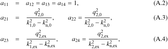
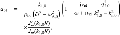
Appendix A: expression of the dispersion relation
The dispersion relation is  ,
with
,
with  given by the solution of the following determinant,
 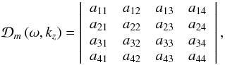 (A.1)with
 (A.5)
(A.5)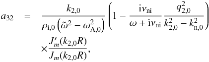 (A.6)
(A.6) (A.7)
(A.7) (A.8)
(A.8)![Mathematical equation: \appendix \setcounter{section}{1} \begin{eqnarray} a_{41} &=& k_{\rm 1,0} \left[ \frac{{\rm i} \nuin}{\omega + {\rm i} \nuin}\frac{1}{\rho_{\rm i,0} \left( \tilde{\omega}^2 - \omega_{\rm A,0}^2 \right)} \right. \nonumber \\ &&\times \left( 1 - \frac{{\rm i} \nuin}{\omega + {\rm i} \nuin}\frac{q_{2,0}^2}{k_{1,0}^2 - k_{\rm n,0}^2} \right) \nonumber \\ &&- \left. \frac{1}{\rho_{\rm n,0} \omega \left( \omega + {\rm i} \nuin \right)}\frac{q_{2,0}^2}{k_{1,0}^2 - k_{\rm n,0}^2} \right] \frac{J'_m(k_{\rm 1,0} R)}{J_m(k_{\rm 1,0} R)}, \end{eqnarray}](/articles/aa/full_html/2013/03/aa20576-12/aa20576-12-eq218.png) (A.9)
(A.9)![Mathematical equation: \appendix \setcounter{section}{1} \begin{eqnarray} a_{42} &=& k_{\rm 2,0} \left[ \frac{{\rm i} \nuin}{\omega + {\rm i} \nuin}\frac{1}{\rho_{\rm i,0}\left( \tilde{\omega}^2 - \omega_{\rm A,0}^2 \right)} \right. \nonumber \\ &&\times \left( 1 - \frac{{\rm i} \nuin}{\omega + {\rm i} \nuin}\frac{q_{2,0}^2}{k_{2,0}^2 - k_{\rm n,0}^2} \right) \nonumber \\ &&- \left. \frac{1}{\rho_{\rm n,0} \omega \left( \omega + {\rm i} \nuin \right)}\frac{q_{2,0}^2}{k_{2,0}^2 - k_{\rm n,0}^2} \right] \frac{J'_m(k_{\rm 2,0} R)}{J_m(k_{\rm 2,0} R)}, \end{eqnarray}](/articles/aa/full_html/2013/03/aa20576-12/aa20576-12-eq219.png) (A.10)
(A.10)![Mathematical equation: \appendix \setcounter{section}{1} \begin{eqnarray} a_{43} &=& k_{\rm 1,ex} \left[ \frac{{\rm i} \nuin}{\omega + {\rm i} \nuin}\frac{1}{\rho_{\rm i,ex}\left( \tilde{\omega}^2 - \omega_{\rm A,ex}^2 \right)} \right. \nonumber \\ &&\times \left( 1 - \frac{{\rm i} \nuin}{\omega + {\rm i} \nuin}\frac{q_{\rm 2,ex}^2}{k_{\rm 1,ex}^2 - k_{\rm n,ex}^2} \right) \nonumber \\ &&- \left. \frac{1}{\rho_{\rm n,ex} \omega \left( \omega + {\rm i} \nuin \right)}\frac{q_{\rm 2,ex}^2}{k_{\rm 1,ex}^2 - k_{\rm n,ex}^2} \right] \frac{H^{'(1)}_m(k_{\rm 1,ex} R)}{H^{(1)}_m(k_{\rm 1,ex} R)}, \end{eqnarray}](/articles/aa/full_html/2013/03/aa20576-12/aa20576-12-eq220.png) (A.11)
(A.11)![Mathematical equation: \appendix \setcounter{section}{1} \begin{eqnarray} a_{44} &=& k_{\rm 2,ex} \left[ \frac{{\rm i} \nuin}{\omega + {\rm i} \nuin}\frac{1}{\rho_{\rm i,ex}\left( \tilde{\omega}^2 - \omega_{\rm A,ex}^2 \right)} \right. \nonumber \\ &&\times \left( 1 - \frac{{\rm i} \nuin}{\omega + {\rm i} \nuin}\frac{q_{\rm 2,ex}^2}{k_{\rm 2,ex}^2 - k_{\rm n,ex}^2} \right) \nonumber \\ &&- \left. \frac{1}{\rho_{\rm n,ex} \omega \left( \omega + {\rm i} \nuin \right)}\frac{q_{\rm 2,ex}^2}{k_{\rm 2,ex}^2 - k_{\rm n,ex}^2} \right] \frac{H^{'(1)}_m(k_{\rm 2,ex} R)}{H^{(1)}_m(k_{\rm 2,ex} R)}\cdot \end{eqnarray}](/articles/aa/full_html/2013/03/aa20576-12/aa20576-12-eq221.png) (A.12)
(A.12)
All Figures
|
Fig. 1 a)ωR/ωk and b) ωI/ωk versus νni/ωk for the transverse kink (m = 1) mode with kzR = 0.1, ρi,0/ρi,ex = 3, cie,0/cA,0 = 0.2, and χ = 4. The solid line is the result obtained by numerically solving the dispersion relation in the absence of neutral pressure (Eq. (37)). The symbols are the approximate analytic results in the weak damping approximation (Eqs. (43) and (44)). |
| In the text | |
|
Fig. 2 Same as Fig. 1 but with χ = 20. The shaded area denotes the cut-off region given by Eq. (42). |
| In the text | |
|
Fig. 3 a)ωR/ωc,0 and b) ωI/ωc,0 versus νni/ωc,0 for the slow magnetoacoustic mode with χ = 4 and the rest of parameters the same as in Fig. 1. The solid line is the full result taking neutral pressure into account, while the dashed line is the result when neutral pressure is absent. |
| In the text | |
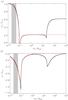 |
Fig. 4 Same as Fig. 3 but with χ = 20. The shaded area denotes the cut-off region given by Eq. (42). |
| In the text | |
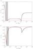 |
Fig. 5 Same as Fig. 4 but with χ = 100. |
| In the text | |
Current usage metrics show cumulative count of Article Views (full-text article views including HTML views, PDF and ePub downloads, according to the available data) and Abstracts Views on Vision4Press platform.
Data correspond to usage on the plateform after 2015. The current usage metrics is available 48-96 hours after online publication and is updated daily on week days.
Initial download of the metrics may take a while.