| Issue |
A&A
Volume 551, March 2013
|
|
|---|---|---|
| Article Number | A84 | |
| Number of page(s) | 13 | |
| Section | Astrophysical processes | |
| DOI | https://doi.org/10.1051/0004-6361/201220511 | |
| Published online | 27 February 2013 | |
Isotropic inelastic and superelastic collisional rates in a multiterm atom
1
Instituto de Astrofísica de Canarias, C. vía Láctea s/n, 38205 La Laguna,
Tenerife, Spain
e-mail:
This email address is being protected from spambots. You need JavaScript enabled to view it.
2
Departamento de Astrofísica, Facultad de Física, Universidad de La
Laguna, 38206,
La Laguna, Tenerife,
Spain
3
Dipartimento di Fisica e Astronomia, Università di
Firenze, Largo E. Fermi
2, 50125
Firenze,
Italy
4
Consejo Superior de Investigaciones Científicas,
Spain
Received:
6
October
2012
Accepted:
4
November
2012
Abstract
The spectral line polarization of the radiation emerging from a magnetized astrophysical plasma depends on the state of the atoms within the medium, whose determination requires considering the interactions between the atoms and the magnetic field, between the atoms and photons (radiative transitions), and between the atoms and other material particles (collisional transitions). In applications within the framework of the multiterm model atom (which accounts for quantum interference between magnetic sublevels pertaining either to the same J-level or to different J-levels within the same term) collisional processes are generally neglected when solving the master equation for the atomic density matrix. This is partly due to the lack of experimental data and/or of approximate theoretical expressions for calculating the collisional transfer and relaxation rates (in particular the rates for interference between sublevels pertaining to different J-levels, and the depolarizing rates due to elastic collisions). In this paper we formally define and investigate the transfer and relaxation rates due to isotropic inelastic and superelastic collisions that enter the statistical equilibrium equations for the atomic density matrix of a multiterm atom. Under the hypothesis that the interaction between the collider and the atom can be described by a dipolar operator, we provide expressions that relate the collisional rates for interference between different J-levels to the usual collisional rates for J-level populations, for which experimental data or approximate theoretical expressions are generally available. We show that the rates for populations and interference within the same J-level reduce to those previously obtained for the multilevel model atom (where quantum interference is assumed to be present only between magnetic sublevels pertaining to any given J-level). Finally, we apply the general equations to the case of a two-term atom with unpolarized lower term, illustrating the impact of inelastic and superelastic collisions on the scattering line polarization through radiative transfer calculations in a slab of stellar atmospheric plasma anisotropically illuminated by the photospheric radiation field.
Key words: atomic processes / line: formation / polarization / radiative transfer / scattering / stars: atmospheres
© ESO, 2013
1. Introduction
The intensity and polarization of the spectral line radiation emerging from an astrophysical plasma depends on the population and atomic polarization (i.e., population imbalances and quantum interference between different magnetic sublevels) of the lower and upper line levels at each spatial point along the line of sight (LOS). Determining the population and atomic polarization of such levels requires considering the interactions between the atoms and photons (radiative transitions) and between the atoms and other material particles, such as electrons, atoms, and ions (collisional transitions). This problem can be very complex, especially when it comes to modeling the spectral line polarization produced by the joint action of anisotropic radiation pumping and the Hanle and Zeeman effects in multilevel systems.
Within the framework of the density-matrix theory of spectral line polarization described in the monograph by Landi Degl’Innocenti & Landolfi (2004; hereafter LL04), it is possible to develop a consistent set of equations for multilevel systems, either by neglecting (multilevel model atom) or considering (multiterm model atom) quantum interference between pairs of magnetic sublevels pertaining to different J-levels (with J the level’s total angular momentum value). The relevant equations are the radiative transfer equation for the Stokes parameters (where the coefficients of the emission vector and of the propagation matrix depend on the values of the atomic density matrix) and the master equation for the atomic density matrix (which includes both radiative and collisional rates).
While for the multilevel model atom LL04 derived the expressions for both radiative and collisional rates (assuming isotropic collisions), for the multiterm model atom they only provide the expressions for the radiative rates. The aim of this paper is to formally define the collisional rates for a multiterm atom, and to find their relevant properties, focusing our attention only on isotropic inelastic and superelastic collisions. The treatment of elastic collisions in a multiterm atom is actually more complicated, and will not be treated here. Such collisions (e.g., with neutral hydrogen atoms) tend to equalize the populations of the sublevels pertaining to any given J-level and to destroy any quantum interference between pairs of them. A similar depolarizing role may be caused by inelastic and superelastic collisions between the J-levels pertaining to any given term, especially when such J-levels are very close in energy (see Bommier 2009, for the hydrogen case). For the sake of simplicity, the latter type of collision will also be neglected, the investigation being limited to inelastic and superelastic collisions between different terms.
In the main body of this paper, we provide suitable expressions for the transfer and relaxation rates caused by isotropic inelastic and superelastic collisions, taking the possibility of atomic polarization in all the terms of the model atom into account. Particular attention is given to the collisional transfer and relaxation rates for interference between magnetic sublevels pertaining to different J-levels, the physical ingredient that cannot be accounted for with a multilevel model atom. Since there are basically no experimental data for such rates, we provide approximate expressions that relate such rates to the usual collisional rates that describe transitions between different J-levels (for which experimental data or theoretical expressions are generally available). As a consistency proof of our derivation, we show that the transfer and relaxation rates for populations and interference between pairs of magnetic sublevels pertaining to the same J-level reduce to those derived by LL04 for the multilevel atom case.
In the last section we present an illustrative application of the theoretical scheme developed here. We consider a two-term atom with unpolarized lower term, and we show the sensitivity to the collisional rates of the linear polarization of the radiation emerging from a slab of given optical depth, located at a given height above the “surface” of a solar-like star, and illuminated by its photospheric radiation field.
2. Transfer rate due to inelastic collisions
We consider a multiterm atom (see Sects. 7.5 and 7.6 of LL04) in the absence of magnetic
fields, and we describe it by means of the density matrix elements
ρβLS(JM,J′M′),
with J the total angular momentum, M its projection along
the quantization axis, L the orbital angular momentum, S
the spin, and β the electronic configuration. This atomic model accounts
for quantum interference (or coherence) between pairs of magnetic sublevels pertaining
either to the same J-level or to different J-levels of the
same term (J-state interference). We also work using the multipole moments
of the density matrix (or spherical statistical tensors), defined by the equation
 (1)Although
collisional processes can be very efficient in coupling J-levels pertaining
to the same term, in this investigation we only consider collisional processes coupling
populations and coherence pertaining to different terms.
(1)Although
collisional processes can be very efficient in coupling J-levels pertaining
to the same term, in this investigation we only consider collisional processes coupling
populations and coherence pertaining to different terms.
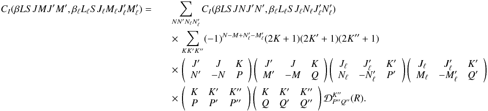
In a given, although arbitrary, reference system, transfer processes due to inelastic
collisions contribute to the time evolution of a particular density matrix element according
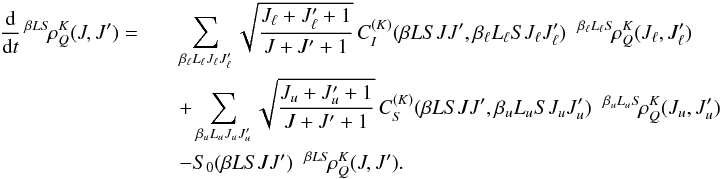
to the equation  (2)where
CI is the inelastic collision transfer rate
and where the quantum numbers
(βℓLℓS)
denote any term having energy lower than the term (βLS)1. In a new reference system, obtained from the old one by the rotation
R, recalling the transformation law (see Eq. (3.95) of LL04)
(2)where
CI is the inelastic collision transfer rate
and where the quantum numbers
(βℓLℓS)
denote any term having energy lower than the term (βLS)1. In a new reference system, obtained from the old one by the rotation
R, recalling the transformation law (see Eq. (3.95) of LL04)
![Mathematical equation: \begin{eqnarray} \left[ \rho_{\beta L S}(J M, J^{\prime} M^{\prime}) \right]_{\rm new} = \sum_{N N^{\prime}} {\mathcal D}^J_{NM}(R)^{\ast} \, {\mathcal D}^{J^{\prime}}_{N^{\prime} M^{\prime}}(R) \left[ \rho_{\beta L S}(J N, J^{\prime} N^{\prime}) \right]_{\rm old}, \label{Eq:rot1} \end{eqnarray}](/articles/aa/full_html/2013/03/aa20511-12/aa20511-12-eq13.png) (3)with
(3)with
 the rotation matrices, and
its inverse
the rotation matrices, and
its inverse ![Mathematical equation: \begin{eqnarray} \left[ \rho_{\beta L S}(J M, J^{\prime} M^{\prime}) \right]_{\rm old} = \sum_{N N^{\prime}} {\mathcal D}^J_{M N}(R) \, {\mathcal D}^{J^{\prime}}_{M^{\prime} N^{\prime}}(R)^{\ast} \left[ \rho_{\beta L S}(J N, J^{\prime} N^{\prime}) \right]_{\rm new}, \label{Eq:rot2} \end{eqnarray}](/articles/aa/full_html/2013/03/aa20511-12/aa20511-12-eq15.png) (4)we
have
(4)we
have ![Mathematical equation: \begin{eqnarray} \label{Eq:CI_std_new} \frac{\rm d}{{\rm d} t} \left[ \rho_{\beta L S}(J M, J^{\prime} M^{\prime}) \right]_{\rm new} = \sum_{\beta_{\ell} L_{\ell} J_{\ell} M_{\ell} J_{\ell}^{\prime} M_{\ell}^{\prime}} && \left\{ \sum_{N N_{\phantom{\ell}}^{\prime} N_{\ell} N_{\ell}^{\prime}} {\mathcal D}^{J}_{N M}(R)^{\ast} \, {\mathcal D}^{J^{\prime}}_{N^{\prime} M^{\prime}}(R) \, {\mathcal D}^{J_{\ell}}_{N_{\ell} M_{\ell}}(R) \, {\mathcal D}^{J^{\prime}_{\ell}}_{N^{\prime}_{\ell} M^{\prime}_{\ell}}(R)^{\ast} \, C_I(\beta L S J N J^{\prime} N^{\prime}, \beta_{\ell} L_{\ell} S J_{\ell} N_{\ell} J_{\ell}^{\prime} N_{\ell}^{\prime}) \right\} \nonumber\\ && \times \, \left[ \rho_{\beta_{\ell} L_{\ell} S}(J_{\ell} M_{\ell}, J_{\ell}^{\prime} M_{\ell}^{\prime}) \right]_{\rm new}. \end{eqnarray}](/articles/aa/full_html/2013/03/aa20511-12/aa20511-12-eq16.png) (5)The
assumption of isotropic collisions implies that all the quantization directions are
equivalent, so that Eqs. (2) and (5) have to be identical. It follows that the
collisional rates must satisfy the relation
(5)The
assumption of isotropic collisions implies that all the quantization directions are
equivalent, so that Eqs. (2) and (5) have to be identical. It follows that the
collisional rates must satisfy the relation  (6)After coupling through
Eq. (A.10) the rotation matrices
(6)After coupling through
Eq. (A.10) the rotation matrices
 and
and
 , as well as the rotation matrices
 and
and
 , and using the complex
conjugate of Eq. (A.11) on the ensuing
expression, Eq. (6) takes the form
, and using the complex
conjugate of Eq. (A.11) on the ensuing
expression, Eq. (6) takes the form
 (7)As
the righthand side of Eq. (7) must be
independent of the rotation R, the index K′′
can only take the value K′′ = 0. This implies
K = K′,
P = −P′, and
Q = −Q′. Using Eq. (A.4), we obtain
(7)As
the righthand side of Eq. (7) must be
independent of the rotation R, the index K′′
can only take the value K′′ = 0. This implies
K = K′,
P = −P′, and
Q = −Q′. Using Eq. (A.4), we obtain 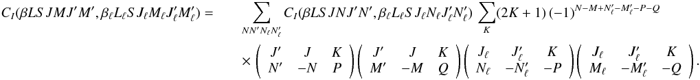 (8)
(8)
2.1. Multipole components of the inelastic collision transfer rate
Introducing the multipole components of the inelastic collision transfer rate, defined by
the equation2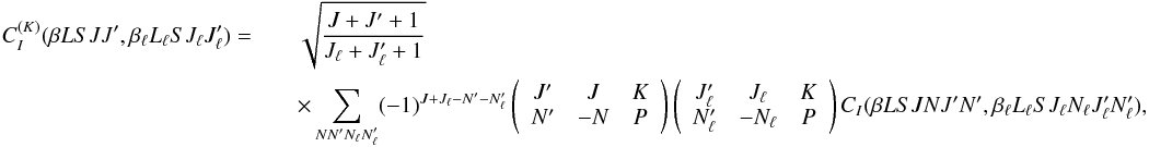 (9)and
making use of Eqs. (A.1) and (A.2), Eq. (8) can be written in the form
(9)and
making use of Eqs. (A.1) and (A.2), Eq. (8) can be written in the form 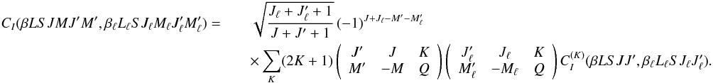 (10)Substituting
Eq. (10) into Eq. (2), and recalling the definition of the
multipole moments of the density matrix (see Eq. (1)), with the help of Eq. (A.3),
we find the following equation for the spherical statistical tensors
(10)Substituting
Eq. (10) into Eq. (2), and recalling the definition of the
multipole moments of the density matrix (see Eq. (1)), with the help of Eq. (A.3),
we find the following equation for the spherical statistical tensors
 (11)Taking the complex
conjugate of Eq. (2) and recalling that
ρβLS(JM,J′M′)∗ = ρβLS(J′M′,JM),
we have
(11)Taking the complex
conjugate of Eq. (2) and recalling that
ρβLS(JM,J′M′)∗ = ρβLS(J′M′,JM),
we have  (12)and therefore, using Eqs.
(A.1) and (A.2),
(12)and therefore, using Eqs.
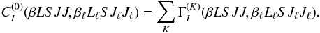
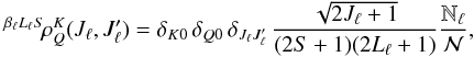
(A.1) and (A.2),  (13)Setting
K = 0 in Eq. (9), and
using Eq. (A.4), we obtain
(13)Setting
K = 0 in Eq. (9), and
using Eq. (A.4), we obtain  (14)where the transfer rate
CI(βLSJNJN,βℓLℓSJℓNℓJℓNℓ)
is the usual (inelastic) collisional rate for the transition from the lower magnetic
sublevel
| βℓLℓSJℓNℓ ⟩
to the upper magnetic sublevel | βLSJN ⟩, generally indicated in the
literature with the notation
(14)where the transfer rate
CI(βLSJNJN,βℓLℓSJℓNℓJℓNℓ)
is the usual (inelastic) collisional rate for the transition from the lower magnetic
sublevel
| βℓLℓSJℓNℓ ⟩
to the upper magnetic sublevel | βLSJN ⟩, generally indicated in the
literature with the notation  .
Since this rate is non-negative, the 0-rank multipole component is also non-negative.
.
Since this rate is non-negative, the 0-rank multipole component is also non-negative.
2.2. Relations with the collisional rates for J-level populations
In most cases, the only collisional rates for which experimental data, or approximate
analytical expressions, are available are the collisional rates connecting the populations
of different J-levels (following the notation generally used in the
literature, these rates will be indicated through the symbols
 and
and  ,
the indices I and S standing for “inelastic” and
“superelastic”, respectively). It is important therefore to find suitable relations
between such rates and the collisional rates introduced in this paper for a multiterm
atom.
,
the indices I and S standing for “inelastic” and
“superelastic”, respectively). It is important therefore to find suitable relations
between such rates and the collisional rates introduced in this paper for a multiterm
atom.
Observing that  (15)from Eq. (14) we immediately have
  (16)In Eq. (6), if we couple through Eq. (A.10) the rotation matrices
and
(16)In Eq. (6), if we couple through Eq. (A.10) the rotation matrices
and
 , as well as the rotation
matrices and
, as well as the rotation
matrices and
 , by requiring
that the ensuing expression is independent of the rotation R, we find the
relation
, by requiring
that the ensuing expression is independent of the rotation R, we find the
relation 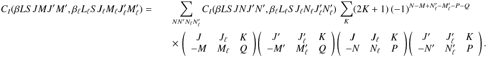 (17)Defining
a different set of multipole components of the inelastic collision transfer rate through
the equation
(17)Defining
a different set of multipole components of the inelastic collision transfer rate through
the equation  (18)Equation
(17) can be written in the form
(18)Equation
(17) can be written in the form
 (19)As
pointed out in LL04 for the multilevel atom case, this decomposition of the collisional
rate has an interesting physical interpretation, because it shows that the interaction
between the atomic system and the collider can be described by a sum of tensor operators
of rank K acting on the state vectors of the atom. Starting from Eq.
(9) and using Eq. (A.8), after some algebra the following
relation between the multipole components
(19)As
pointed out in LL04 for the multilevel atom case, this decomposition of the collisional
rate has an interesting physical interpretation, because it shows that the interaction
between the atomic system and the collider can be described by a sum of tensor operators
of rank K acting on the state vectors of the atom. Starting from Eq.
(9) and using Eq. (A.8), after some algebra the following
relation between the multipole components  and
and
 can be found:
  (20)For the
K = 0 multipole component, using Eq. (A.7), we have (cf. Appendix A4 of LL04)
(20)For the
K = 0 multipole component, using Eq. (A.7), we have (cf. Appendix A4 of LL04)
 (21)When the interaction can
be described through just one operator of rank
(21)When the interaction can
be described through just one operator of rank  ,
then
,
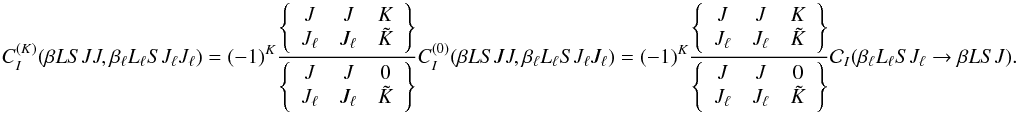
then  (22)The multipole component
of rank K of the diagonal rates
(J = J′ and
(22)The multipole component
of rank K of the diagonal rates
(J = J′ and
 ) is thus
related to the multipole component of rank 0 by the equation (cf. Appendix A4 of LL04)
) is thus
related to the multipole component of rank 0 by the equation (cf. Appendix A4 of LL04)
 (23)A similar relation
for the nondiagonal rates (describing the transfer of J-state
interference due to inelastic collisions) cannot be obtained through symmetry arguments
alone. Such a relation can, however, be derived if some simplifying hypotheses on the
interaction between the atoms and perturbers are introduced. It is well known that in the
case of electrons with much higher energy than the threshold energy (i.e. under the
so-called Born approximation), the Hamiltonian describing the electron-atom interaction
depends on the dynamical variables of the atom only through the dipole operator (a tensor
of rank
(23)A similar relation
for the nondiagonal rates (describing the transfer of J-state
interference due to inelastic collisions) cannot be obtained through symmetry arguments
alone. Such a relation can, however, be derived if some simplifying hypotheses on the
interaction between the atoms and perturbers are introduced. It is well known that in the
case of electrons with much higher energy than the threshold energy (i.e. under the
so-called Born approximation), the Hamiltonian describing the electron-atom interaction
depends on the dynamical variables of the atom only through the dipole operator (a tensor
of rank  ). A collisional process in an
optically allowed transition can thus be treated, in a first approximation, as a radiative
transition, and the collisional rate can be expressed through the oscillator strength of
the same transition (e.g. Seaton 1962; Van Regemorter 1962).
). A collisional process in an
optically allowed transition can thus be treated, in a first approximation, as a radiative
transition, and the collisional rate can be expressed through the oscillator strength of
the same transition (e.g. Seaton 1962; Van Regemorter 1962).
For more insight on the nondiagonal rates  , we assume that the
electron-atom interaction is described by a dipolar operator, and we proceed by analogy
with the multiterm atom radiative transfer rate due to absorption processes
(TA). Setting
Kr = 0 (i.e. assuming an isotropic
radiation field) in Eq. (7.45a) of LL04, we have
, we assume that the
electron-atom interaction is described by a dipolar operator, and we proceed by analogy
with the multiterm atom radiative transfer rate due to absorption processes
(TA). Setting
Kr = 0 (i.e. assuming an isotropic
radiation field) in Eq. (7.45a) of LL04, we have 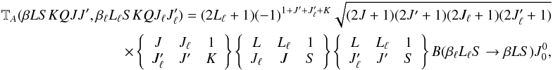 (24)where
 is the
angle-averaged incident radiation field, and
B(βℓLℓS → βLS)
is the Einstein coefficient for absorption from the lower term
(βℓLℓS)
to the upper term (βLS). We recall that this quantity is connected to the
Einstein coefficients for the individual transitions between fine structure
J-levels of the multiplet by the relation (see Eq. (7.57a) of LL04)
is the
angle-averaged incident radiation field, and
B(βℓLℓS → βLS)
is the Einstein coefficient for absorption from the lower term
(βℓLℓS)
to the upper term (βLS). We recall that this quantity is connected to the
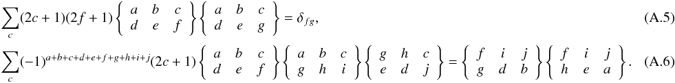
Einstein coefficients for the individual transitions between fine structure
J-levels of the multiplet by the relation (see Eq. (7.57a) of LL04)
 (25)which implies
(using Eq. (A.5))3
(25)which implies
(using Eq. (A.5))3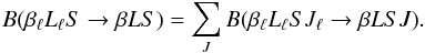 (26)By analogy with Eq.
(26), we define an inelastic collisional
rate for the transition from the lower to the upper term
(26)By analogy with Eq.
(26), we define an inelastic collisional
rate for the transition from the lower to the upper term
 through the equation
 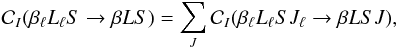 (27)where the sum is extended
to all the J-levels of the upper term to which a given
J-level of the lower term can be connected through an electric dipole
transition. By analogy with Eq. (24), and
taking the multiplying factor introduced in Eq. (9) into account (see footnote 2), we can write
(27)where the sum is extended
to all the J-levels of the upper term to which a given
J-level of the lower term can be connected through an electric dipole
transition. By analogy with Eq. (24), and
taking the multiplying factor introduced in Eq. (9) into account (see footnote 2), we can write 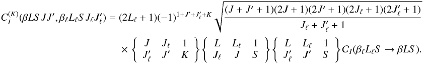 (28)This
equation can be used to calculate the multipole components of the inelastic collision
transfer rates for J-state interference from the values of the usual
inelastic collisional rates for J-level populations. As a proof of the
consistency of Eq. (28), we observe that
the 0-rank multipole component is given by
(28)This
equation can be used to calculate the multipole components of the inelastic collision
transfer rates for J-state interference from the values of the usual
inelastic collisional rates for J-level populations. As a proof of the
consistency of Eq. (28), we observe that
the 0-rank multipole component is given by  (29)which is the
analogous to Eq. (25), while using Eqs.
(A.7) and (29), the diagonal terms are given by
(29)which is the
analogous to Eq. (25), while using Eqs.
(A.7) and (29), the diagonal terms are given by 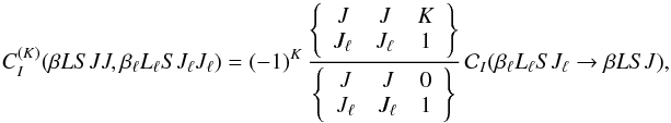 (30)which corresponds
to Eq. (23) for
.
(30)which corresponds
to Eq. (23) for
.
3. Transfer rate due to superelastic collisions
A similar reasoning can be followed for the transfer rates due to superelastic collisions.
These transfer processes contribute to the time evolution of a particular density matrix
element according to the equation  (31)where
CS is the superelastic collision transfer
rate and where the quantum numbers
(βuLuS)
denote any term having energy higher than the term (βLS). Following the
same steps as in Sect. 2, it can be shown that under
the assumption of isotropic collisions, the transfer rate
CS can be written in the form
(31)where
CS is the superelastic collision transfer
rate and where the quantum numbers
(βuLuS)
denote any term having energy higher than the term (βLS). Following the
same steps as in Sect. 2, it can be shown that under
the assumption of isotropic collisions, the transfer rate
CS can be written in the form 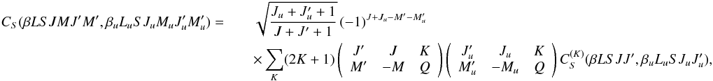 (32)where
the multipole components of the superelastic collision transfer rate,
(32)where
the multipole components of the superelastic collision transfer rate,
 ,
are defined by the equation
,
are defined by the equation 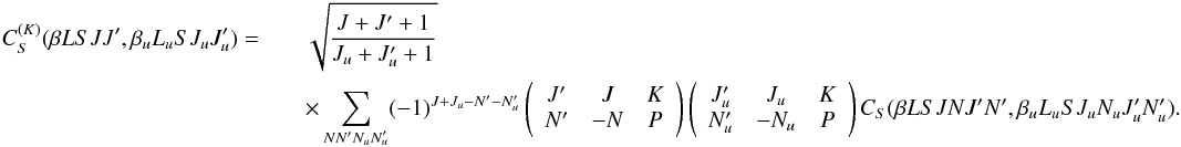 (33)By
substituting Eq. (32) into Eq. (31), and recalling Eq. (1), we find the following equation for the
spherical statistical tensors
(33)By
substituting Eq. (32) into Eq. (31), and recalling Eq. (1), we find the following equation for the
spherical statistical tensors  (34)The 0-rank multipole
component is given by
(34)The 0-rank multipole
component is given by  (35)where
 is the usual superelastic collisional rate for the transition from the upper level
| βuLuSJu ⟩
to the lower level | βLSJ ⟩. When the interaction between the atomic
system and the colliders can be described by means of a single operator of rank
,
it can be shown that the multipole components of rank K of the diagonal
rates (J = J′ and
is the usual superelastic collisional rate for the transition from the upper level
| βuLuSJu ⟩
to the lower level | βLSJ ⟩. When the interaction between the atomic
system and the colliders can be described by means of a single operator of rank
,
it can be shown that the multipole components of rank K of the diagonal
rates (J = J′ and
 ) are related to
the multipole components of rank 0 by the equation
) are related to
the multipole components of rank 0 by the equation 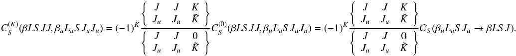 (36)As discussed in the
previous section for the case of inelastic collisions, a similar relation for the
nondiagonal rates (describing the transfer of J-state interference due to
superelastic collisions) can be derived under the assumption that the electron-atom
interaction is described by a dipolar operator. By analogy with the expression of the
multiterm atom radiative transfer rate due to stimulated emission processes
(TS, see Eq. (7.45c) of LL04) in the presence of an
isotropic incident field, we find the following relation
(36)As discussed in the
previous section for the case of inelastic collisions, a similar relation for the
nondiagonal rates (describing the transfer of J-state interference due to
superelastic collisions) can be derived under the assumption that the electron-atom
interaction is described by a dipolar operator. By analogy with the expression of the
multiterm atom radiative transfer rate due to stimulated emission processes
(TS, see Eq. (7.45c) of LL04) in the presence of an
isotropic incident field, we find the following relation 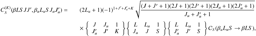 (37)where
we have introduced the superelastic collisional rate for the transition from the upper to
the lower term
(37)where
we have introduced the superelastic collisional rate for the transition from the upper to
the lower term  ,
defined by
,
defined by 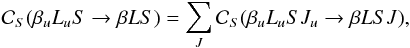 (38)the sum being extended to
all the J-levels of the lower term to which a given
J-level of the upper term can be connected through an electric dipole
transition4.
(38)the sum being extended to
all the J-levels of the lower term to which a given
J-level of the upper term can be connected through an electric dipole
transition4.
4. Relaxation rates due to inelastic and superelastic collisions
In a given reference system, relaxation processes due to inelastic and superelastic
collisions contribute to the time evolution of a particular density-matrix element via an
equation of the form ![Mathematical equation: \begin{equation} \frac{\rm d}{{\rm d} t} \, \rho_{\beta L S}(J M, J^{\prime}M^{\prime}) = - \sum_{J^{\prime \prime} M^{\prime \prime}} \left[ f(\beta L S J M J^{\prime} M^{\prime} J^{\prime \prime} M^{\prime \prime}) \, \rho_{\beta L S}(J M, J^{\prime \prime} M^{\prime \prime}) + g(\beta L S J M J^{\prime} M^{\prime} J^{\prime \prime} M^{\prime \prime}) \, \rho_{\beta L S}(J^{\prime \prime} M^{\prime \prime}, J^{\prime} M^{\prime}) \right]. \label{Eq:RLX_std1} \end{equation}](/articles/aa/full_html/2013/03/aa20511-12/aa20511-12-eq92.png) (39)The conjugation property of
the density-matrix elements
(ρβLS(JM,J′M′)∗ = ρβLS(J′M′,JM))
requires that
(39)The conjugation property of
the density-matrix elements
(ρβLS(JM,J′M′)∗ = ρβLS(J′M′,JM))
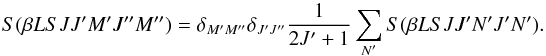
requires that  (40)so that Eq. (39) can be written in the form
 ![Mathematical equation: \begin{equation} \frac{\rm d}{{\rm d} t} \, \rho_{\beta L S}(J M, J^{\prime}M^{\prime}) = - \sum_{J^{\prime \prime} M^{\prime \prime}} \left[ \frac{1}{2} S(\beta L S J M J^{\prime} M^{\prime} J^{\prime \prime} M^{\prime \prime}) \, \rho_{\beta L S}(J M, J^{\prime \prime} M^{\prime \prime}) + \frac{1}{2} S(\beta L S J^{\prime} M^{\prime} J M J^{\prime \prime} M^{\prime \prime})^{\ast} \, \rho_{\beta L S}(J^{\prime \prime} M^{\prime \prime}, J^{\prime} M^{\prime}) \right]. \label{Eq:RLX_std2} \end{equation}](/articles/aa/full_html/2013/03/aa20511-12/aa20511-12-eq95.png) (41)In a new reference system,
obtained from the old one by the rotation R, recalling Eqs. (3) and (4), we have
(41)In a new reference system,
obtained from the old one by the rotation R, recalling Eqs. (3) and (4), we have ![Mathematical equation: \begin{eqnarray} \label{Eq:RLX_std2_new} \frac{\rm d}{{\rm d} t} \left[ \rho_{\beta L S}(J M, J^{\prime} M^{\prime}) \right]_{\rm new} = -\sum_{J^{\prime \prime} M^{\prime \prime} M^{\prime \prime \prime}} \Bigg\{ && \frac{1}{2} \sum_{N N^{\prime} N^{\prime \prime}} {\mathcal D}^{J}_{N M}(R)^{\ast} \, {\mathcal D}^{J^{\prime}}_{N^{\prime} M^{\prime}}(R) \, S(\beta L S J N J^{\prime} N^{\prime} J^{\prime \prime} N^{\prime \prime}) \nonumber\\ && \phantom{\Bigg\{ } \quad \quad \quad \times \, {\mathcal D}^{J}_{N M^{\prime \prime \prime}}(R) \, {\mathcal D}^{J^{\prime \prime}}_{N^{\prime \prime} M^{\prime \prime}} (R)^{\ast} \, \left[ \rho_{\beta L S}(J M^{\prime \prime \prime}, J^{\prime \prime} M^{\prime \prime}) \right]_{\rm new} \nonumber\\ && \phantom{\Bigg\{ } \!\!\!\!\!\!\!\!\!\! + \, \frac{1}{2} \sum_{N N^{\prime} N^{\prime \prime}} {\mathcal D}^{J}_{N M}(R)^{\ast} \, {\mathcal D}^{J^{\prime}}_{N^{\prime} M^{\prime}}(R) \, S(\beta L S J^{\prime} N^{\prime} J N J^{\prime \prime} N^{\prime \prime})^{\ast} \nonumber\\ && \phantom{\Bigg\{ } \quad \quad \quad \times \, {\mathcal D}^{J^{\prime \prime}}_{N^{\prime \prime} M^{\prime \prime}} (R) \, {\mathcal D}^{J^{\prime}}_{N^{\prime} M^{\prime \prime \prime}} (R)^{\ast} \, \left[ \rho_{\beta L S}(J^{\prime \prime} M^{\prime \prime}, J^{\prime} M^{\prime \prime \prime}) \right]_{\rm new} \Bigg\} . \end{eqnarray}](/articles/aa/full_html/2013/03/aa20511-12/aa20511-12-eq96.png) (42)Due
to the isotropy of collisions, Eqs. (41) and
(42) must be identical, which implies
(42)Due
to the isotropy of collisions, Eqs. (41) and
(42) must be identical, which implies
 (43)regardless of the
rotation R. This requires the rate
S(βLSJNJ′N′J′′N′′)
to be independent of the quantum number N (if not, the righthand side of
Eq. (43) would not be zero for
M ≠ M′′′, no matter the rotation
R). We can thus carry out the summation over N via Eq.
(A.9) to get (with the help of Eq. (A.10))
(43)regardless of the
rotation R. This requires the rate
S(βLSJNJ′N′J′′N′′)
to be independent of the quantum number N (if not, the righthand side of
Eq. (43) would not be zero for
M ≠ M′′′, no matter the rotation
R). We can thus carry out the summation over N via Eq.
(A.9) to get (with the help of Eq. (A.10))  (44)Since
the righthand side of Eq. (44) must be
independent of the rotation R, index K can only take the
value K = 0, which implies Q = P = 0,
N′ = N′′,
M′ = M′′, and
J′ = J′′ from Eq. (A.4). We thus obtain
(44)Since
the righthand side of Eq. (44) must be
independent of the rotation R, index K can only take the
value K = 0, which implies Q = P = 0,
N′ = N′′,
M′ = M′′, and
J′ = J′′ from Eq. (A.4). We thus obtain
 (45)Substitution into Eq.
(41) gives
(45)Substitution into Eq.
(41) gives 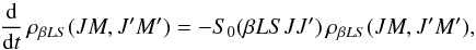 (46)or, in the spherical
statistical tensor representation,
(46)or, in the spherical
statistical tensor representation, 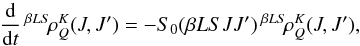 (47)where we have
introduced the collisional relaxation rate
(47)where we have
introduced the collisional relaxation rate
![Mathematical equation: \begin{equation} S_0(\beta L S J J^{\prime}) = \frac{1}{2} \left[ \frac{1}{2J^{\prime} + 1} \sum_{M^{\prime}} S(\beta L S J J^{\prime} M^{\prime} J^{\prime} M^{\prime}) + \frac{1}{2J + 1} \sum_M S(\beta L S J^{\prime} J M J M)^{\ast} \right]. \end{equation}](/articles/aa/full_html/2013/03/aa20511-12/aa20511-12-eq109.png) (48)The diagonal element
(48)The diagonal element
![Mathematical equation: \begin{equation} S_0(\beta L S J J) = \frac{1}{2J + 1} \frac{1}{2} \sum_M \left[ S(\beta L S J J M J M) + S(\beta L S J J M J M)^{\ast} \right] = \frac{1}{2J +1} {\rm Re} \left[ \sum_M S(\beta L S J J M J M)) \right] \end{equation}](/articles/aa/full_html/2013/03/aa20511-12/aa20511-12-eq110.png) (49)coincides
with the one defined in LL04 for the case of a multilevel atom.
(49)coincides
with the one defined in LL04 for the case of a multilevel atom.
As shown in LL04, the diagonal element
S0(βLSJJ), which represents the relaxation
rate of populations and interference between magnetic sublevels pertaining to the same
J-level (see Eqs. (46)
and (47)), is connected to the 0-rank
multipole components of the inelastic and superelastic collision transfer rates by the
equation  (50)To obtain a similar
relation for the nondiagonal elements
(S0(βLSJJ′) with
J ≠ J′), which represent the relaxation rate
of J-state interference due to inelastic and superelastic collisions, we
make the assumption, also in this case, that the interaction between the atoms and colliders
is described by a dipolar operator, and we proceed by analogy with the multiterm atom
radiative relaxation rates due to absorption (RA) and stimulated
emission (RS) processes (see Eqs. (7.46a) and (7.46c) of LL04).
Assuming an isotropic incident radiation field (i.e. setting
Kr = 0), such radiative rates assume the
simple form
(50)To obtain a similar
relation for the nondiagonal elements
(S0(βLSJJ′) with
J ≠ J′), which represent the relaxation rate
of J-state interference due to inelastic and superelastic collisions, we
make the assumption, also in this case, that the interaction between the atoms and colliders
is described by a dipolar operator, and we proceed by analogy with the multiterm atom
radiative relaxation rates due to absorption (RA) and stimulated
emission (RS) processes (see Eqs. (7.46a) and (7.46c) of LL04).
Assuming an isotropic incident radiation field (i.e. setting
Kr = 0), such radiative rates assume the
simple form 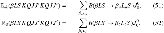 Introducing
the inelastic and superelastic collisional rates for transitions between different terms
(see Eqs. (27) and (38)), we have
Introducing
the inelastic and superelastic collisional rates for transitions between different terms
(see Eqs. (27) and (38)), we have 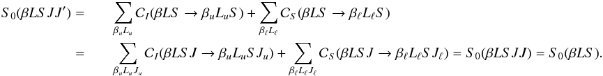 (53)The
relaxation rate of J-state interference due to inelastic and superelastic
collisions thus coincides with the relaxation rate of J-level populations
and of interference between magnetic sublevels pertaining to the same
J-level. This rate, on the other hand, does not depend on the quantum
number J, and is thus identical for all the J-levels of a
given term.
(53)The
relaxation rate of J-state interference due to inelastic and superelastic
collisions thus coincides with the relaxation rate of J-level populations
and of interference between magnetic sublevels pertaining to the same
J-level. This rate, on the other hand, does not depend on the quantum
number J, and is thus identical for all the J-levels of a
given term.
When collected together transfer and relaxation rates, the statistical equilibrium
equations for the spherical statistical tensors can be written in the form
 (54)
(54)
5. Application to the case of a two-term atom with unpolarized lower term
We consider a two-term atom and denote the quantum numbers characterizing the lower and
upper term by
(βℓLℓS)
and
(βuLuS),
respectively. The time evolution of the spherical statistical tensors of the upper term,
when taking both radiative (see Eq. (10.115) of LL04) and collisional (inelastic and
superelastic collisions only) processes into account is described by the equation
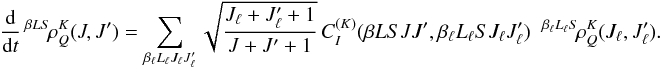
![Mathematical equation: \begin{eqnarray} \frac{\rm d}{{\rm d} t} \, ^{\beta_u L_u S} \! \rho^K_Q(J_u, J_u^{\prime}) = && - 2 \pi {\rm i} \sum_{K^{\prime} Q^{\prime} J_u^{\prime \prime} J_u^{\prime \prime \prime}} N_{\beta_u L_u S}(K Q J_u J_u^{\prime}, K^{\prime} Q^{\prime} J_u^{\prime \prime} J_u^{\prime \prime \prime})\;\; ^{\beta_u L_u S} \! \rho^{K^{\prime}}_{Q^{\prime}} (J_u^{\prime \prime}, J_u^{\prime \prime \prime}) \nonumber\\ && + \sum_{K^{\prime} Q^{\prime} J_{\ell} J_{\ell}^{\prime}} \mathbb{T}_A(\beta_u L_u S K Q J_u J_u^{\prime}, \beta_{\ell} L_{\ell} S K^{\prime} Q^{\prime} J_{\ell} J_{\ell}^{\prime}) \;\; ^{\beta_{\ell} L_{\ell} S} \! \rho^{K^{\prime}}_{Q^{\prime}} (J_{\ell}, J_{\ell}^{\prime}) \nonumber\\ && - \sum_{K^{\prime} Q^{\prime} J_u^{\prime \prime} J_u^{\prime \prime \prime}} \bigg[ \mathbb{R}_E(\beta_u L_u S K Q J_u J_u^{\prime} K^{\prime} Q^{\prime} J_u^{\prime \prime} J_u^{\prime \prime \prime}) \nonumber\\ && \qquad \qquad + \mathbb{R}_S(\beta_u L_u S K Q J_u J_u^{\prime} K^{\prime} Q^{\prime} J_u^{\prime \prime} J_u^{\prime \prime \prime}) \bigg] \;\; ^{\beta_u L_u S} \! \rho^{K^{\prime}}_{Q^{\prime}} (J_u^{\prime \prime}, J_u^{\prime \prime \prime}) \nonumber\\ && + \sum_{J_{\ell} J_{\ell}^{\prime}} \sqrt{\frac{J_{\ell} +J_{\ell}^{\prime} +1}{J_u +J_u^{\prime} +1}} \, C_I^{(K)}(\beta_u L_u S J_u J_u^{\prime}, \beta_{\ell} L_{\ell} S J_{\ell} J_{\ell}^{\prime}) \;\; ^{\beta_{\ell} L_{\ell} S} \! \rho^{K}_{Q} (J_{\ell}, J_{\ell}^{\prime}) \nonumber\\ && - S_0(\beta_u L_u S J_u J_u^{\prime}) \;\; ^{\beta_u L_u S} \! \rho^K_Q(J_u, J_u^{\prime}), \end{eqnarray}](/articles/aa/full_html/2013/03/aa20511-12/aa20511-12-eq121.png) (55)where
N is the magnetic kernel (see Eq. (7.41) of LL04),
TA the radiative transfer rate due to absorption, while
RE and RS are the radiative
relaxation rates due to spontaneous and stimulated emission, respectively.
(55)where
N is the magnetic kernel (see Eq. (7.41) of LL04),
TA the radiative transfer rate due to absorption, while
RE and RS are the radiative
relaxation rates due to spontaneous and stimulated emission, respectively.
We now make the following simplifying assumptions:
-
There is no magnetic field. Under this assumption the kernel N takes the simpler form
 (56)with
![Mathematical equation: \hbox{$\nu_{\beta_u L_u S J_u, \, \beta_u L_u S J_u^{\prime}}= [E(\beta_u L_u S J_u) - E(\beta_u L_u S J_u^{\prime})]/h$}](/articles/aa/full_html/2013/03/aa20511-12/aa20511-12-eq124.png) ,
where E(βLSJ) is the energy of a given
fine-structure J-level, and h is the Planck
constant.
,
where E(βLSJ) is the energy of a given
fine-structure J-level, and h is the Planck
constant. -
The radiation field is weak so that stimulated emission can be neglected (RS = 0).
-
The lower term is unpolarized (i.e., the magnetic sublevels of the lower term are evenly populated and no interference is present between them). Under this assumption the spherical statistical tensors of the lower term are given by
 (57)where
 is total number density of atoms, and Nℓ the number
density of atoms in the lower term.
is total number density of atoms, and Nℓ the number
density of atoms in the lower term. -
The electron-atom interaction is described by a dipolar operator. Under this assumption, defining through Eq. (38) a superelastic collisional rate for the transition from the upper to the lower term (
 ),
the collisional relaxation rate is given by (see Eq. (53))
),
the collisional relaxation rate is given by (see Eq. (53))  (58)
(58)
 , we obtain
 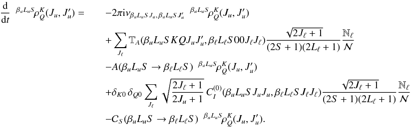 (59)As
expected, under the hypotheses of isotropic collisions and unpolarized lower term, transfer
processes due to inelastic collisions only contribute to the time evolution of the 0-rank
spherical statistical tensors of the upper term. Assuming that the colliding particles are
characterized by a Maxwellian velocity distribution, the collisional rates
(59)As
expected, under the hypotheses of isotropic collisions and unpolarized lower term, transfer
processes due to inelastic collisions only contribute to the time evolution of the 0-rank
spherical statistical tensors of the upper term. Assuming that the colliding particles are
characterized by a Maxwellian velocity distribution, the collisional rates
 and
and  can be related through the Milne-Einstein relation
![Mathematical equation: \begin{equation} C_S^{(0)}(\beta_{\ell} L_{\ell} S J_{\ell} J_{\ell}, \beta_u L_u S J_u J_u) = \frac{2J_{\ell} + 1}{2J_u +1} C_I^{(0)}(\beta_u L_u S J_u J_u, \beta_{\ell} L_{\ell} S J_{\ell} J_{\ell}) \, {\rm exp} \left[ \frac{E(\beta_u L_u S J_u) - E(\beta_{\ell} L_{\ell} S J_{\ell})}{K_B T} \right], \end{equation}](/articles/aa/full_html/2013/03/aa20511-12/aa20511-12-eq137.png) (60)where T is
the electron temperature. Using Eq. (38),
the fourth term on the righthand side of Eq. (59) can be written in the form
(60)where T is
the electron temperature. Using Eq. (38),
the fourth term on the righthand side of Eq. (59) can be written in the form
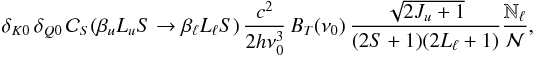 (61)where
BT(ν0) is the
Planck function in the Wien limit (consistently with the assumption of neglecting stimulated
emission) at temperature T, and where ν0 is the
Bohr frequency corresponding to the energy difference between the centers of gravity of the
two terms. (We neglect the frequency differences among the various components of the
multiplet in the exponential appearing in the Milne-Einstein relation.)
(61)where
BT(ν0) is the
Planck function in the Wien limit (consistently with the assumption of neglecting stimulated
emission) at temperature T, and where ν0 is the
Bohr frequency corresponding to the energy difference between the centers of gravity of the
two terms. (We neglect the frequency differences among the various components of the
multiplet in the exponential appearing in the Milne-Einstein relation.)
Taking the expression of  (see Eq.
(10.124) of LL04) into account and performing the sum over
Jℓ using Eq. (A.6), the second term on the righthand side of Eq. (59) is given by
(see Eq.
(10.124) of LL04) into account and performing the sum over
Jℓ using Eq. (A.6), the second term on the righthand side of Eq. (59) is given by
 (62)We recall that the
quantum theory of polarization described in LL04 is valid under the so-called flat spectrum
approximation (that is, the incident radiation field that produces optical pumping in the
atomic system must be flat over a frequency interval Δν larger than the
natural width of the atomic levels, and, when coherence between nondegenerate levels is
involved, Δν must then be larger than the corresponding Bohr frequency).
For this reason, it is sufficient to evaluate the radiation field tensor
(62)We recall that the
quantum theory of polarization described in LL04 is valid under the so-called flat spectrum
approximation (that is, the incident radiation field that produces optical pumping in the
atomic system must be flat over a frequency interval Δν larger than the
natural width of the atomic levels, and, when coherence between nondegenerate levels is
involved, Δν must then be larger than the corresponding Bohr frequency).
For this reason, it is sufficient to evaluate the radiation field tensor
 (see Eq.
(5.157) of LL04 for its definition) at a single frequency within the multiplet.
(see Eq.
(5.157) of LL04 for its definition) at a single frequency within the multiplet.
In stationary situations, recalling the relations among the Einstein coefficients
 (63)the spherical statistical
tensors of the upper term are given by
(63)the spherical statistical
tensors of the upper term are given by 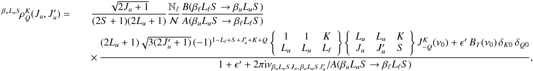 (64)where,
in analogy with the two-level atom case, we have introduced the quantity
(64)where,
in analogy with the two-level atom case, we have introduced the quantity
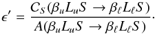 (65)It can be easily proven
that if S = 0, so that the upper and lower terms are composed by a single
fine-structure J-level, the expression of a two-level atom is recovered
(see Eq. (10.50) of LL04, with
(65)It can be easily proven
that if S = 0, so that the upper and lower terms are composed by a single
fine-structure J-level, the expression of a two-level atom is recovered
(see Eq. (10.50) of LL04, with  ).
).
Substituting Eq. (64) into Eq. (10.127) of
LL04, and introducing the frequency-integrated absorption coefficient of the
multiplet (66)and the absorption
profile of the multiplet (in the absence of magnetic fields, and for the case of a two-term
atom with unpolarized lower term)
(66)and the absorption
profile of the multiplet (in the absence of magnetic fields, and for the case of a two-term
atom with unpolarized lower term) 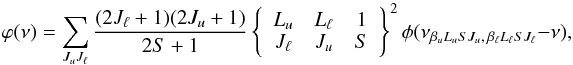 (67)where
φ(ν0 − ν) are Lorentzian
profiles centered at the frequencies of the various components of the multiplet, we find the
following expression of the emission coefficient in the four Stokes parameters:
(67)where
φ(ν0 − ν) are Lorentzian
profiles centered at the frequencies of the various components of the multiplet, we find the
following expression of the emission coefficient in the four Stokes parameters:
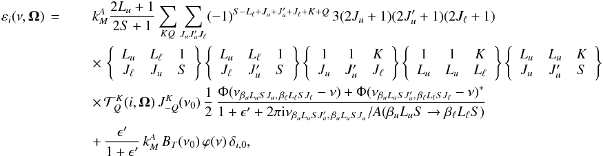 (68)with
i = 0, 1, 2, and 3, standing for Stokes I,
Q, U and V, respectively. Here,
ν and Ω are the frequency and propagation direction of the
emitted radiation, respectively,
(68)with
i = 0, 1, 2, and 3, standing for Stokes I,
Q, U and V, respectively. Here,
ν and Ω are the frequency and propagation direction of the
emitted radiation, respectively,  is the geometrical tensor
introduced by Landi Degl’Innocenti (1983), and
Φ(ν0 − ν) is the complex emission profile
is the geometrical tensor
introduced by Landi Degl’Innocenti (1983), and
Φ(ν0 − ν) is the complex emission profile
 (69)with
φ(ν0 − ν) a Lorentzian
profile and ψ(ν0 − ν) the
associated dispersion profile5. The last term on the
righthand side of Eq. (68) represents the
contribution to the emission coefficient coming from collisionally excited atoms. Since
collisions are assumed isotropic, this term only contributes to Stokes-I.
(69)with
φ(ν0 − ν) a Lorentzian
profile and ψ(ν0 − ν) the
associated dispersion profile5. The last term on the
righthand side of Eq. (68) represents the
contribution to the emission coefficient coming from collisionally excited atoms. Since
collisions are assumed isotropic, this term only contributes to Stokes-I.
As an example suitable to illustrating the sensitivity of the emergent scattering line
polarization to the studied collisional rates, we consider an isothermal slab of stellar
atmospheric plasma located at a given height above the surface of a solar-like star and
characterized by a given optical depth Δτ. Neglecting limb-darkening
effects, the radiation illuminating the slab from below is characterized by an anisotropy
factor  given by
 (70)
(70)
where α is half the angle subtended by the stellar disk, as seen from the slab. We solve the equations of the non-LTE problem described in this section for the case of a 2S − 2P transition, using the level energies and transition probabilities of the Mg ii h and k lines, and we calculate the fractional linear polarization of the radiation emerging at μ = cosθ = 0.1, with θ the angle formed by the local vertical (perpendicular to the slab) and the emission direction. The non-LTE radiative transfer problem is solved following the numerical methods described in Trujillo Bueno & Manso Sainz (1999).
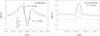 |
Fig. 1 Left panel: Q/I profile of the radiation emitted across a 2S − 2P transition (the level energies and transition probabilities are those of the Mg iih and k lines) as obtained for different values of the parameter ϵ′ (indicated in the plot). The arrows point to the wavelength positions of the two lines. Right panel: zoom of the line-core region of the 1/2−3/2 transition. We consider the radiation emitted at μ = 0.1 by a slab located 0.03 stellar radii above the surface, and with an optical depth (at the line-center frequency of the 1/2−1/2 transition) Δτ = 0.5. We solve the full non-LTE radiative transfer problem within the slab, the boundary condition being the stellar radiation illuminating the slab from below (limb-darkening effects are neglected). We consider a Doppler width of 26 mÅ, corresponding to a temperature of 104 K and a microturbulent velocity of 1 km s-1. We include the effect of an unpolarized continuum characterized by an opacity 108 times less than the line opacity at the line-center frequency of the 1/2−1/2 transition. The reference direction for positive Q is the parallel to the closest limb. |
Figure 1 shows the fractional linear polarization
Q/I pattern calculated for different
values of ϵ′, considering a slab located 0.03 stellar radii
above the surface (corresponding to about 2 × 10⁴ km in the solar case), and
characterized by an optical depth (at the line-center frequency of the
1/2−1/2 transition) Δτ = 0.5. We
assume a Doppler width of 26 mÅ, corresponding to a temperature of 104 K, and a
microturbulent velocity of 1 km s-1. The damping constant is consistently
calculated as 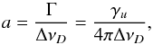 (71)with
 the inverse lifetime of the upper term (elastic collisions, hence their broadening effect,
are neglected). We include the contribution of an unpolarized continuum characterized by an
opacity
the inverse lifetime of the upper term (elastic collisions, hence their broadening effect,
are neglected). We include the contribution of an unpolarized continuum characterized by an
opacity  , with
 the line opacity at the
line-center frequency of the 1/2−1/2 transition. We
first note that in the slab model that we have considered (in which radiative transfer
effects are significant), the Q/I
profiles show the typical signatures of J-state interference, such as the
sign-reversal between the two lines, and the high polarization values in the far wings (see
Stenflo 1980, LL04; Belluzzi & Trujillo Bueno 2011). As can be observed, the
modification of the scattering line polarization pattern due to inelastic and superelastic
collisions (quenching effect) becomes appreciable only for rather high
values of the collisional rates (ϵ′ ≳ 10-2).
the line opacity at the
line-center frequency of the 1/2−1/2 transition. We
first note that in the slab model that we have considered (in which radiative transfer
effects are significant), the Q/I
profiles show the typical signatures of J-state interference, such as the
sign-reversal between the two lines, and the high polarization values in the far wings (see
Stenflo 1980, LL04; Belluzzi & Trujillo Bueno 2011). As can be observed, the
modification of the scattering line polarization pattern due to inelastic and superelastic
collisions (quenching effect) becomes appreciable only for rather high
values of the collisional rates (ϵ′ ≳ 10-2).
6. Conclusions
In this paper we have formally defined and investigated the transfer and relaxation rates due to isotropic inelastic and superelastic collisions that enter the statistical equilibrium equations for the atomic density matrix of a multiterm atom (i.e., a model atom accounting for quantum interference between magnetic sublevels pertaining either to the same J-level, or to different J-levels within the same term).
While the numerical values of the collisional rates for J-level populations are generally available (either from approximate theoretical expressions or from experimental data), the values of the collisional rates describing the transfer and relaxation of quantum coherence are in most cases unknown. In this work we focused our attention on the collisional rates for J-state interference (the physical aspect that cannot be accounted for with a multilevel model atom). Under the assumption that the interaction between the atom and the perturber is described by a dipolar operator, we derived suitable relations between such rates and the usual collisional rates for J-level populations. In particular, we showed that the collisional relaxation rate for J-state interference coincide with the relaxation rate for J-level populations and for interference between magnetic sublevels pertaining to the same J-level. We also observed that this rate does not depend on the particular J-level under consideration, so that it is sufficient to introduce a single collisional relaxation rate for the whole term. As a consistency proof of our derivations, we showed that the transfer and relaxation rates for J-level populations and for interference between pairs of magnetic sublevels pertaining to the same J-level reduce to those derived in Sect. 7.13 of LL04 for the multilevel atom case.
As an illustrative application, we considered an isothermal slab of given optical depth,
located at a given height above the surface of a solar-like star, and anisotropically
illuminated by its photospheric radiation field. The numerical solution of the full non-LTE
problem for the case of a two-term atom with unpolarized lower term shows that the
polarization of the radiation emerging from the slab at μ = 0.1 is
sensitive to the presence of isotropic inelastic and superelastic collisions only for values
of the parameter  on the order of 10-2 or larger. Such values are actually needed to produce an
appreciable variation in the Q/I
profiles of the emergent radiation.
on the order of 10-2 or larger. Such values are actually needed to produce an
appreciable variation in the Q/I
profiles of the emergent radiation.
We assume that there is no overlapping in energy among the various terms of the model atom under consideration.
The factor 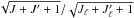 is introduced in order to get simpler relations between these rates and the usual
collisional rates connecting atomic populations. This factor reduces to the one introduced
in the multilevel atom case (see Eq. (7.87) of LL04) when interference between different
J-levels is neglected
(J = J′ and
).
is introduced in order to get simpler relations between these rates and the usual
collisional rates connecting atomic populations. This factor reduces to the one introduced
in the multilevel atom case (see Eq. (7.87) of LL04) when interference between different
J-levels is neglected
(J = J′ and
).
The sum appearing on the righthand side of Eq. (26) does not depend on the particular J-level of the lower term that is considered.
The sum appearing on the righthand side of Eq. (38) does not depend on the particular J-level of the upper term that is considered.
The equations derived here are valid in the atom rest frame. Nevertheless, under the assumption of complete redistribution on velocities (see Chapter 13 of LL04), the same equations can also be applied in the observer’s frame, with φ(ν0 − ν) and ψ(ν0 − ν) the Voigt profile and the Faraday-Voigt profile, respectively (provided that the atoms have a Maxwellian distribution of velocities).
Acknowledgments
Financial support by the Spanish Ministry of Science through projects AYA2010-18029 (Solar Magnetism and Astrophysical Spectropolarimetry) and CONSOLIDER INGENIO CSD2009-00038 (Molecular Astrophysics: The Herschel and Alma Era) is gratefully acknowledged.
References
- Belluzzi, L., & Trujillo Bueno, J. 2011, ApJ, 743, 3 [NASA ADS] [CrossRef] [Google Scholar]
- Bommier, V. 2009, in Solar Polarization 5, eds. S.V. Berdyugina, K. N. Nagendra, & R. Ramelli, ASP Conf. Ser., 405, 335 [Google Scholar]
- Landi Degl’Innocenti, E. 1983, Sol. Phys., 85, 1 [NASA ADS] [CrossRef] [Google Scholar]
- Landi Degl’Innocenti, E., & Landolfi, M. 2004, Polarization in Spectral Lines (Dordrecht: Kluwer) [Google Scholar]
- Seaton, M. J. 1962, in Atomic and Molecular Processes, ed. D.R. Bates (New York: Academic Press) [Google Scholar]
- Stenflo, J. O. 1980, A&A, 84, 68 [NASA ADS] [Google Scholar]
- Trujillo Bueno, J., & Manso Sainz, R. 1999, ApJ, 516, 436 [NASA ADS] [CrossRef] [Google Scholar]
- Van Regemorter, H. 1962, ApJ, 136, 906 [NASA ADS] [CrossRef] [Google Scholar]
Appendix A: Properties of 3-j and 6-j symbols and of rotation matrices
In this appendix we recall some useful properties and relations of 3-j and 6-j symbols, as well as of rotation matrices that are used in the derivation of the expressions presented in the paper. A proof of these properties can be found in Chap. 2 of LL04.
-
Symmetry properties of 3-j symbols: The 3-j symbols are invariant under cyclic permutations of their columns and are multiplied by (−1)a + b + c under noncyclic ones
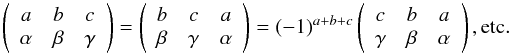 (A.1)The
3-j symbols are multiplied by
(−1)a + b + c
under sign inversion of the second row
(A.1)The
3-j symbols are multiplied by
(−1)a + b + c
under sign inversion of the second row 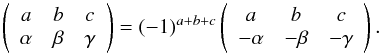 (A.2)
(A.2) -
Orthogonality relation of 3-j symbols
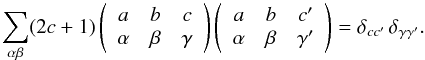 (A.3)
(A.3) -
Analytical expression of 3-j symbols for particular values of the arguments:
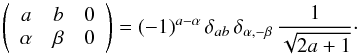 (A.4)
(A.4) -
Symmetry properties of 6-j symbols: The 6-j symbols are invariant under interchange of any two columns and under interchange of the upper and lower arguments in any two columns.
-
Sum rules of 6-j symbols:
-
Analytical expression of 6-j symbols for particular values of the arguments
 (A.7)
(A.7) -
Contraction of 3-j symbols:
 (A.8)
(A.8) -
Orthogonality relations of rotation matrices
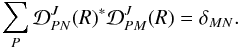 (A.9)
(A.9) -
Product of two rotation matrices:
 (A.10)
 (A.11)
All Figures
|
Fig. 1 Left panel: Q/I profile of the radiation emitted across a 2S − 2P transition (the level energies and transition probabilities are those of the Mg iih and k lines) as obtained for different values of the parameter ϵ′ (indicated in the plot). The arrows point to the wavelength positions of the two lines. Right panel: zoom of the line-core region of the 1/2−3/2 transition. We consider the radiation emitted at μ = 0.1 by a slab located 0.03 stellar radii above the surface, and with an optical depth (at the line-center frequency of the 1/2−1/2 transition) Δτ = 0.5. We solve the full non-LTE radiative transfer problem within the slab, the boundary condition being the stellar radiation illuminating the slab from below (limb-darkening effects are neglected). We consider a Doppler width of 26 mÅ, corresponding to a temperature of 104 K and a microturbulent velocity of 1 km s-1. We include the effect of an unpolarized continuum characterized by an opacity 108 times less than the line opacity at the line-center frequency of the 1/2−1/2 transition. The reference direction for positive Q is the parallel to the closest limb. |
| In the text | |
Current usage metrics show cumulative count of Article Views (full-text article views including HTML views, PDF and ePub downloads, according to the available data) and Abstracts Views on Vision4Press platform.
Data correspond to usage on the plateform after 2015. The current usage metrics is available 48-96 hours after online publication and is updated daily on week days.
Initial download of the metrics may take a while.