| Issue |
A&A
Volume 551, March 2013
|
|
|---|---|---|
| Article Number | A4 | |
| Number of page(s) | 15 | |
| Section | Astrophysical processes | |
| DOI | https://doi.org/10.1051/0004-6361/201220378 | |
| Published online | 07 February 2013 | |
Accretion disks around black holes in modified strong gravity
1 Instituto Argentino de Radioastronomía, Camino Gral Belgrano Km 40 C.C.5, 1984 Villa Elisa, Buenos Aires, Argentina
e-mail: This email address is being protected from spambots. You need JavaScript enabled to view it.
2 Facultad de Ciencias Astronómicas y Geofísicas, UNLP, Paseo del Bosque s/n CP, 1900 La Plata, Buenos Aires, Argentina
e-mail: This email address is being protected from spambots. You need JavaScript enabled to view it.
3 Departamento de Física Teórica, Instituto de Física, Universidade do Estado do Rio de Janeiro, Rua São Francisco Xavier 524, Maracanã, Rio de Janeiro, CEP: 20550-900, Brasil
e-mail: This email address is being protected from spambots. You need JavaScript enabled to view it.
Received: 13 September 2012
Accepted: 18 November 2012
Abstract
Context. Stellar-mass black holes offer what is perhaps the best scenario to test theories of gravity in the strong-field regime. In particular, f(R) theories, which have been widely discus in a cosmological context, can be constrained through realistic astrophysical models of phenomena around black holes.
Aims. We aim at building radiative models of thin accretion disks for both Schwarzschild and Kerr black holes in f(R) gravity.
Methods. We study particle motion in f(R)-Schwarzschild and Kerr space-times.
Results. We present the spectral energy distribution of the accretion disk around constant Ricci scalar f(R) black holes, and constrain specific f(R) prescriptions using features of these systems.
Conclusions. A precise determination of both the spin and accretion rate onto black holes along with X-ray observations of their thermal spectrum might allow to identify deviations of gravity from general relativity. We use recent data on the high-mass X-ray binary Cygnus X-1 to restrict the values of the parameters of a class of f(R) models.
Key words: black hole physics / accretion, accretion disks / gravitation
© ESO, 2013
1. Introduction
General relativity (GR) is consistent, in some cases with good precision, with observational results (see for instance Will 2006). However, an energy momentum tensor representing exotic matter (loosely called “dark energy”, e.g. Li et al. 2011) must be introduced in the right hand side of Einstein’s equations to fit the currently available data when these are interpreted in the framework of the standard cosmological model (based on GR). Dark energy can be modelled by a cosmological constant, or by a scalar field with an equation of state given by p = ωDEρ, where ωDE < −1/3 (Biswas et al. 2010a,b). None of these descriptions is free of problems, since the energy density associated with the cosmological constant that is inferred from astronomical observations is approximately 120 orders of magnitude lower than the value predicted by field theory (e.g. Weinberg 1989; Capozziello & Faraoni 2010), whereas the scalar field has features that are at odds with the scalar fields of particle physics (Sotiriou & Faraoni 2010).
A different approach to explain the cosmological data is to modify the field equations of the gravitational field, in such a way that the ensuing theory differs from Einstein’s in the low-curvature regime. Since there is no a priori fundamental reason to restrict the gravitational Lagrangian to a linear function of the Ricci scalar R (see for instance Magnano et al. 1987), more general theories can be formulated using nonlinear functions of this scalar. The so-called f(R) theories (e.g. Capozziello & Faraoni 2010) were first used to mimic the inferred accelerated expansion of the universe by Capoziello (2002). Currently there is in the literature a handful of f(R)-models in agreement with available data (De Felice & Tsujikawa 2010).
Although the present revival of f(R) theories is mainly due to their use in the description of phenomena that take place for low values of the Riemann curvature, these theories have also been applied to gravity in the opposite regime. As there is no direct evidence of the behaviour of the gravitational field for very large values of the curvature, the early universe and compact objects offer the possibility to find deviations from GR. Among the studies in modified gravity in the strong regime, we can mention the successful inflationary model based on the R + αR2 theory (Starobinsky 1980), and the related studies of reheating (Motohashi & Nishizawa 2012) and particle production (Arbuzova et al. 2012) in the early universe. Also of importance is the treatment of neutron stars (Cooney et al. 2010) and black hole solutions.
Different aspects of black hole physics in f(R) theories have been discussed in the literature by Psaltis et al. (2008a), Hendi & Momeni (2011), Myung (2011), Myung et al. (2011), Moon et al. (2011a,b), Hendi et al. (2012), and Habib Mazharimousavi et al. (2012). Static and spherically symmetric black hole solutions were obtained via perturbation theory by de la Cruz-Dombriz et al. (2009), whereas black holes with these symmetries have been studied by means of a near-horizon analysis by Perez Bergliaffa & De Oliveira (2011). Finally, f(R)-Kerr-Newman black holes solutions with constant Ricci scalar have been recently studied by Cembranos and collaborators (Cembranos et al. 2011).
From an astrophysical point of view, thin accretion for the Schwarzschild space-time in f(R)-gravity has been discussed by Pun et al. (2008), without including the expected spectra of concrete astrophysical black holes or any comparison with observational data.
In the present work we investigate the existence of stable circular orbits in Schwarzschild and Kerr f(R) space-times with constant Ricci scalar and analyze the main features of accretion disks around these black holes. In particular, we present temperature and spectral energy distributions for Page-Thorne disks, and compare the results with those obtained using the standard Shakura-Sunyaev model.
The paper is organized as follows. In Sect. 2 we provide a brief review of f(R) theories of gravity. Circular orbits in both Schwarzschild and Kerr f(R) space-times with constant Ricci scalar are studied in Sect. 3. Section 4 is devoted to the calculation of the properties of accretion disks in these space-times. Consequences for some specific prescriptions for the function f are discussed in Sect. 5. We close with some considerations on the potential of astronomical observations to test the strong-field regime of gravity.
2. f(R) gravity
In f(R) gravity, the Lagrangian of the Hilbert-Einstein action, given by: ![Mathematical equation: \begin{equation} S[g] = \frac{c^{3}}{16\pi G}\int R \sqrt{-g}\; {\rm d}^{4}x, \end{equation}](/articles/aa/full_html/2013/03/aa20378-12/aa20378-12-eq7.png) (1)is generalized to:
(1)is generalized to: ![Mathematical equation: \begin{equation} \label{lagrafr} S[g] = \frac{c^{3}}{16\pi G}\int \left(R +f(R)\right) \sqrt{-g}\; {\rm d}^{4}x, \end{equation}](/articles/aa/full_html/2013/03/aa20378-12/aa20378-12-eq8.png) (2)where g is the determinant of the metric tensor, and f(R) is an arbitrary function of the Ricci scalar. In the metric formalism the field equations are obtained varying Eq. (2) with respect to the metric:
(2)where g is the determinant of the metric tensor, and f(R) is an arbitrary function of the Ricci scalar. In the metric formalism the field equations are obtained varying Eq. (2) with respect to the metric: 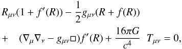 (3)where Rμν is the Ricci Tensor, □ ≡ ∇β∇β, f′(R) = df(R)/dR, and the energy momentum tensor is defined by:
 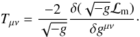 (4)Here, ℒm stands for the matter Lagrangian.
Equations (3) are a system of fourth-order nonlinear equations for the metric tensor gμν. An important difference between them and the Einstein field equations is that in f(R) theories the Ricci scalar R and the trace T of the energy momentum tensor are differentially linked, as can be seen by taking the trace of Eq. (3), which yields: 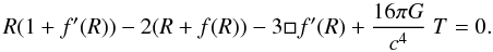 (5)Hence, depending on the form of the function f, there may be solutions with traceless energy-momentum tensor and nonzero Ricci scalar. This is precisely the case of black hole space-times in the absence of a matter source.
Notice that in the case of constant Ricci scalar R0 without matter sources, Eqs. (3) can be re-written as:
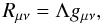 where:
  (6)and, by Eq.(5):
  (7)Hence, in this case, any f(R) theory is formally, but not physically, equivalent to GR with a cosmological constant given by Eq. (6)1.
We shall investigate the existence of stable circular orbits in Schwarzschild and Kerr f(R) space-times with constant Ricci scalar in the next section.
3. Circular orbits around a black hole in f(R)
3.1. f(R)-Schwarzschild space-time
The Schwarzschild space-time metric in f(R) theories with constant Ricci scalar R0 takes the form (Cembranos et al. 2011): ![Mathematical equation: \begin{eqnarray} \label{g-Sc} {\rm d}s^{2}& = &-\left[\left(c^{2}-\frac{2GM}{r}\right)-\frac{c^{2}R_{{0}}}{12}r^{2}\right]\\ \nonumber {\rm d}t^{2} & + & \frac{{\rm d}r^{2}}{\left[\left(1-\frac{2MG}{c^{2}r}\right)-\frac{R_{{0}}}{12}r^{2}\right]} + r^{2} \left({\rm d}\theta^{2}+\sin^{2}\theta {\rm d}\phi^{2}\right), \end{eqnarray}](/articles/aa/full_html/2013/03/aa20378-12/aa20378-12-eq24.png) (8)where R0, given by Eq. (7), can take, in principle, any real value. Since we are looking for space-time metrics that may represent astrophysical black holes, we shall select those values of R0 that lead to acceptable solutions.
(8)where R0, given by Eq. (7), can take, in principle, any real value. Since we are looking for space-time metrics that may represent astrophysical black holes, we shall select those values of R0 that lead to acceptable solutions.
The radius r0 of the horizon follows from the condition g00(r0) = 0. From Eq. (8), the values of r corresponding to the event horizon satisfy:  (9)In terms of the following adimensional quantities:
  where rg = GM/c2, this equation takes the form:
  (12)We show in Fig. 1 the Ricci scalar as a function of the radial coordinate of the event horizon. We see that for R0 ∈ (0,4/9) there is an inner black hole event horizon and an outer cosmological horizon, whereas for R0 ≤ 0 there is only one black hole event horizon. The event and cosmological horizons collapse for R0 = 4/9 and for larger values of the Ricci scalar naked singularities occur and hence, no black holes are possible2. We shall, then, restrict ourselves to the study of trajectories for R0 ∈ ( − ∞,4/9] .
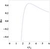 |
Fig. 1 Ricci scalar as a function of the radial coordinate of the event horizon in f(R)-Schwarzschild space-time. |
3.1.1. Equations of motion and effective potential in f(R)-Schwarzschild space-time
The geodesic equations in the metric given in Eq. (8) can be obtained by means of the Euler-Lagrange equations using the Lagrangian: ![Mathematical equation: \begin{eqnarray} \label{lagr-sc} L & = & - \left[\left(c^{2}-\frac{2GM}{r}\right)-\frac{c^{2}R_{{0}}}{12}r^{2}\right] \dot{t}^{2}\\ \nonumber & &+ \frac{1}{\left[\left(1-\frac{2GM}{c^{2}r}\right)-\frac{R_{{0}}}{12}r^{2}\right]} \dot{r}^{2} +r^{2}\left(\dot{\theta}^{2}+{\sin \theta}^{2} \dot{\phi}^{2}\right), \end{eqnarray}](/articles/aa/full_html/2013/03/aa20378-12/aa20378-12-eq36.png) (13)where ẋμ ≡ dxμ/dσ, and σ is an affine parameter along the geodesic xμ(σ). The resulting geodesic equations for t and φ are (setting θ = π/2):
(13)where ẋμ ≡ dxμ/dσ, and σ is an affine parameter along the geodesic xμ(σ). The resulting geodesic equations for t and φ are (setting θ = π/2): ![Mathematical equation: \begin{eqnarray} \left[\left(1-\frac{2GM}{c^{2}r}\right)-\frac{R_{{0}}}{12}r^{2}\right] \dot{t} & = & k,\label{et}\\ r^{2} \dot{\phi} &=& h\label{ephi}, \end{eqnarray}](/articles/aa/full_html/2013/03/aa20378-12/aa20378-12-eq43.png) where k and h are constants. An equation for r that is simpler than the one obtained from the Lagrangian follows from the modulus of the 4-momentum p, given by gμνxμxν = ϵ2, where ϵ2 = c2 for massive particles, and ϵ2 = 0 for photons. It takes the form:
where k and h are constants. An equation for r that is simpler than the one obtained from the Lagrangian follows from the modulus of the 4-momentum p, given by gμνxμxν = ϵ2, where ϵ2 = c2 for massive particles, and ϵ2 = 0 for photons. It takes the form: ![Mathematical equation: \begin{eqnarray} \label{er} &&- \left[\left(c^{2}-\frac{2GM}{r}\right)-\frac{c^{2}R_{{0}}}{12}r^{2}\right] \dot{t}^{2}\nonumber\\ &&\qquad\quad + \frac{\dot{r}^{2}}{\left[\left(1-\frac{2GM}{c^{2}r}\right)-\frac{R_{{0}}}{12}r^{2}\right]} + r^{2} \dot{\phi}^{2} = \epsilon^{2}, \end{eqnarray}](/articles/aa/full_html/2013/03/aa20378-12/aa20378-12-eq50.png) (16)with ṫ and
(16)with ṫ and  given by Eqs. (14) and (15), respectively. The set of Eqs. (14), (15), and (16) completely determine the motion of a particle in the f(R)-Schwarzschild space-time.
3.1.2. Trajectories of massive particles
Equations (14), (15), and (16) can be used to obtain the so-called energy equation (e.g. Hobson et al. 2006): ![Mathematical equation: \begin{eqnarray} \label{energy1} &&\dot{r}^{2}+\frac{h^{2}}{r^{2}} \left[\left(1-\frac{2GM}{c^{2}r}\right)-\frac{R_{{0}}}{12}r^{2}\right]\nonumber\\ &&\qquad\quad+\left(-\frac{2GM}{r}-\frac{c^2R_{{0}}}{12}r^{2}\right) = c^{2}(k^{2}-1). \end{eqnarray}](/articles/aa/full_html/2013/03/aa20378-12/aa20378-12-eq53.png) (17)The constant k is defined as k = E/m0c2, where E represents the total energy of the particle in its orbit, and m0c2 its rest mass energy. The constant h stands for the angular momentum of the particle per unit mass. From Eq. (17) we can identify the effective potential per unit mass as:
(17)The constant k is defined as k = E/m0c2, where E represents the total energy of the particle in its orbit, and m0c2 its rest mass energy. The constant h stands for the angular momentum of the particle per unit mass. From Eq. (17) we can identify the effective potential per unit mass as:  (18)The extrema of the effective potential are obtained by looking for the roots of the derivative of the latter equation with respect to the radial coordinate. In terms of x, R0, and the adimensional angular momentum per unit mass of the particle h = h(crg)-1, this reads:
  (19)The derivative of Eq. (19) with respect to x gives:
 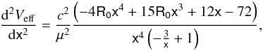 (20)where we have replaced h by (Harko et al. 2009):
 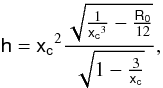 (21)where xc corresponds to the radius of a circular orbit. We have performed the numerical calculation of the extrema of the effective potential for different values of R0.
Location of the event and cosmological horizon, and of the innermost and outermost stable circular orbits for R0 > 0 in f(R)-Schwarzschild space-time.
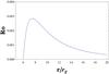 |
Fig. 2 Function given by Eq. (23). The absolute maximum corresponds to x = 15/2 and R0 = 2.85 × 10⁻³. |
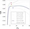 |
Fig. 3 Effective potential for different values of R0 > 0 and h in f(R)-Schwarzschild space-time. The dots indicate the location of the innermost stable circular orbit. |
For R0 > 0, as shown by Stuchlík et al. (1999) and Rezzolla et al. (2003) in Schwarzschild-de Sitter space-time, stable circular orbits exist for values of the specific angular momentum that satisfy:  (22)where hisco and hosco stand for the local minimum and local maximum of the specific angular momentum at the inner and outer marginally stable radii. From Eq. (20) we see that the existence and location of the circular orbits depend on the Ricci scalar R0. By equating Eq. (19) to zero and isolating R0, we obtain the Ricci scalar as a function of the radial coordinate of the circular orbits:
  (23)In Fig. 2 we show the plot of the latter equation. We see that there is an upper limit for the Ricci scalar, R0 = 2.85 × 10⁻³, for which circular orbits are possible. In Fig. 3 we plot the effective potential as a function of the radial coordinate. The dots indicate the location of the innermost stable circular orbits. The corresponding values of the event and cosmological horizons, radii of the innermost and outermost stable circular orbits, for six different values of R0 ∈ (0,2.85 × 10-3) are shown in Table 1. We see that for increasing values of the Ricci scalar the event horizon becomes larger than in Schwarzschild space-time in GR as well as the location of the innermost stable circular orbit.
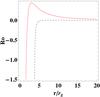 |
Fig. 4 Ricci scalar as a function of the radial coordinate of the event horizon (line) and of the Ricci scalar as a function of the radial coordinate of the innermost stable circular orbits (dashed line) for R0 ∈ [ − 1.5,0.45] in f(R)-Schwarzschild space-time. |
The extrema of the effective potential for R0 < 0 are all located outside the event horizon, as shown in Fig. 4. The value of the radial coordinate for the event horizon is less than 2 (i.e. smaller than for Schwarzschild black holes in GR). The location of the innermost stable circular orbit is closer to the horizon than that of the Schwarzschild solution in Einstein’s gravity. The limit R0 → − ∞ in Eq. (20) yields:  (24)The plot of the effective potential corresponding to the values of the parameters of Table 2 is shown in Fig. 5.
Location of the event horizon, and of the innermost stable circular orbit for R0 < 0 in f(R)-Schwarzschild space-time.
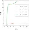 |
Fig. 5 Effective potential for different values of R0 < 0 and h in f(R)-Schwarzschild space-time. The dots indicate the location of the innermost stable circular orbit. |
3.2. Kerr space-time in f(R) theories
The axisymmetric, stationary and constant Ricci scalar geometry that describes a black hole with mass, electric charge and angular momentum was found by Carter (1973), and was used to study f(R) black holes by Cembranos et al. (2011). The form of the metric is the following: ![Mathematical equation: \begin{eqnarray} \label{kerr-ftot} {\rm d}s^{2}& = &\frac{\rho^2}{\Delta_{\rm r}} {\rm d}r^{2}+\frac{\rho^2}{\Delta_{\rm \theta}} {{\rm d}\theta}^{2}\\ \nonumber & &+ \frac{\Delta_{\rm \theta}\: {\sin^{2}{\theta}}}{\rho^{2}}\left[a\:\frac{c\:{\rm d}t}{\Xi}-\left(r^{2}+a^{2}\right)\frac{{\rm d}\phi}{\Xi}\right]^{2}\\ \nonumber &&-\frac{\Delta_{\rm r}}{\rho^{2}}\left(\frac{c\:{\rm d}t}{\Xi}-a\:{\sin^{2}{\theta}}\frac{{\rm d}\phi}{\Xi}\right)^{2}, \end{eqnarray}](/articles/aa/full_html/2013/03/aa20378-12/aa20378-12-eq123.png) (25)where:
(25)where:  Here M and a denote the mass and angular momentum per unit mass of the black hole, respectively, and R0 is given by Eq.(7).
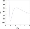 |
Fig. 6 Ricci scalar as a function of the radial coordinate of the event horizon for R0 ∈ [ − 0.3,1] and a = 0.99 in f(R)-Kerr space-time. |
Because of the constancy of pt and pφ along the trajectories, and of the reflection-symmetry of the metric through the equatorial plane, the orbit of any particle with initial condition pθ = 0 will remain in the plane π/2, where the metric has the form: ![Mathematical equation: \begin{eqnarray} \label{Kr-metric} {\rm d}s^{2} & = & -\frac{c^2}{r^2 \Xi^2} \left(\Delta_{r}-a^{2}\right){\rm d}t^{2}+\frac{r^{2}}{\Delta_{r}} {\rm d}r^{2}\\ \nonumber &&-\frac{2ac}{r^{2}\Xi^{2}} \left(r^{2}+a^{2}-\Delta_{r}\right) {\rm d}t {\rm d}\phi \\ \nonumber &&+ \frac{d\phi^{2}}{r^{2}\Xi^{2}} \left[\left(r^{2}+a^{2}\right)^{2}-\Delta_{r} a^{2}\right]. \end{eqnarray}](/articles/aa/full_html/2013/03/aa20378-12/aa20378-12-eq133.png) (30)Here,
(30)Here,  If R0 → 0, Eq. (30) represents the Kerr space-time metric in GR as expected.
The equation that yields the position of the event horizon is obtained by setting 1/grr = 0:  (33)In terms of x, R0, and a ≡ a(rg)-1, this equation takes the form:
 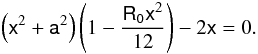 (34)In Fig. 6 we plotted the Ricci scalar as a function of the radial coordinate of the event horizon for R0 ∈ [−0.3,1] and a = 0.99 (i.e. a nearly maximally rotating black hole, such as Cygnus X1, Gou et al. 2011). If R0 ∈ (0,0.6] , there are 3 event horizons: the inner and outer horizons of the black hole and a cosmological horizon; for R0 > 0.6 there is a cosmological horizon that becomes smaller for larger values of R0. If R0 ∈ (−0.13,0) there are 2 event horizons. For R0 ≤ −0.13 naked singularities occur. In the following we shall analyse the existence of stable circular orbits for R0 ∈ (−0.13,0.6] .
3.2.1. Equations of motion and effective potential in f(R)-Kerr space-time
In order to obtain an expression for the effective potential, we make use of the invariant length of the 4-momentum p: 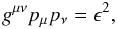 (35)where ϵ2 = c2 for massive particles and ϵ2 = 0 for photons. Since we are only interested in trajectories on the equatorial plane, we set pθ = 0, and Eq. (35) gives:
  (36)where:
 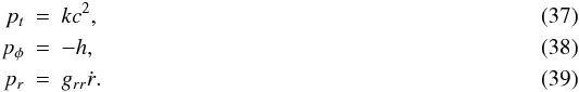 Substituing Eqs. (37), (38), and (39) into (36), the equation for ṙ2 takes the form:
 ![Mathematical equation: \begin{equation} {\dot{r}}^{2} = g^{rr} \left[\epsilon^{2}-g^{tt} \left(kc^{2}\right)^{2}+ 2 g^{t\phi} hkc^{2}-g^{\phi \phi} h^{2}\right]. \end{equation}](/articles/aa/full_html/2013/03/aa20378-12/aa20378-12-eq152.png) (40)The contravariant components of the space-time metric given by Eq. (30) are:
(40)The contravariant components of the space-time metric given by Eq. (30) are: ![Mathematical equation: \begin{eqnarray} g^{tt} & = & \frac{\Xi^{2}}{\Delta_{r} \;c^2 r^{2}}\left[\left(r^{2}+a^{2}\right)^{2}-\Delta_{r}a^{2}\right], \label{gc1} \\ g^{rr} & = & -\frac{\Delta_{r}}{r^{2}}, \label{gc2} \\ g^{t \phi} & = & \frac{\Xi^{2}}{c \Delta_{r} \;r^{2}} a \left(r^{2}+a^{2}-\Delta_{r}\right), \label{gc3} \\ g^{\phi \phi} & = & -\frac{\Xi^{2}}{\Delta_{r}\; r^{2}} \left(\Delta_{r}-a^{2}\right).\label{gc4} \end{eqnarray}](/articles/aa/full_html/2013/03/aa20378-12/aa20378-12-eq153.png) Hence, the energy equation for a massive particle is given by:
Hence, the energy equation for a massive particle is given by:  (45)where the effective potential is:
 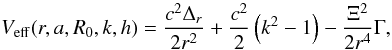 (46)and:
 ![Mathematical equation: \begin{equation} \Gamma \equiv \left[\left(r^{2}+a^{2}\right)ck-a h\right]^{2}-\Delta_{r}\left(ack-h\right)^{2}. \end{equation}](/articles/aa/full_html/2013/03/aa20378-12/aa20378-12-eq156.png) (47)
(47)
3.2.2. Equatorial circular orbits of massive particles
If a massive particle is moving in a circular orbit of radius risco, the value of the effective potential at any point of the orbit satisfies the equation:  (48)so,
  (49)For a stable orbit, the equation:
  (50)must also be satisfied. As shown in Sect. 3.2, there are black holes if R0 ∈ ( − 0.13,0.6] .
Radii of event horizons and circular orbits for a f(R)-Kerr black hole of angular momentum a = 0.99, for some values of R0 < 0.
Numerical calculations of the radius of the innermost stable circular orbit for several values of R0 < 0, with a = 0.99, show that the stable circular orbits lay outside the event horizon (see Table 3). Notice that as the value of the scalar decreases, the radius of the innermost stable circular orbit becomes smaller. The radius of the innermost stable circular orbit in Kerr space-time in GR (risco = 1.4545rg, in the prograde case) is always larger than in f(R)-Kerr. In Fig. 7, the effective potential that correspond to the values of Table 3 are shown.
Location of the event and cosmological horizon, and of the innermost and outermost stable circular orbits for R0 > 0 and a = 0.99 in f(R)-Kerr space-time.
We follow Stuchlík & Slaný (2004) to study the existence of stable circular orbits for R0 ∈ (0,0.6] . The specific angular momentum of a massive particle in a co-rotating circular orbit yields (Stuchlík & Slaný 2004): ![Mathematical equation: \begin{equation} \label{hpos} \mathsf{h} = -\frac{2\mathsf{a}+\mathsf{a}\mathsf{x_c}\left(\mathsf{x_c}^{2}+\mathsf{a}^{2}\right)\frac{\mathsf{R_{0}}}{12}-\mathsf{x_c}\left(\mathsf{x_c}^{2}+\mathsf{a}^{2}\right)\left(\frac{1}{\mathsf{x_c}^{3}}-\frac{\mathsf{R_{0}}}{12}\right)^{1/2}}{\mathsf{x_c}\left[1-\frac{3}{\mathsf{x_c}}-\frac{\mathsf{a}^{2}R_{0}}{12}+2\mathsf{a}\left(\frac{1}{\mathsf{x_c}^{3}}-\frac{\mathsf{R_0}}{12}\right)^{1/2}\right]^{1/2}}\cdot \end{equation}](/articles/aa/full_html/2013/03/aa20378-12/aa20378-12-eq204.png) (51)We see from the latter equation that circular orbits must satisfy the following two conditions:
(51)We see from the latter equation that circular orbits must satisfy the following two conditions:  (52)which is the same for f(R)-Schwarzschild space-time with positive Ricci scalar, and:
  (53)The minimum and maximum of Eq. (51) give the values of the specific angular momentum that correspond to the innermost and outermost stable circular orbit respectively, once the angular momentum a of the black hole and R0 are fixed. We show in Table 4 the values of such radii for different values of R0, and a = 0.99, and in Fig. 8 the corresponding plot of the effective potential. As expected, the radius of inner circular orbit is larger than in Kerr space-time in GR. We also found, by equating to zero the derivative of Eq. (51), that stable circular orbits only exist if R0 ∈ (0,1.45 × 10-1).
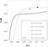 |
Fig. 7 Effective potential as a function of the radial coordinate (R0 < 0, a = 0.99), in f(R)-Kerr space-time. The dots indicate the location of the innermost stable circular orbit. |
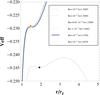 |
Fig. 8 Effective potential as a function of the radial coordinate (R0 > 0, a = 0.99), in f(R)-Kerr space-time. The dots indicate the location of the innermost stable circular orbit. |
The analysis of the circular orbits presented in this section will be applied next to the construction of accretion disks around black holes.
4. Accretion disks in strong gravity
4.1. Standard disk model in general relativity
The first realistic model of accretion disks around black holes was formulated by Shakura & Sunyaev (1973). They considered that the matter rotating in circular Keplerian orbits around the compact object loses angular momentum because of the friction between adjacent layers and spirals inwards. In the process gravitational energy is released, the kinetic energy of the plasma increases and the disk heats up, emitting thermal energy.
Novikov, Thorne, and Page (Novikov & Thorne 1973; Page & Thorne 1974) made a relativistic analysis of the structure of an accretion disk around a black hole. They assumed the background space-time geometry to be stationary, axially-symmetric, asymptotically flat, and reflection-symmetric with respect to the equatorial plane. They also postulated that the central plane of the disk coincides with the equatorial plane of the black hole. This assumption entails that the metric coefficients gtt, gtφ, grr, gθθ, and gφφ depend only on the radial coordinate r.
The disk is supposed to be in a quasi-steady state (Novikov & Thorne 1973), so any relevant quantity (for example the density or the temperature of the gas) is averaged over 2π, a proper radial distance of order 2H3, and the time interval Δt that the gas takes to move inward a distance 2H. During Δt, the changes in the space-time geometry are negligible.
Particles move in the equatorial plane in nearly geodesic orbits; consequently, the gravitational forces exerted by the black hole completely dominate over the radial accelerations due to pressure gradients.
The expression of the energy flux for a relativistic accretion disk takes the form (Novikov & Thorne 1973; Page & Thorne 1974):  (54)where
  stands for the mass accretion rate, Ω for the angular velocity and
  and
and  represent the specific energy and angular momentum, respectively. The lower limit of the integral risco corresponds to the location of the innermost stable circular orbit.
The angular velocity Ω, the specific energy , and the specific angular momentum of the particles moving in circular orbits are given by (Harko et al. 2009):  Equations (56), and (57) can be derived by writing the effective potential Veff(r) in terms of the metric coefficients and solving for and the equations Veff(r) = 0 and Veff,r(r) = 0. The formula for the angular velocity Ω = dφ/dt is obtained by substituing , and into the geodesic equations dt/dτ and dφ/dτ (Harko et al. 2009).
In the next subsections we calculate the energy flux, temperature and luminosity of an accretion disk around a Schwarzschild and a Kerr black hole in GR and f(R) gravity with constant Ricci scalar, adopting the following values for the relevant parameters: M = 14.8 M⊙, Ṁ = 0.472 × 10¹⁹ g s-1, and a = 0.99, which are the best estimates available for the well-known galactic black hole Cygnus-X1 (Orosz et al. 2011; Gou et al. 2011).
4.1.1. Relativistic accretion disk around Schwarzschild and Kerr black holes
In order to obtain an expression of the energy flux and temperature of the disk, for the Schwarzschild black hole, we calculate the angular velocity Ω, the specific energy and angular momentum of the particles in the disk, using the metric (Schwarzschild 1916): 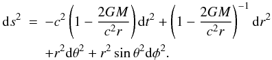 (58)From Eqs. (55)–(57) we get:
 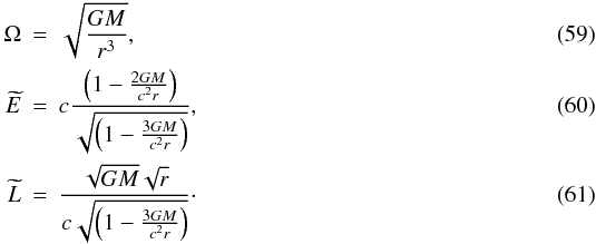 By replacing these equations in Eq. (54), we obtain:
 ![Mathematical equation: \begin{eqnarray} \label{fluxsch} Q(\mathsf{x})& =& \frac{3 \dot{M_{0}} c^{6}}{8 \pi \mathsf{x}^{7/2}} \frac{1}{\left(GM\right)^{2}}\left(1-\frac{3}{\mathsf{x}}\right)^{-1} \\ \nonumber & &\times\left[\sqrt{\mathsf{x}}+\sqrt{3}\tanh^{-1}\sqrt{\frac{\mathsf{x}}{3}}\;\right]^{\mathsf x}_{\mathsf{x_{{\rm isco}}}}, \end{eqnarray}](/articles/aa/full_html/2013/03/aa20378-12/aa20378-12-eq235.png) (62)where xisco = 6rg is the location of the innermost stable circular orbit in Schwarzschild space-time.
(62)where xisco = 6rg is the location of the innermost stable circular orbit in Schwarzschild space-time.
By means of Stefan-Bolzmann’s law, 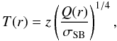 (63)(where z stands for the correction due to the gravitational redshift), the temperature of the disk can be obtained as a function of the radial coordinate r.
In Figs. 9 and 10 we plot the energy flux and the temperature as a function of the radial coordinate for a Schwarzschild black hole in both Keplerian and relativistic accretion disk models. We see that GR effects introduce a decrease of the peak of the energy flux by a factor ≈ 2, and that the temperature distribution is also diminished.
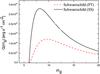 |
Fig. 9 Energy flux as a function of the radial coordinate of an accretion disk around a Schwarzschild black hole in Shakura-Sunyaev (SS) and Page-Thorne (PT) models, respectely. |
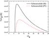 |
Fig. 10 Temperature as a function of the radial coordinate of an accretion disk around a Schwarzschild black hole in SS and PT models, respectively. |
The Kerr space-time metric (Kerr 1963) in Boyer-Lindquist coordinates for θ = π/2 is: ![Mathematical equation: \begin{eqnarray} \label{K-metric} {\rm d}s^{2} &=& -\frac{c^2}{r^2} \left(\Delta_{r}-a^{2}\right)dt^{2}+\frac{r^{2}}{\Delta_{r}} {\rm d}r^{2}\\ \nonumber && -\frac{2ac}{r^{2}} \left(r^{2}+a^{2}-\Delta_{r}\right) {\rm d}t {\rm d}\phi \\ \nonumber & &+ \frac{d\phi^{2}}{r^{2}} \left[\left(r^{2}+a^{2}\right)^{2}-\Delta_{r} a^{2}\right], \end{eqnarray}](/articles/aa/full_html/2013/03/aa20378-12/aa20378-12-eq241.png) (64)where:
(64)where: 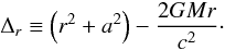 (65)The expression of the energy flux now becomes:
  (66)where:
 ![Mathematical equation: \begin{eqnarray} &&\left(\widetilde{E}-\Omega\widetilde{L}\right) \widetilde{L,_{r}} = - \frac{c}{2}\frac{\left[\left(p_{1}+p_{2}\right)\:p_{3}\right]}{p_{4}}, \\ &&- \frac{\dot{M_{0}}}{4\pi \sqrt{-g}}\frac{\Omega,_{r}}{\left(\widetilde{E}-\Omega\widetilde{L}\right)^{2}} = \frac{3\dot{M_0}}{8\pi}\frac{c^{2}}{\mu^{2}}\frac{p_{5}}{\left(p_{1}+p_{2}\right)^{2}}, \end{eqnarray}](/articles/aa/full_html/2013/03/aa20378-12/aa20378-12-eq244.png) and the coefficients pi are given by:
and the coefficients pi are given by: 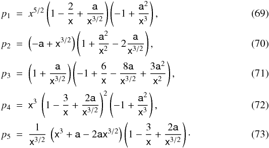 Here x = r/rg is an adimensional radial coordinate, and a = a/rg is the angular momentum of the black hole in adimensional units.
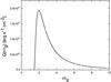 |
Fig. 11 Energy flux as function of the radial coordinate for an accretion disk around a Kerr black hole of angular momentum a = 0.99 in the PT model. |
In Figs. 11 and 12 we show the plots of the energy flux and temperature of an accretion disk around a Kerr black hole of angular momentum a = 0.99, whose innermost stable circular orbit is at risco = 1.4545rg. In Fig. 13 we show the luminosity of relativistic accretion disks around both Schwarzschild and Kerr black holes. For comparison, we also present the Schwarzschild/Shakura-Sunyaev luminosity.
The values of the maximum temperature, luminosity, and the energy of the peak of the emission for all these models are shown in Table 5. As expected, the highest luminosity corresponds to a prograding accretion disk around a Kerr black hole. Since the last stable circular orbit is located closer to the black hole than in Schwarzschild space-time, thermal radiation is emitted at higher energies.
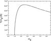 |
Fig. 12 Temperature as function of the radial coordinate of an accretion disk around a Kerr black hole of angular momentum a = 0.99 in the PT model. |
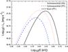 |
Fig. 13 Luminosity as function of the energy for a relativistic accretion disk around a Schwarzschild and a Kerr black hole (a = 0.99). We also plot the luminosity as a function of the energy of an accretion disk around a Schwarzschild black hole that corresponds to the SS model. |
Values of the energy of the peak of the emission, the maximum temperature, and luminosity of an accretion disk around Schwarzschild and Kerr black holes (a = 0.99) in the SS and PT models.
4.2. f(R)-gravity
4.2.1. f(R)-Schwarzschild black holes
The energy flux of an accretion disk around a f(R)-Schwarzschild black hole with metric given by Eq. (8) takes the form: 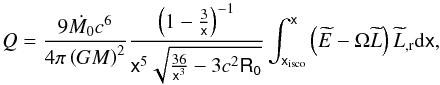 (74)where
 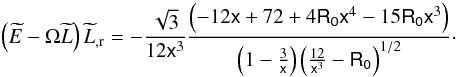 (75)We adopt for the radius of the outer edge of the disk (Dove et al. 1997):
  (76)According to the latter equation, if we take for the innermost stable circular orbit risco = 6.3rg, the outer egde of the disk yields approximately 70rg. If larger values of rout are considered, there are no major differences in the temperature and luminosity distributions.
We first compute the temperature and luminosity spectra distributions for R0 < 0, and adopt the values given in Table 2. In Figs. 14 and 15 we show the plots of the temperature as a function of the radial coordinate, and of the luminosity as a function of the energy, respectively. Notice that the corrections due to the gravitational redshift have been taken into account.
The maximum temperature as well as the luminosity increase for smaller values of R0 (Figs. 14 and 15). In the four cases presented, the accretion disk is hotter than in GR, e.g. in a f(R)-Schwarzschild disk for R0 = −1.5, the maximum temperature and luminosity are a factor 1.9 and 3.7, respectively, higher. The energy corresponding to the peak of the emission shifts to higher values, reaching 1359.20 eV for the set of adopted parameters.
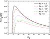 |
Fig. 14 Temperature as a function of the radial coordinate for some values of R0 < 0, for a f(R)-Schwarzschild black hole. |
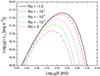 |
Fig. 15 Luminosity as a function of the energy for some values of R0 < 0, for a f(R)-Schwarzschild black hole. |
Values of the location of the last stable circular orbit, location in the radial coordinate of the maximum temperature, maximum temperature and luminosity, and the energy of the peak of the emission for an accretion disk around a f(R)-Schwarzschild black hole with R0 < 0.
We showed in Sect. 3.1.2 that for R0 > 0, stable circular orbits are possible within a minimum and maximum radius. We see in Table 1 that only for R0 = 10-12 and R0 = 10-6 accretion disks are possible, if we take for the radius of the outer edge of the disk rout = 70rg. The values of the location of the innermost stable circular orbit, location in the radial coordinate of the maximum temperature, maximum temperature and luminosity, and the energy of the peak of the emission are displayed in Table 7. We conclude that for R0 ∈ (0,10-6] the temperature and energy distributions have no significant differences with Schwarzschild’s distributions in GR.
Values of the location of the innermost stable circular orbit, location in the radial coordinate of the maximum temperature, maximum temperature and luminosity, and the energy of the peak of the emission for an accretion disk around a f(R)-Schwarzschild black hole with R0 > 0.
4.2.2. f(R)-Kerr black holes
We calculate next the energy flux of an accretion disk around a f(R)-Kerr black hole:  (77)where:
 ![Mathematical equation: \begin{eqnarray} &&\Omega_{,{\mathsf x}} = -36 \sqrt{3} \frac{c}{\mu^2}\eta , \\ &&\eta \equiv \frac{\mathsf{x}^{1/2}\left\{12\mathsf{x}^3+\mathsf{a}\left[12\mathsf{a}-\mathsf{a}\mathsf{R_0} \mathsf{x}^3-4\sqrt{36\mathsf{x}^3-3\mathsf{x}^6\mathsf{R_0}}\right]\right\}}{\left(12 \mathsf{x}^3+\mathsf{a}^2\mathsf{R_0}\mathsf{x}^3-12\mathsf{a}^2\right)^2\sqrt{-\mathsf{R_0} \mathsf{x}^3+12}}, \notag\\ &&\widetilde{L}=\frac{2 \mu\left(l_{1}+l_{2}\right)}{\left(12+\mathsf{a}^2 \mathsf{R_0}\right)\mathsf{x} \sqrt{{l_{3}+l_{4}}}}, \\ &&\widetilde{L}_{,{\mathsf x}}=-\frac{4 \mathsf{x}\left[12\mathsf{x}^3+\mathsf{a}^2\left(-12+\mathsf{R_0}\mathsf{x}^3\right)\right] \left( l_{5}+l_{6}+l_{7}+l_{8}+l_{9}\right)}{\left(12+\mathsf{a}^2 \mathsf{R_0}\right) \sqrt{12 \mathsf{x}^3-\mathsf{R_0} \mathsf{x}^6} \left(l_{10}+l_{11}\right)^{3/2}},~~~~~~ \\ &&\left(\widetilde{E}-\Omega\widetilde{L}\right) = \frac{12 c \sqrt{l_{3}+l_{4}}}{\left(12+\mathsf{a}^2 \mathsf{R_0}\right) \left[12 \mathsf{x}^3+\mathsf{a}^2 \left(-12 + \mathsf{x}^3 \mathsf{R_0}\right)\right]}, \end{eqnarray}](/articles/aa/full_html/2013/03/aa20378-12/aa20378-12-eq312.png) and
and ![Mathematical equation: \begin{eqnarray*} &&l_{1} = -72 \mathsf{a}^3 \mathsf{x}-216 \mathsf{a} \mathsf{x}^3+12 \mathsf{x}^3 \sqrt{36 \mathsf{x}^3-3 \mathsf{x}^6 \mathsf{R_0}},\\ &&l_{2} = \mathsf{a}^{2} \sqrt{36 \mathsf{x}^3-3 \mathsf{x}^6 \mathsf{R_0}}\:\left[\mathsf{a}^{2}\mathsf{x} \mathsf{R_0}+24+\mathsf{x}\left(12+\mathsf{x}^{2}\mathsf{R_0}\right)\right],\\ &&l_{3} = -432 \mathsf{a}^{2} \mathsf{x}^2+ \mathsf{x}^6 \left(12+\mathsf{a}^{2} \mathsf{R_0}\right)^2+48 \mathsf{a}^{3} \sqrt{36 \mathsf{x}^3-3 \mathsf{x}^6 \mathsf{R_0}},\\ &&l_{4} = 144 \mathsf{a} \mathsf{x}^2 \sqrt{36 \mathsf{x}^3-3 \mathsf{x}^6 \mathsf{R_0}}\\ &&\qquad -12 \mathsf{x}^3 \left[36 \mathsf{x}^2+\mathsf{a}^4 \mathsf{R_0}+\mathsf{a}^2 \left(36-3 \mathsf{x}^2 \mathsf{R_0}\right)\right],\\ &&l_{5} = \left[108\mathsf{a}\mathsf{x}^2\left(-24-12\mathsf{x}+5\mathsf{R_0}\mathsf{x}^3\right) \right]\sqrt{12\mathsf{x}^3-\mathsf{R_0}\mathsf{x}^6},\\ &&l_{6} = 36\mathsf{a}^3\left(-48-36\mathsf{x}+7\mathsf{R_0}\mathsf{x}^3\right)\sqrt{12\mathsf{x}^3- \mathsf{R_0}\mathsf{x}^6},\\ &&l_{7} = \sqrt{3}\mathsf{a}^4\mathsf{x}\left(-12+\mathsf{R_0}\mathsf{x}^3\right) \left[-108+\mathsf{R_0}\mathsf{x}^2\left(-3+\mathsf{R_0}\mathsf{x}^3\right)\right], \\ &&l_{8} = 36 \sqrt{3} \mathsf{x}^5 \left\{72+\mathsf{x}\left[-12+\mathsf{R_0}\mathsf{x}^2\left(-15+4\mathsf{x} \right)\right]\right\},\\ &&l_{9} = 3 \sqrt{3} \mathsf{a}^2 \mathsf{x}^2 \left\{864+\mathsf{x} l_{9a}\right\},\\ &&l_{9a}= \left[2160+\mathsf{x} l_{9a1}\right],\\ &&l_{9a1} = \left(432+\mathsf{R_0}^2\mathsf{x}^4\left(15+8\mathsf{x} \right)-12\mathsf{R_0}\mathsf{x}\left(21+26\mathsf{x}\right)\right),\\ &&l_{10} = 144\left(-3+\mathsf{x}\right)\mathsf{x}^5+\mathsf{a}^4\mathsf{R_0}\mathsf{x}^3 \left(-12+\mathsf{R_0}\mathsf{x}^3\right)\\ &&\qquad +48\mathsf{a}^3\sqrt{36\mathsf{x}^3-3\mathsf{R_0}\mathsf{x}^6},\\ &&l_{11} = 144\mathsf{a}\mathsf{x}^2\sqrt{36\mathsf{x}^3-3\mathsf{R_0}\mathsf{x}^6}+ 12\mathsf{a}^2\mathsf{x}^2l_{11a},\\ &&l_{11a} = -36+\mathsf{x}\left[-36+\mathsf{R_0}\mathsf{x}^2\left(3+2\mathsf{x}\right)\right]. \end{eqnarray*}](/articles/aa/full_html/2013/03/aa20378-12/aa20378-12-eq313.png) If we adopt for the radius of the inner edge of the disk 1.4545rg, according to Eq. (76), rout ≈ 16rg. From Eq. (77) we numerically calculate the temperature and luminosity for the values shown in Table 3, taking into account the corrections coming from the gravitational redshift. The results are displayed in Figs. 16, 17, and Table 8. We see that the temperature of the disk increases for smaller values of R0. The ratio of the maximum temperature between the GR and f(R) cases, with R0 = −1.25 × 10⁻¹, is 1.20. The peak of the emission rises a factor of 2, and the corresponding energy is shifted towards higher energies.
If we adopt for the radius of the inner edge of the disk 1.4545rg, according to Eq. (76), rout ≈ 16rg. From Eq. (77) we numerically calculate the temperature and luminosity for the values shown in Table 3, taking into account the corrections coming from the gravitational redshift. The results are displayed in Figs. 16, 17, and Table 8. We see that the temperature of the disk increases for smaller values of R0. The ratio of the maximum temperature between the GR and f(R) cases, with R0 = −1.25 × 10⁻¹, is 1.20. The peak of the emission rises a factor of 2, and the corresponding energy is shifted towards higher energies.
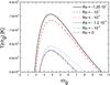 |
Fig. 16 Temperature as a function of the radial coordinate for some values of R0 < 0 of a f(R)-Kerr black hole of angular momentum a = 0.99, corrected by gravitational redshift. |
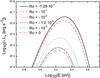 |
Fig. 17 Luminosity as a function of the energy for some values of R0 < 0, for a f(R)-Kerr black hole of angular momentum a = 0.99. |
Location of the last stable circular orbit and maximum temperature, maximum temperature, luminosity, and energy of the peak of the emission for an accretion disk around a f(R)-Kerr black hole with R0 < 0 and a = 0.99.
Values of the location of the last stable circular orbit, location in the radial coordinate of the maximum temperature, maximum temperature and luminosity, and the energy of the peak of the emission for an accretion disk around a f(R)-Kerr black hole with R0 > 0 and a = 0.99.
Since the radius of the outer edge of the disk is 16rg, we see from Table 4 that accretion disks are only possible for R0 = 10-6 and R0 = 10-4, until up R0 = 6.67 × 10⁻⁴. For such values of R0, we show in Table 9 the values of the location of the last stable circular orbit, maximum temperature, luminosity, and the energy of the peak of the emission, and in Figs. 18 and 19, the temperature and luminosity distributions respectively. As in f(R)-Schwarzschild black holes with positive Ricci scalar, these differences are minor.
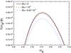 |
Fig. 18 Temperature as a function of the radial coordinate for some values of R0 > 0, for a f(R)-Kerr black hole of angular momentum a = 0.99. |
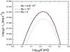 |
Fig. 19 Luminosity as a function of the energy for some values of R0 > 0, for a f(R)-Kerr black hole of angular momentum a = 0.99. |
We proceed now to examine some specific forms of the function f, and the constraints imposed on them by the previous analysis.
5. Limits on specific prescriptions for f(R)
As discussed in Sects. 3.1.2 and 3.2.2, the existence of Page-Thorne disks around f(R) black holes imposes the following limits on R0:
-
f(R)-Schwarzschild space-time:
![Mathematical equation: \begin{equation} \label{cond3} \mathsf{R}_{0} \in (-\infty ;10^{-6}], \end{equation}](/articles/aa/full_html/2013/03/aa20378-12/aa20378-12-eq356.png) (82)
(82) -
f(R)-Kerr space-time:
![Mathematical equation: \begin{equation} \label{cond4} \mathsf{R}_{0} \in \left[-1.2\times10^{-3} ; 6.67\times10^{-4}\right]. \end{equation}](/articles/aa/full_html/2013/03/aa20378-12/aa20378-12-eq357.png) (83)
(83)
 (84)
(84) (85)
(85)
5.1. f(R) = α Rβ
The parameters α, β and the Ricci scalar are related by Eq. (7) as follows: ![Mathematical equation: \begin{equation} R_0 = \left[\frac{1}{\alpha \left(\beta-2\right)}\right]^{\frac{1}{\beta-1}}\cdot \end{equation}](/articles/aa/full_html/2013/03/aa20378-12/aa20378-12-eq363.png) (86)Introducing the adimensional parameter
(86)Introducing the adimensional parameter  with
with  , this equation can be written as
 ![Mathematical equation: \begin{equation} \mathsf{R}_0 = \left[\frac{1}{\alpha ' \left(\beta-2\right)}\right]^{\frac{1}{\beta-1}}\cdot \label{86} \end{equation}](/articles/aa/full_html/2013/03/aa20378-12/aa20378-12-eq366.png) (87)Notice the condition β > 0 to ensure the GR limit for small values of the Ricci scalar R. Let us consider first the case of a positive Ricci scalar, which leads to:
(87)Notice the condition β > 0 to ensure the GR limit for small values of the Ricci scalar R. Let us consider first the case of a positive Ricci scalar, which leads to:
Case I  (88)or
  (89)
(89)
Case II  (90)or
  (91)and 1/(β − 1) an even number, that is:
  (92)with n ∈ Z. By isolating α′ from Eq. (87), we obtain the function:
 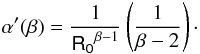 (93)We show in Fig. 20 the plot of α′ as a function of β (with β > 0) for fixed values of the Ricci scalar. We see that for β ∈ (0,2), α′ ∈ (−∞,0). For β = 2, Eq. (93) is not defined, while for β > 2, α′ takes large positive values. Since α needs to be small in order to recover GR for small values of the Ricci scalar, the case α′ > 0, β > 2 is discarded. Hence, we obtain the following restrictions on the parameters:
![Mathematical equation: \hbox{$\alpha '\in (-\infty ;0)\:\:\:\wedge\:\:\:\beta \in (0 ;2)\:\:\:\wedge\:\:\:\mathsf{R}_0 \in (0 ;6.67\times 10^{-4}].$}](/articles/aa/full_html/2013/03/aa20378-12/aa20378-12-eq113.png)
For negative values of the Ricci scalar, from Eq. (93) we require that:  (94)or:
  (95)where
  , so that β > 0. If m = 0, β = 1 and α′ = α = −1. These values of the parameters lead to f(R) = −R, which does not reduce to GR. For β = 2, Eq. (93) is not defined. If β ≥ 3 and is an odd number, α′ takes positive large values, while if β ≥ 4 and is an even number α′ is large and negative. Since α′ has to be small to recover GR for small values of the Ricci scalar, we conclude that negative values of R0 are not allowed in this theory.
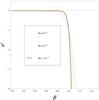 |
Fig. 20 α′ as a function of β for different values of R0. |
We now restrict the values of α and β according to Eqs. (84) and (85). The first and second derivative for the given f function are: 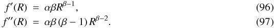 The restrictions over α and β that satisfy Eq. (85) are:
  (98)or
  (99)The condition given by Eq. (98) is discarded because it does not satisfy Eq. (93). The viability condition expressed by Eq. (84) takes the form:
  (100)We can constrain the values of α using the latter inequality as follows:
  By multiplying by R0β − 1α the latter restrictions yields:
  (101)In order to satisfy Eq. (100):
  If β = 0, α > − R0, and for β = 1, α > − 1. The set of values for α is α ∈ ( − R0,0).
We conclude that the values of α and β that are permitted by our model as well as by the two viability conditions are:
![Mathematical equation: \hbox{$\\alpha \in (-R_0 ;0)\:\:\:\wedge\:\:\:\beta \in (0 ;1)\:\:\:\wedge\:\:\:\mathsf{R_0} \in (0 ;6.67\times 10^{-4}].$}](/articles/aa/full_html/2013/03/aa20378-12/aa20378-12-eq114.png)
5.2. f(R) = R ϵ
In this case, the parameters ϵ and α, and the Ricci scalar are related by Eq. (7) in the simple form:  (102)Dividing by Rg, we obtain
  . For R0 > 0, the function α′(ϵ) is always positive, while it is negative for all ϵ if R0 < 0. The constrains over ϵ and α that follow from Eq. (7) are:
-
R0 ∈ (0;6.67 × 10⁻⁴]
 or
or 
-
R0 ∈ [−1.2 × 10⁻³;0)
 or
or 
 The condition f′′(R0) > 0 is satisfied if ϵ > 0 ∧ R0 > 0, or ϵ < 0 ∧ R0 < 0. Equation (84) in adimensional form is:
  (105)This equation, together with (104), yields:
-
For ϵ > 0 and R0 > 0,
 .
. -
For ϵ < 0 and R0 < 0,
![Mathematical equation: \begin{eqnarray} \mathsf{R_0} & \in &(0 ;6.67\times 10^{-4}],\;\;\;\;\epsilon >0,\;\;\;\;\alpha '\in (e^{-1}\;\mathsf{R_0} ; \infty),\\ \nonumber \alpha ' & \in & \left(e\;\mathsf{R_0} ; \mathsf{R_0}\exp\left\{\left(\frac 1 \epsilon +1\right)\right\}\right), \nonumber \end{eqnarray}](/articles/aa/full_html/2013/03/aa20378-12/aa20378-12-eq427.png) (106)and
(106)and  (107)The first group of constraints is fulfilled for ϵ > 0, while in the second group for only ϵ ∈ (−1/2,0). We conclude that for the f(R) under scrutiny, the values
 ![Mathematical equation: \begin{equation} \mathsf{R_0} \in (0 ;6.67\times 10^{-4}],\;\;\;\;\epsilon >0,\;\;\;\;\alpha '\in (e \;\mathsf{R_0} ; \infty), \end{equation}](/articles/aa/full_html/2013/03/aa20378-12/aa20378-12-eq431.png) (108)and,
(108)and,  (109)are allowed.
6. Discussion
The results presented in Sect. 4 can be compared with current observational data to derive some constraints on a given f(R) theory. In order to illustrate this assertion we shall consider Cygnus X-1, which is the most intensively studied black hole binary system in the Galaxy. A series of recent high-quality papers (Reid et al. 2011; Orosz et al. 2011; Gou et al. 2011) have provided an unprecedented set of accurate measurements of the distance, the black hole mass, spin parameter a, and the orbital inclination of this source. This opens the possibility to constrain modified theories of gravity with rather local precision observations of astrophysical objects in the Galaxy.
Cygnus X-1 was discovered at X-rays by Bowyer et al. (1965). Early dynamical studies of the compact object suggested the presence of an accreting black hole (e.g. Bolton 1972). The distance to Cygnus X-1 is currently estimated to be  kpc (Reid et al. 2011). This value was determined via trigonometric parallax using the Very Long Baseline Array (VLBA). At this distance, the mass of the black hole is (Orosz et al. 2011) M = 14.8 M⊙. This is the value adopted in all calculations presented in the previous sections.
The source has been observed in both a low-hard state, dominated by the emission of a hot corona (e.g., Dove et al. 1997; Gierlinski et al. 1997; Poutanen 1998), and a high-soft state, dominated by the accretion disk, which in this state goes all the way down to the last stable orbit. In the low-hard state, where the source spends most of the time, a steady, non-thermal jet is observed (Stirling et al. 2001). The jet is absent in the thermal state. Therefore, in this latter state a clearer X-ray spectrum can be obtained.
The accretion rate and the spin parameter of the hole are ~ 0.472 × 10¹⁹ g s-1 and 0.99, respectively, according to estimates from a Kerr plus black-body disk model (Gou et al. 2011). These GR models yield a spectral energy distribution with a maximum at Emax ~ 1.6 keV. On the contrary, f(R)-models with negative curvature correspond to a low maximum temperature, lower even than what is expected for the (unrealistic) case of a Schwarzschild black hole. Therefore, we can presume that a fit of f(R)-Kerr models to the data would also prefer high values of maximum temperature, i.e., ones with non-negative curvature. Models with accretion rates and spin close to those obtained by Gou et al. (2011) and small positive curvature seem viable, something that is consistent with an asymptotic behaviour corresponding to a de Sitter space-time endowed with a small and positive value of the cosmological constant.
Deep X-ray studies with Chandra satellite might impose more restrictive limits, especially if independent constraints onto the accretion rate become available.
7. Conclusions
We have studied stable circular orbits and relativistic accretion disks around Schwarzschild and Kerr black holes in f(R) gravity with constant Ricci curvature in the strong regime. We have found that stable disks can be formed only for curvatures in the ranges of ( − ∞,10-6] and [ − 1.2 × 10-3,6.67 × 10-4] in the cases of Schwarzschild and Kerr black holes, respectively. Current observations of Cygnus X-1 in the soft state rule out curvature values below − 1.2 × 10⁻³. Additional constrains can be imposed on specific prescriptions of f(R) gravity. In particular, logaritmic-gravity prescriptions are strongly constrained by observational data. Future high-precision determination of the parameters of other black hole candidates can be used to impose more restrictive limits to extended theories of gravity.
Accretion through thick disks onto Schwarzschild and Kerr black holes with a repulsive cosmological constant was studied by Rezzolla et al. (2003), and Slaný & Stuchlík (2005), respectively. These studies do not analyze spectra or compare results with observational data.
The results obtained in our analysis of f(R)-Schwarzschild space-time with constant Ricci scalar are consistent with those given by Stuchlík & Hledík (1999) in Schwarzschild-de Sitter and Schwarzschild-anti de Sitter space-times.
Here H represents a particular height above the central plane of the disk (|z| ≤ H ≪ r).
Acknowledgments
We are grateful to an anonymous referee for useful suggestions. BH astrophysics with G.E. Romero is supported by grant PIP 2010/0078 (CONICET). Additional funds comes from Ministerio de Educación y Ciencia (Spain) trhough grant AYA 2010-21782-C03-01. S.E.P.B. acknowledges support from UERJ, FAPERJ, and ICRANet-Pescara. We thank Gabriela Vila and Florencia Vieyro for comments on accretion disks.
References
- Abdelwahab, M., Goswami, R., & Dunsby, P. 2012, Phys. Rev. D, 85, 083511 [NASA ADS] [CrossRef] [Google Scholar]
- Arbuzova, E. V., Dolgov, A. D., & Reverberi, L. 2012, JCAP, 02, 04 [Google Scholar]
- Biswas, T., Cembranos, J. A. R., & Kapusta, J. I. 2010, Phys. Rev. Lett., 104, 021601 [NASA ADS] [CrossRef] [Google Scholar]
- Biswas, T., Cembranos, J. A. R., & Kapusta, J. I. 2010, JHEP, 1010, 048 [NASA ADS] [Google Scholar]
- Bolton, C. T. 1972, Nat. Phys. Sci., 240, 124 [NASA ADS] [CrossRef] [Google Scholar]
- Bowyer, S., Byram, E. T., Chubb, T. A., & Friedman, H. 1965, Science, 147, 394 [NASA ADS] [CrossRef] [Google Scholar]
- Capozziello, S. 2002, Int. J. Mod. Phys. D, 11, 483 [Google Scholar]
- Capozziello S., & Faraoni V. 2010, Beyond Einstein Gravity. A survey of Gravitational Theories for Cosmology and Astrophysics (Dordrecht-Heidelberg-London-New York: Springer) [Google Scholar]
- Carter, B. 1973, in Les Astres Occlus eds. C. DeWitt, & B. DeWitt (New York, Gordon & Breach) [Google Scholar]
- Cembranos, J. A. R., de la Cruz-Dombriz, A., & Jimeno Romero, P. 2011 [arXiv:1109.4519v1] [Google Scholar]
- Cooney, A., DeDeo, S., & Psaltis, D. 2010, Phys. Rev. D, 82, 064033 [NASA ADS] [CrossRef] [Google Scholar]
- De Felice, A., & Tsujikawa, S. 2010, Living Rev. Relat., 13 3 [Google Scholar]
- de la Cruz-Dombriz, A., Dobado, A., & Maroto, A. L. 2009, Phys. Rev. D, 80, 124011; Erratum-ibid, 2011, 83, 029903 [NASA ADS] [CrossRef] [Google Scholar]
- Dove, J. B., Wilms, J., Maisack, M., & Begelman, M. 1997, ApJ, 487, 759 [NASA ADS] [CrossRef] [Google Scholar]
- Gierlinski, M., Zdziarski, A. A., Done, C., et al. 1997, MNRAS, 228, 958 [NASA ADS] [CrossRef] [Google Scholar]
- Gou, L., McClintock, J. E., Reid, Mark, J., et al. 2011, ApJ, 742, 85 [NASA ADS] [CrossRef] [Google Scholar]
- Harko, T., Kovács, Z., & Lobo, F. N. N. 2009, Phys. Rev. D, 79, 064001 [NASA ADS] [CrossRef] [MathSciNet] [Google Scholar]
- Hendi, S. H., & Momeni, D. 2011, Eur. Phys. J. C, 71, 1823 [Google Scholar]
- Hendi, S. H., Panah, B. E., & Mousavi, S. M. 2012, Gen. Rel. Grav., 44, 835 [Google Scholar]
- Hobson, M. P., Estathoiou, G. P., & Lasenby, A. N. 2006, General Relativity. An Introduction for Physicists (Cambridge: Cambridge, University Press) [Google Scholar]
- Kerr, R. P. 1963, Phys. Rev. Lett., 11, 237 [NASA ADS] [CrossRef] [MathSciNet] [Google Scholar]
- Li, M., Li, X., & Wang, S. 2011, Commun. Theor. Phys., 56, 525 [NASA ADS] [CrossRef] [Google Scholar]
- Magnano, G., Ferraris, M., & Francaviglia, M. 1987, Gen. Rel. Gravit., 19, 465 [Google Scholar]
- Mazharimousavi, H. S., Halilsay, M., & Tahamtan, T. 2012, Eur. Phys. J. C, 72, 1851 [NASA ADS] [CrossRef] [EDP Sciences] [Google Scholar]
- Moon, T., Myung, Y. S., & Son, E. J. 2011a, Gen. Rel. Gravit., 43, 3079 [Google Scholar]
- Moon, T., Myung, Y. S., & Son, E. J. 2011b, Eur. Phys. J., C71, 1777 [Google Scholar]
- Motohashi, H., & Nishizawa, A. 2012, Phys. Rev. D, 86, 083514 [NASA ADS] [CrossRef] [Google Scholar]
- Myung, Y. S. 2011, Phys. Rev. D, 84, 024048 [NASA ADS] [CrossRef] [Google Scholar]
- Myung, Y. S., Moon, T., & Son, E. J. 2011, Phys. Rev. D, 83, 124009 [NASA ADS] [CrossRef] [Google Scholar]
- Novikov, I. D., & Thorne, K. S. 1973, in Black Holes, eds. C. DeWitt, & B. DeWitt (New York: Gordon & Breach) [Google Scholar]
- Orosz, J. A., McClintock, J. E., Aufdenberg, J. P., et al. 2011, ApJ, 742, 84 [NASA ADS] [CrossRef] [Google Scholar]
- Page, D. N., & Thorne, K. S. 1974, ApJ, 191, 499 [NASA ADS] [CrossRef] [Google Scholar]
- Perez Bergliaffa, S. E., & Yves De Oliveira, E. 2011, Phys. Rev. D, 84, 084006 [NASA ADS] [CrossRef] [Google Scholar]
- Poutanen, J. 1998, Theory of Black Hole Accretion Disks, eds. M. A. Abramowicz, Gunnlaugur Bjornsson, and James E. Pringle. (Cambridge: Cambridge University Press) [Google Scholar]
- Psaltis, D., Perrodin, D., Dienes, K. R., & Mocioiu, I. 2008a, Phys. Rev. Lett., 100, 091101 [Google Scholar]
- Psaltis, D., Perrodin, D., Dienes, K. R., & Mocioiu, I. 2008b, Phys. Rev. Lett., 100, 119902 [NASA ADS] [CrossRef] [Google Scholar]
- Pun, C. S., Zovács, Z., & Harko, T. 2008, Phys. Rev. D, 78, 024043 [NASA ADS] [CrossRef] [Google Scholar]
- Reid, M. J., McClintock, J. E., Narayan, R., et al. 2011, ApJ, 742, 83 [NASA ADS] [CrossRef] [Google Scholar]
- Rezzolla, L., Zanotti, O., & Font, J. A. 2003, A&A, 412, 603 [NASA ADS] [CrossRef] [EDP Sciences] [Google Scholar]
- Schwarzschild, K. 1916, Sitzungsberichte der Königlich-Preussischen Akademie der Wissenschaften, 3, 189 [Google Scholar]
- Shakura, N. I., & Sunyaev, R. A. 1973, A&A, 24, 377 [Google Scholar]
- Sotiriou, T. P., & Faraoni, V. 2010, Rev. Mod. Phys., 82, 451 [NASA ADS] [CrossRef] [MathSciNet] [Google Scholar]
- Starobinsky, A. A. 1980, Phys. Lett. B, 91, 99 [NASA ADS] [CrossRef] [Google Scholar]
- Stirling, A. M., Spencer, R. E., de la Force, C. J., et al. 2001, MNRAS, 327, 1273 [NASA ADS] [CrossRef] [Google Scholar]
- Stuchlík, Z., & Hledík, S. 1999, Phys. Rev. D, 60, 044006 [NASA ADS] [CrossRef] [MathSciNet] [Google Scholar]
- Stuchlík, Z., & Slaný, P. 2004, Phys. Rev. D, 69, 064001 [NASA ADS] [CrossRef] [Google Scholar]
- Slaný, P., & Stuchlík, Z. 2005, Class. Quant. Grav., 22, 3623 [Google Scholar]
- Weinberg, S. 1989, Rev. Mod. Phys., 61, 1 [NASA ADS] [CrossRef] [MathSciNet] [Google Scholar]
- Will, C. M. 2006, Living Rev. Relat., 9, 3 [Google Scholar]
All Tables
Location of the event and cosmological horizon, and of the innermost and outermost stable circular orbits for R0 > 0 in f(R)-Schwarzschild space-time.
Location of the event horizon, and of the innermost stable circular orbit for R0 < 0 in f(R)-Schwarzschild space-time.
Radii of event horizons and circular orbits for a f(R)-Kerr black hole of angular momentum a = 0.99, for some values of R0 < 0.
Location of the event and cosmological horizon, and of the innermost and outermost stable circular orbits for R0 > 0 and a = 0.99 in f(R)-Kerr space-time.
Values of the energy of the peak of the emission, the maximum temperature, and luminosity of an accretion disk around Schwarzschild and Kerr black holes (a = 0.99) in the SS and PT models.
Values of the location of the last stable circular orbit, location in the radial coordinate of the maximum temperature, maximum temperature and luminosity, and the energy of the peak of the emission for an accretion disk around a f(R)-Schwarzschild black hole with R0 < 0.
Values of the location of the innermost stable circular orbit, location in the radial coordinate of the maximum temperature, maximum temperature and luminosity, and the energy of the peak of the emission for an accretion disk around a f(R)-Schwarzschild black hole with R0 > 0.
Location of the last stable circular orbit and maximum temperature, maximum temperature, luminosity, and energy of the peak of the emission for an accretion disk around a f(R)-Kerr black hole with R0 < 0 and a = 0.99.
Values of the location of the last stable circular orbit, location in the radial coordinate of the maximum temperature, maximum temperature and luminosity, and the energy of the peak of the emission for an accretion disk around a f(R)-Kerr black hole with R0 > 0 and a = 0.99.
All Figures
|
Fig. 1 Ricci scalar as a function of the radial coordinate of the event horizon in f(R)-Schwarzschild space-time. |
| In the text | |
|
Fig. 2 Function given by Eq. (23). The absolute maximum corresponds to x = 15/2 and R0 = 2.85 × 10⁻³. |
| In the text | |
|
Fig. 3 Effective potential for different values of R0 > 0 and h in f(R)-Schwarzschild space-time. The dots indicate the location of the innermost stable circular orbit. |
| In the text | |
|
Fig. 4 Ricci scalar as a function of the radial coordinate of the event horizon (line) and of the Ricci scalar as a function of the radial coordinate of the innermost stable circular orbits (dashed line) for R0 ∈ [ − 1.5,0.45] in f(R)-Schwarzschild space-time. |
| In the text | |
|
Fig. 5 Effective potential for different values of R0 < 0 and h in f(R)-Schwarzschild space-time. The dots indicate the location of the innermost stable circular orbit. |
| In the text | |
|
Fig. 6 Ricci scalar as a function of the radial coordinate of the event horizon for R0 ∈ [ − 0.3,1] and a = 0.99 in f(R)-Kerr space-time. |
| In the text | |
|
Fig. 7 Effective potential as a function of the radial coordinate (R0 < 0, a = 0.99), in f(R)-Kerr space-time. The dots indicate the location of the innermost stable circular orbit. |
| In the text | |
|
Fig. 8 Effective potential as a function of the radial coordinate (R0 > 0, a = 0.99), in f(R)-Kerr space-time. The dots indicate the location of the innermost stable circular orbit. |
| In the text | |
|
Fig. 9 Energy flux as a function of the radial coordinate of an accretion disk around a Schwarzschild black hole in Shakura-Sunyaev (SS) and Page-Thorne (PT) models, respectely. |
| In the text | |
|
Fig. 10 Temperature as a function of the radial coordinate of an accretion disk around a Schwarzschild black hole in SS and PT models, respectively. |
| In the text | |
|
Fig. 11 Energy flux as function of the radial coordinate for an accretion disk around a Kerr black hole of angular momentum a = 0.99 in the PT model. |
| In the text | |
|
Fig. 12 Temperature as function of the radial coordinate of an accretion disk around a Kerr black hole of angular momentum a = 0.99 in the PT model. |
| In the text | |
|
Fig. 13 Luminosity as function of the energy for a relativistic accretion disk around a Schwarzschild and a Kerr black hole (a = 0.99). We also plot the luminosity as a function of the energy of an accretion disk around a Schwarzschild black hole that corresponds to the SS model. |
| In the text | |
|
Fig. 14 Temperature as a function of the radial coordinate for some values of R0 < 0, for a f(R)-Schwarzschild black hole. |
| In the text | |
|
Fig. 15 Luminosity as a function of the energy for some values of R0 < 0, for a f(R)-Schwarzschild black hole. |
| In the text | |
|
Fig. 16 Temperature as a function of the radial coordinate for some values of R0 < 0 of a f(R)-Kerr black hole of angular momentum a = 0.99, corrected by gravitational redshift. |
| In the text | |
|
Fig. 17 Luminosity as a function of the energy for some values of R0 < 0, for a f(R)-Kerr black hole of angular momentum a = 0.99. |
| In the text | |
|
Fig. 18 Temperature as a function of the radial coordinate for some values of R0 > 0, for a f(R)-Kerr black hole of angular momentum a = 0.99. |
| In the text | |
|
Fig. 19 Luminosity as a function of the energy for some values of R0 > 0, for a f(R)-Kerr black hole of angular momentum a = 0.99. |
| In the text | |
|
Fig. 20 α′ as a function of β for different values of R0. |
| In the text | |
Current usage metrics show cumulative count of Article Views (full-text article views including HTML views, PDF and ePub downloads, according to the available data) and Abstracts Views on Vision4Press platform.
Data correspond to usage on the plateform after 2015. The current usage metrics is available 48-96 hours after online publication and is updated daily on week days.
Initial download of the metrics may take a while.