| Issue |
A&A
Volume 551, March 2013
|
|
|---|---|---|
| Article Number | A124 | |
| Number of page(s) | 11 | |
| Section | Stellar structure and evolution | |
| DOI | https://doi.org/10.1051/0004-6361/201220023 | |
| Published online | 05 March 2013 | |
Prompt thermal emission in gamma-ray bursts
1
UPMC-CNRS, UMR 7095, Institut d’Astrophysique de Paris,
75014
Paris,
France
e-mail: hascoetiap.fr; daigneiap.fr; This email address is being protected from spambots. You need JavaScript enabled to view it.
2
Physics Department and Astronomy Department, Columbia
University, 538 West 120th
Street, New York,
NY
10027,
USA
3 Institut Universitaire de France
Received:
16
July
2012
Accepted:
22
January
2013
Abstract
Context. Gamma-ray burst (GRB) spectra globally appear non-thermal, but recent observations of a few bursts with Fermi GBM have confirmed previous indications from BATSE of the presence of an underlying thermal component. Photospheric emission is indeed expected when the relativistic outflow emerging from the central engine becomes transparent to its own radiation, with a quasi-blackbody spectrum in absence of additional sub-photospheric dissipation. However, its intensity strongly depends on the acceleration mechanism – thermal or magnetic – of the flow.
Aims. We aim to compute the thermal and non-thermal emissions (light curves and spectra) produced by an outflow with a variable Lorentz factor, where the power Ėiso injected at the origin is partially thermal (fraction ϵth ≤ 1) and partially magnetic (fraction 1−ϵth). The thermal emission is produced at the photosphere, and the non-thermal emission in the optically thin regime. Apart from the value of ϵth, we want to test how the other model parameters affect the observed ratio of the thermal to non-thermal emission.
Methods. We followed the adiabatic cooling of the flow from the origin to the photosphere and computed the emitted radiation, which is a sum of modified black bodies at different temperatures (as the temperature strongly depends on the Lorentz factor of each shell at transparency). If the non-thermal emission comes from internal shocks, it is obtained from a multi-shell model where a fraction of the energy dissipated in shell collision is transferred to electrons and radiated via the synchrotron mechanism. If, conversely, the non-thermal emission originates in magnetic reconnection, the lack of any detailed theory for this process forced us to use a very simple parametrisation to estimate the emitted spectrum.
Results. If the non-thermal emission is made by internal shocks, we self-consistently obtained the light curves and spectra of the thermal and non-thermal components for any distribution of the Lorentz factor in the flow. If the non-thermal emission results from magnetic reconnection we were unable to produce a light curve and could only compare the respective non-thermal and thermal spectra. In the different considered cases, we varied the model parameters to see when the thermal component in the light curve and/or spectrum is likely to show up or, on the contrary, to be hidden. We finally compared our results to the proposed evidence for the presence of a thermal component in GRB spectra. Focussing on GRB 090902B and GRB 10072B, we showed how these observations can be used to constrain the nature and acceleration mechanism of GRB outflows.
Key words: gamma-ray burst: general / radiation mechanisms: thermal / radiation mechanisms: non-thermal / shock waves / magnetic reconnection
© ESO, 2013
1. Introduction
The first gamma-ray burst (GRB) spectra were obtained by the gamma and X-ray spectrometers on board the IMP-6 satellite and the Apollo 16 spacecraft (Cline et al. 1973; Metzger et al. 1974). These early observations were complemented by the large sample of 143 spectra collected by the Konus experiments on the Venera probes from 1978 to 1980 (Mazets et al. 1981). It was shown that these spectra could be fitted by a power law with an exponential cutoff or a broken power law (Cline & Desai 1975), and various physical processes were invoked to explain this shape, such as optically-thin thermal bremsstrahlung (Gilman et al. 1980), Compton scattering of soft photons by non-thermal electrons (Zdziarski & Lamb 1986) or synchrotron emission by thermal or non-thermal electrons (Brainerd & Lamb 1987). Following the launch of the Compton Gamma-Ray Observatory, the Burst and Transient Source Experiment (BATSE) provided the first solid indications that GRBs were located at cosmological distances and confirmed the broken power law shape of the spectra that was represented by the phenomenological Band function (Band et al. 1993). Possible cyclotron or annihilation lines found by previous experiments were not seen by BATSE.
In the context of the cosmological models that were developed hereafter, the spectra were generally interpreted in terms of synchrotron emission from shock accelerated electrons (see e.g. Piran 1999) and therefore believed to be mostly non-thermal. The possibility that a thermal contribution could also be present was, however, considered by Mészáros et al. (2002), and was supported by several observational indications. The first one came from the very hard low-energy spectral slopes that are found in some BATSE bursts during at least part of the evolution (Preece et al. 1998; Ghirlanda et al. 2003). While the commonly observed value of the low-energy spectral index is α ~ −1, it reaches 0.5 to 1 in these events, suggesting the presence of a Rayleigh-Jeans contribution. Then Ryde (2004, 2005) proposed to fit all GRB spectra in the BATSE range with the combination of a thermal and a power law component. Using a time resolved analysis, he showed that during a pulse the temperature first stays approximately constant before decaying as a power law of temporal index close to −2/3.
In the previous examples the identified thermal component represented a major contribution responsible for the peak of the E2N(E) spectrum. A different result was obtained by Guiriec et al. (2011) who found a sub-dominant thermal component in the Fermi-Gamma-ray Burst Monitor (GBM) spectrum of GRB 100724B, accounting for a few percents of the energy released by the burst. The evolution of the temperature was not correlated to the peak energy of the non-thermal component, fitted by a Band function. Similar results have been found in other bright GBM bursts, such as GRB 110721A (Ryde et al. 2012), GRB 081207, and GRB 110920 (McGlynn et al. 2012). This improved characterisation of thermal components in the prompt emission of GRBs is allowed by the larger spectral coverage of GBM (8 keV–40 MeV) compared to BATSE (20 keV–2 MeV), leading to a better quality of the spectral fits.
On the theoretical side, a thermal emission originating from the photosphere is a natural prediction of most models based on the generic fireball scenario (Paczynski 1986; Goodman 1986; Shemi & Piran 1990; Mészáros et al. 1993). Moreover, if the acceleration of the outflow has a thermal origin (as would be the case if it was powered at its basis by neutrino-antineutrino annihilation), this photospheric emission would be very bright, outshining the non-thermal emission produced by internal shocks in the 100 keV–1 MeV spectral range (Daigne & Mochkovitch 2002). One is therefore faced with the following alternative: either most of the emission we observe is indeed this thermal component, but it has been Comptonised to produce a power law tail in the spectrum at high energy (see e.g. Thompson 1994; Rees & Mészáros 2005; Giannios & Spruit 2007; Beloborodov 2010) and complemented at low energy by additional processes (e.g. Pe’er et al. 2006; Vurm et al. 2011), or the acceleration has a magnetic origin (see e.g. Begelman & Li 1994; Daigne & Drenkhahn 2002; Vlahakis & Königl 2003; Komissarov et al. 2009; Tchekhovskoy et al. 2010; Komissarov et al. 2010; Granot et al. 2011) and the fraction ϵth of thermal energy in the flow is much smaller than unity.
In this work we explore the consequences of this second possibility. We self-consistently compute the photospheric thermal emission and the non-thermal emission from internal shocks. If the internal dissipation is dominated by magnetic reconnection rather than internal shocks, we get the non-thermal spectrum in a very simple parametrised way. We discuss the conditions for the thermal emission to show up or, on the contrary, to be hidden. The paper is organised as follows: in Sect. 2 we describe the geometry and thermodynamics of the flow and explain our method to compute the photospheric and non-thermal emissions; our results are presented in Sect. 3 and discussed in Sect. 4. Finally, Sect. 5 is the conclusion.
2. Model description
2.1. Geometry and thermodynamics of the flow
We consider a schematic model where the flow that emerges from the central engine is
accelerated by the conversion of thermal and/or magnetic energy to kinetic energy. We do
not specify the initial geometry of the flow (which can be largely governed by magnetic
forces), but we assume that beyond a radius Rsph it becomes
spherically symmetric within a cone of half opening angle θ. We also
define the radius Rsat, where the acceleration is essentially
complete and suppose that
Rsph < Rsat.
The total injected power in the flow is Ė, with a fraction
ϵth in thermal form. The temperature
T0 at the origin of the flow can then be obtained from
 (1)where
Ėiso and
S0 = πℓ2 are,
respectively, the isotropic injected power and the section of the flow at the origin (see
Fig. 1). The fraction of solid angle is
(1)where
Ėiso and
S0 = πℓ2 are,
respectively, the isotropic injected power and the section of the flow at the origin (see
Fig. 1). The fraction of solid angle is
 (we
count only one jet to be consistent with the definition of S0)
and a is the radiation constant. We finally get
(we
count only one jet to be consistent with the definition of S0)
and a is the radiation constant. We finally get  (2)with the opening
angle, injected power, and radius of the jet in units of 0.1 rad, 1053
erg s-1, and 107 cm, respectively.
(2)with the opening
angle, injected power, and radius of the jet in units of 0.1 rad, 1053
erg s-1, and 107 cm, respectively.
We obtain the flow equations assuming that no dissipation takes place below the
photosphere (so that the emerging spectrum at transparency will be thermal only). Mass and
entropy conservation then lead to 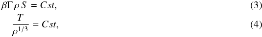 where
ρ is the comoving density, S the surface perpendicular
to the flow,
β = v/c, and
Γ = (1 − β2)−1/2. From Eqs.
(3), (4) we get
where
ρ is the comoving density, S the surface perpendicular
to the flow,
β = v/c, and
Γ = (1 − β2)−1/2. From Eqs.
(3), (4) we get  (5)Using Eq. (5) we can obtain the temperature at any radius
R > Rsph even if we
ignore the details of the geometry from the basis of the flow up to
Rsph. With
S(R) = π θ2 R2
and assuming that β ~ 1 already close to the origin we have
(5)Using Eq. (5) we can obtain the temperature at any radius
R > Rsph even if we
ignore the details of the geometry from the basis of the flow up to
Rsph. With
S(R) = π θ2 R2
and assuming that β ~ 1 already close to the origin we have
 (6)so that, in
the observer frame
(6)so that, in
the observer frame  (7)where
z is the burst redshift.
(7)where
z is the burst redshift.
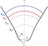 |
Fig. 1 Schematic view of the problem geometry. The flow emerges from the central engine through a “circular opening” of radius ℓ. Beyond a radius Rsph it expands radially within a cone of half opening θ. The acceleration is completed at Rsat. The photosphere is located at Rph and dissipation of kinetic and/or magnetic energy takes place at Rdiss. |
At the photospheric radius Rph (supposed to lie beyond
Rsph) the thermal luminosity is given by  (8)Equations (7) and (8) correspond to the usual scaling of the fireball scenario (Mészáros & Rees 2000; Mészáros et al. 2002; Daigne &
Mochkovitch 2002) with, however, a modified normalisation that takes into account
both the geometry and the mixed energy content of the outflow. Conversely, including
sub-photospheric dissipation as in Giannios (2012)
would change the scaling.
(8)Equations (7) and (8) correspond to the usual scaling of the fireball scenario (Mészáros & Rees 2000; Mészáros et al. 2002; Daigne &
Mochkovitch 2002) with, however, a modified normalisation that takes into account
both the geometry and the mixed energy content of the outflow. Conversely, including
sub-photospheric dissipation as in Giannios (2012)
would change the scaling.
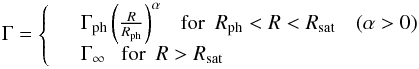
To estimate the photospheric radius we assume that most of the acceleration is completed
at Rph1. This is, for
example, the case in the simulations made by Tchekhovskoy
et al. (2010), where the Lorentz factor sharply increases beyond the stellar
radius, when the flow suddenly becomes unconfined. Then, in a first approximation, the
photospheric radius of a given shell writes (e.g. Piran
1999; Mészáros & Rees 2000; Daigne & Mochkovitch 2002)  (9)where
κ (κ0.2 in units of 0.2 cm2
g-1) is the material opacity and Γ (Γ2 in units of 100) the
Lorentz factor of the shell. The flow keeps a magnetisation σ at the end
of acceleration so that Ė/(1 + σ) is
the injected kinetic power ĖK. In the case of a passive
magnetic field that is carried by the outflow without contributing to its acceleration
(Spruit et al. 2001), the magnetisation
σ equals
(9)where
κ (κ0.2 in units of 0.2 cm2
g-1) is the material opacity and Γ (Γ2 in units of 100) the
Lorentz factor of the shell. The flow keeps a magnetisation σ at the end
of acceleration so that Ė/(1 + σ) is
the injected kinetic power ĖK. In the case of a passive
magnetic field that is carried by the outflow without contributing to its acceleration
(Spruit et al. 2001), the magnetisation
σ equals  (10)corresponding to a
pure and complete thermal acceleration. Efficient magnetic acceleration leads to
σ < σpassive,
whereas σ > σpassive
corresponds to an inefficient magnetic acceleration, for instance with no conversion of
magnetic into kinetic energy and some conversion of thermal into magnetic energy.
(10)corresponding to a
pure and complete thermal acceleration. Efficient magnetic acceleration leads to
σ < σpassive,
whereas σ > σpassive
corresponds to an inefficient magnetic acceleration, for instance with no conversion of
magnetic into kinetic energy and some conversion of thermal into magnetic energy.
When the shell reaches the photospheric radius, it releases its thermal energy content while a fraction of the remaining energy (kinetic or magnetic) can be dissipated farther away at a radius Rdiss by internal shocks for σ ≲ 0.1−1, or reconnection for higher magnetisation, contributing to the non-thermal emission of the burst. It is therefore expected, on theoretical grounds, that thermal and non-thermal components both contribute to the observed emission (Mészáros et al. 2002; Daigne & Mochkovitch 2002). As mentioned in the introduction, this was already supported by BATSE results, with new evidence now coming from Fermi (Guiriec et al. 2011; Zhang et al. 2011). In Sect. 3 we present synthetic bursts showing both contributions. We explain below our method to compute the thermal and non-thermal emission.
2.2. Thermal emission
The thermal emission can be computed from Eqs. (1), (2), (7), (8), and (9), for a given set of
central engine parameters ϵth, σ,
ℓ, θ, Ėiso, and a
distribution of the Lorentz factor in the flow. Both the thermal luminosity and observed
temperature are related to the injected power and temperature at the origin of the flow
via the same factor  (11)If a constant
Ėiso is assumed, the luminosity and temperature directly
trace the distribution of the Lorentz factor Γ(s), where the Lagrangian
coordinate s is the distance to the front of the flow at the end of the
acceleration stage (s/c is the
ejection time of the shell). The expanding flow becomes progressively transparent
(starting from the front) and the contribution of a shell located at s is
approximately received at an observer time
tobs = (1 + z)s/c
(Daigne & Mochkovitch 2002). However,
since the different parts of the flow do not become transparent at the same radius
(because Rph ∝ Γ-3), additional differences in
arrival time of the order of
(11)If a constant
Ėiso is assumed, the luminosity and temperature directly
trace the distribution of the Lorentz factor Γ(s), where the Lagrangian
coordinate s is the distance to the front of the flow at the end of the
acceleration stage (s/c is the
ejection time of the shell). The expanding flow becomes progressively transparent
(starting from the front) and the contribution of a shell located at s is
approximately received at an observer time
tobs = (1 + z)s/c
(Daigne & Mochkovitch 2002). However,
since the different parts of the flow do not become transparent at the same radius
(because Rph ∝ Γ-3), additional differences in
arrival time of the order of  (12)should be included. They
are, however, negligible as long as
Δtobs < tvar,
the typical variability time scale of the Lorentz factor.
(12)should be included. They
are, however, negligible as long as
Δtobs < tvar,
the typical variability time scale of the Lorentz factor.
The value of Δtobs also gives the time scale of the
luminosity decline after the last shell of the flow (emitted by the source at a time
τ) has reached the transparency radius (high-latitude emission). Unless
the Lorentz factor of this shell is small or the burst has a very short duration, the drop
in luminosity for
tobs > (1 + z)τ
is very steep, having initially a temporal decay index (see e.g. Sect. 6 in Beloborodov 2011)
 (13)This shows that in
models where the prompt emission comes from a Comptonised photosphere, the early decay of
index α ~ 3−5 observed in X-rays cannot be explained by the high
latitude emission and should instead be related to an effective decline of the central
engine (Hascoët et al. 2012).
(13)This shows that in
models where the prompt emission comes from a Comptonised photosphere, the early decay of
index α ~ 3−5 observed in X-rays cannot be explained by the high
latitude emission and should instead be related to an effective decline of the central
engine (Hascoët et al. 2012).
The expected count rate in a given spectral range and the resulting spectrum are obtained from the luminosity and temperature evolution (Eqs. (7) and (8)). However, we do not use a true Planck function for the elementary spectrum corresponding to a given temperature. As discussed in Goodman (1986) and Beloborodov (2010), geometrical effects at the photosphere lead to a low-energy spectral index close to α = +0.4 instead of α = +1 for a Raleigh-Jeans spectrum (see also Pe’er 2008). We therefore adopt a “modified Planck function” having the modified spectral slope at low energy, an exponential cutoff at high energy, peaking at ≃3.9 × kT as a Planck function in νFν, and carrying the same total energy.
2.3. Non-thermal emission
We first estimate the non-thermal emission assuming that it comes from internal shocks
(Rees & Meszaros 1994). For a given
distribution of the Lorentz factor, we obtain light curves and spectra using the
simplified model of Daigne & Mochkovitch
(1998), where the outflow is represented by a large number of shells that
interact by direct collisions only (see also Kobayashi et
al. 1997). The elementary spectrum for each collision is a broken power law with
the break at the synchrotron energy. The adopted values for the two spectral indices at
low and high energy respectively are α = −1 and
β = −2.25. The expected value for α in the fast
cooling regime should normally be −1.5 (see e.g. Sari et
al. 1998; Ghisellini et al. 2000), but
detailed radiative models including inverse Compton scattering in Klein-Nishina regime
tend to produce harder α slopes (Derishev
et al. 2001; Bošnjak et al. 2009; Nakar et al. 2009; Daigne et al. 2011), close to the typical observed value
α ≃ −1 (Preece et al. 2000;
Kaneko et al. 2006; Nava et al. 2011; Goldstein et al.
2012). The global efficiency of internal shocks is given by the product
 (14)where
fdiss is the efficiency for the dissipation of energy in
shocks and ϵe the fraction of the dissipated
energy transferred to electrons and eventually radiated. Typical values of
fIS do not exceed a few percents. We used this approach to
compute non-thermal light curves and spectra in Sect. 3.1 for the case of a low
magnetisation σ ≲ 0.1−1.
(14)where
fdiss is the efficiency for the dissipation of energy in
shocks and ϵe the fraction of the dissipated
energy transferred to electrons and eventually radiated. Typical values of
fIS do not exceed a few percents. We used this approach to
compute non-thermal light curves and spectra in Sect. 3.1 for the case of a low
magnetisation σ ≲ 0.1−1.
The presence of magnetic fields reduces shock efficiency and may even prevent shock
formation for σ ≳ 1 (Mimica &
Aloy 2010; Narayan et al. 2011). Then for
σ ≳ 1, the magnetic field cannot be ignored, and energy must be
extracted by magnetic reconnection (e.g. Thompson
1994; Spruit et al. 2001), possibly
triggered by internal shocks (Zhang & Yan
2011). Our limited understanding of the relevant processes does not allow a
reliable description of the resulting emission. Considering these difficulties, we have
adopted in Sect. 3.2 a very basic and simple point of view. We do not try to predict the
burst profile and obtain the spectrum in the following way: we suppose that a fraction
f Nth of the total injected energy eventually goes into
non-thermal emission with a spectrum represented by a Band function with low- and
high-energy spectral indices α = −1 and β = −2.25,
and a peak energy obtained from the Amati relation (Amati
et al. 2002) ![Mathematical equation: \begin{equation} \label{eqn_amati} E_{\rm p}\simeq 130\,\left[f_{\rm \,Nth}\,{E}_{\rm iso}\over 10^{52}\ {\rm erg}\right]^{0.55}\ \ {\rm keV} , \end{equation}](/articles/aa/full_html/2013/03/aa20023-12/aa20023-12-eq85.png) (15)where the exponent
and normalisation values are taken from Nava et al.
(2012). The validity of the Amati relation is strongly debated (see e.g. Nakar & Piran 2005; Band & Preece 2005; Kocevski
2012; Collazzi et al. 2012; Ghirlanda et al. 2012). It is not clear if it
corresponds to an intrinsic property of GRBs or if the relation results from a complex
chain of selection effects (threshold for burst detection, and various conditions for the
measure of the redshift and peak energy). For the purpose of the present study we do not
address this issue and use Eq. (15) simply
because it is approximately satisfied by the sample of long bursts for which the peak
energy and isotropic radiated energy have been measured.
(15)where the exponent
and normalisation values are taken from Nava et al.
(2012). The validity of the Amati relation is strongly debated (see e.g. Nakar & Piran 2005; Band & Preece 2005; Kocevski
2012; Collazzi et al. 2012; Ghirlanda et al. 2012). It is not clear if it
corresponds to an intrinsic property of GRBs or if the relation results from a complex
chain of selection effects (threshold for burst detection, and various conditions for the
measure of the redshift and peak energy). For the purpose of the present study we do not
address this issue and use Eq. (15) simply
because it is approximately satisfied by the sample of long bursts for which the peak
energy and isotropic radiated energy have been measured.
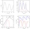 |
Fig. 2 Thermal and non-thermal emission from a variable outflow – internal shock framework. Top left: initial distribution of the Lorentz factor in the flow. Top right: thermal (red), non-thermal (blue), and total (black) photon flux in the 8 keV–40 MeV spectral range. Bottom left: thermal (red), non-thermal (blue), and total (black) time-integrated spectra. Bottom right: instant temperature (red) of the photospheric emission and instant peak energy (blue) of the internal shock emission. The dotted and dashed lines correspond to the temperature and peak energy averaged over time intervals of 2 and 4 s, respectively. The adopted flow parameters are Ėiso = 1053 erg s-1, ϵth = 0.03, σ = 0.1, ℓ = 3 × 106 cm, and θ = 0.1 rad; a redshift z = 1 is assumed. |
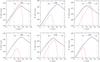 |
Fig. 3 Thermal and non-thermal emission from a variable outflow – internal shock framework: impact of the outflow parameters. Starting from the reference case shown in Fig. 2 (with a redshift z = 1) we first change the thermal fraction ϵth to 0.3 (top left panel) and 0.003 (bottom left); then the isotropic power Ėiso to 1054 erg s-1 (top middle) and 1052 erg s-1 (bottom middle); and finally the Lorentz factor is multiplied (top right) and divided (bottom right) by a factor of 2. Each time we vary a parameter, all the others keep the value corresponding to the reference case. |
3. Results
3.1. Non-thermal emission from internal shocks
To study the relative intensities of the thermal and non-thermal emission components we
have considered as an example a flow ejected by a central source active for a duration
stot/c = 10 s, where the
Lorentz factor takes the form ![Mathematical equation: \begin{equation} \label{eqn_gp_complex} \Gamma(s)=333 \left\lbrace 1+\frac{2}{3} \ {\rm cos}\left[5\,\pi \left( 1-{s\over s_{\rm tot}}\right)\right]\,\right\rbrace\times \exp{\left(-{s\over 2 s_{\rm tot}}\right)} \cdot \end{equation}](/articles/aa/full_html/2013/03/aa20023-12/aa20023-12-eq98.png) (16)This distribution is
arbitrary (see other possible examples in Daigne &
Mochkovitch 1998) and was adopted simply to produce a burst made of three pulses,
i.e. not too simple and not too complex. It is is shown in Fig. 2 (top left panel) together with the non-thermal light curve (between 8
keV and 40 MeV; top right panel) resulting from internal shocks. The related photospheric
emission is shown in the same energy range for ϵth = 0.03. We
adopt a constant Ėiso = 1053 erg s-1,
σ = 0.1, ℓ = 3 × 106 cm and
θ = 0.1 rad (i.e.
l/θ = 300 km). We also represent in
the bottom left and bottom right panels the spectrum (thermal, non-thermal, and global)
and the temporal evolution of the instantaneous peak energy and temperature of the
non-thermal and thermal emissions. As the thermal spectrum is a superposition of
elementary modified Planck functions at different temperatures, its average spectral slope
α (with
N(E) ∝ Eα)
below the peak is close to −1. The asymptotic value α = +0.4 is
recovered only below a few keV, which corresponds to the photospheric contribution with
the lowest temperature.
(16)This distribution is
arbitrary (see other possible examples in Daigne &
Mochkovitch 1998) and was adopted simply to produce a burst made of three pulses,
i.e. not too simple and not too complex. It is is shown in Fig. 2 (top left panel) together with the non-thermal light curve (between 8
keV and 40 MeV; top right panel) resulting from internal shocks. The related photospheric
emission is shown in the same energy range for ϵth = 0.03. We
adopt a constant Ėiso = 1053 erg s-1,
σ = 0.1, ℓ = 3 × 106 cm and
θ = 0.1 rad (i.e.
l/θ = 300 km). We also represent in
the bottom left and bottom right panels the spectrum (thermal, non-thermal, and global)
and the temporal evolution of the instantaneous peak energy and temperature of the
non-thermal and thermal emissions. As the thermal spectrum is a superposition of
elementary modified Planck functions at different temperatures, its average spectral slope
α (with
N(E) ∝ Eα)
below the peak is close to −1. The asymptotic value α = +0.4 is
recovered only below a few keV, which corresponds to the photospheric contribution with
the lowest temperature.
It can be seen in Fig. 2 (top right panel) that the
emission is initially only thermal as it takes a time  (17)for the first signal from
internal shocks to arrive at the observer. In Eq. (17) the subscript “0” refers to the radius and Lorentz factor of the
first shocked shell that contributes to the non-thermal emission. At late times the
situation is just the opposite: the photospheric emission abruptly stops at
tobs = 20 s, while the emission from late internal shocks
(both on- and off-axis) still contribute for about 10 s (observer frame). The spectrum
(Fig. 2, bottom left) is the sum of the thermal and
non-thermal contributions. They peak at 200/(1 + z)
and 1000/(1 + z) keV, respectively. Finally the plot
of the temperature and of the peak energy of the non-thermal spectrum as a function of
observer time shows (Fig. 2, bottom right panel) that
the former is more sensitive than the latter to the fluctuations of the Lorentz factor
(since Tobs ∝ Γ8/3).
(17)for the first signal from
internal shocks to arrive at the observer. In Eq. (17) the subscript “0” refers to the radius and Lorentz factor of the
first shocked shell that contributes to the non-thermal emission. At late times the
situation is just the opposite: the photospheric emission abruptly stops at
tobs = 20 s, while the emission from late internal shocks
(both on- and off-axis) still contribute for about 10 s (observer frame). The spectrum
(Fig. 2, bottom left) is the sum of the thermal and
non-thermal contributions. They peak at 200/(1 + z)
and 1000/(1 + z) keV, respectively. Finally the plot
of the temperature and of the peak energy of the non-thermal spectrum as a function of
observer time shows (Fig. 2, bottom right panel) that
the former is more sensitive than the latter to the fluctuations of the Lorentz factor
(since Tobs ∝ Γ8/3).
We now check how these results change when we vary the model parameters. We divide these
parameters into three groups describing respectively the geometry (θ,
l); the energetics and flow-acceleration mechanism
(Ėisoϵth, σ);
and the ejecta structure (stot,
 ,
,
 ),
where
and
),
where
and  are the contrast (
 )
and average of the Lorentz factor distribution.
)
and average of the Lorentz factor distribution.
The geometry only affects the thermal emission (for a fixed Ėiso). The dependence of Tobs and Lth, iso on θ and ℓ is weak. From Eqs. (2), (7), and (8) we get Tobs ∝ θ−1/6ℓ1/6 and Lth, iso ∝ θ−2/3ℓ2/3. Similarly, changing the magnetisation has a moderate effect on the previous results, as long as σ < 1. As explained above, for σ ≳ 1 the whole theoretical framework adopted to compute the non-thermal emission probably becomes invalid.
The consequence of increasing or decreasing the thermal fraction ϵth is illustrated in Fig. 3 (left panels). With ϵth = 0.3 the thermal spectrum overtakes the non-thermal spectrum between 20/(1 + z) and 500/(1 + z) keV, and the thermal component represents about one third of the total in the light curve. Conversely, with ϵth = 0.003 the contribution of the thermal component to the global spectrum and the light curve is barely visible.
The dependence of the temperature and thermal luminosity on the injected isotropic power
Ėiso and average Lorentz factor
can be also obtained from Eqs. (2), (7), and (8) yielding ![Mathematical equation: \begin{eqnarray} \label{eqn_tobs_depend} &T_{\rm obs} \propto {\dot E}_{\rm iso}^{-5/12}\,{\bar \Gamma}^{8/3} , \\[4mm] \label{eqn_lth_depend} &L_{\rm th, \,iso} \propto {\dot E}_{\rm iso}^{1/3}\,{\bar \Gamma}^{8/3} . \end{eqnarray}](/articles/aa/full_html/2013/03/aa20023-12/aa20023-12-eq125.png) For
the non-thermal component, the relation of the peak energy and luminosity to the model
parameters can be found using the simplest possible description of internal shocks that
only considers the interaction of two shells of equal mass (Barraud et al. 2005). One gets
For
the non-thermal component, the relation of the peak energy and luminosity to the model
parameters can be found using the simplest possible description of internal shocks that
only considers the interaction of two shells of equal mass (Barraud et al. 2005). One gets ![Mathematical equation: \begin{eqnarray} &E_{\rm p} \propto \dot{E}_{\rm K}^{1/2}\varphi({\cal C})\, \bar{\Gamma}^{-2}\ t_{\rm var}^{-1} , \\[4mm] &L_{\rm Nth, \,iso} \propto f_{\rm IS}\,{\dot E}_{\rm iso} , \end{eqnarray}](/articles/aa/full_html/2013/03/aa20023-12/aa20023-12-eq126.png) where
tvar is of the order of one pulse duration,
where
tvar is of the order of one pulse duration,
 depends on
only, and fIS, defined by Eq. (14), is given by
depends on
only, and fIS, defined by Eq. (14), is given by  (22)It can be seen that the
thermal and non-thermal components behave quite differently when the injected power and
average Lorentz factor are changed. This is illustrated in Fig. 3 where we increase or decrease Ėiso and
by respective factors of 10 and 2, compared to the reference case shown in Fig. 2.
(22)It can be seen that the
thermal and non-thermal components behave quite differently when the injected power and
average Lorentz factor are changed. This is illustrated in Fig. 3 where we increase or decrease Ėiso and
by respective factors of 10 and 2, compared to the reference case shown in Fig. 2.
It appears that for a given value of ϵth
(ϵth = 0.03 in Fig. 3,
middle and right panels) the thermal component becomes more visible when
Ėiso is decreased and
increased. This is a direct consequence of Eqs. (18) and (19) above, which can be
made even more explicit by defining the global thermal efficiency (assuming
κ = 0.2 cm2 g-1)  (23)to be compared to
the non-thermal efficiency
fNth = fIS approximated by Eq.
(22). While changing
Ėiso and
affects only the thermal efficiency, the opposite is true for the contrast in Lorentz
factor .
Reducing
makes internal shocks much less efficient and considerably softens the emitted non-thermal
spectrum. In the limit where
(23)to be compared to
the non-thermal efficiency
fNth = fIS approximated by Eq.
(22). While changing
Ėiso and
affects only the thermal efficiency, the opposite is true for the contrast in Lorentz
factor .
Reducing
makes internal shocks much less efficient and considerably softens the emitted non-thermal
spectrum. In the limit where  (and moreover if the Lorentz factor is increasing outwards in the ejecta) there will be no
internal shocks and the emission will only be thermal in the absence of an alternative
dissipation process.
(and moreover if the Lorentz factor is increasing outwards in the ejecta) there will be no
internal shocks and the emission will only be thermal in the absence of an alternative
dissipation process.
3.2. Non-thermal emission from magnetic dissipation
If the non-thermal emission is produced by reconnection in a magnetised outflow, the problem becomes very difficult, with no simple way to accurately follow the process in time and compute a light curve (see e.g. Spruit et al. 2001; Lyutikov & Blandford 2003; Giannios 2008; Zhang & Yan 2011; McKinney & Uzdensky 2012). As explained in Sect. 2.3 above, we adopted a very simple assumption to obtain the non-thermal spectrum: a Band function carrying a fraction fNth of the injected energy with the peak of E2N(E) obtained from the Amati relation. Several examples of the thermal and non-thermal spectra are represented in the left panel of Fig. 4, with the thermal component still being computed with the distribution of Lorentz factor given by Eq. (16). The results are shown for several values of ϵth and σ, and a fixed value of the isotropic magnetic power at the photosphere σĖ/(1 + σ) = 1053 erg s-1. As expected, the detection of the photospheric component in the spectrum is favored by a high ϵth, a low fNth, and a high Γ. The specific dependency on the magnetisation is discussed in the next section.
 |
Fig. 4 Thermal and non-thermal emission from a variable outflow – magnetic reconnection framework. In each panel we show a sequence of thermal (red) and non-thermal (blue), spectra (the source redshift is z = 1). The Lorentz factor distribution adopted for the calculation of the thermal emission is the same as in Fig. 2 (left panel) or the same but with Γ divided by 2 (right panel). The thermal emission is computed using the formalism developed in Sect. 2.2, using five values of ϵth: 0.01, 0.03, 0.10, 0.30, and 0.5. The non-thermal spectrum is simply parametrised by a Band function, with the peak energy being given by the Amati relation (see text) and using five values of the efficiency of the magnetic reconnection, frec = fNth(1 + σ)/σ: 0.01, 0.03, 0.10, 0.30, and 0.5. In all cases, the isotropic magnetic power at the photosphere is fixed to σĖiso/(1 + σ) = 1053 erg s-1. Finally, the magnetisation σ at large distance is either σ = 1 (solid lines) or 10 (dashed lines). |
4. Discussion
4.1. Relative intensity of the thermal component in GRBs
Depending on the mechanism responsible for the acceleration of the outflow in GRBs, the consequences regarding the photospheric emission are very different. In a pure fireball (ϵth = 1) powered by neutrino-antineutrino annihilation (see e.g. Popham et al. 1999; Zalamea & Beloborodov 2011), the predicted thermal emission is very bright (Daigne & Mochkovitch 2002). To agree with the current data, the spectrum should then be Comptonised at high energy (as a result of some dissipative process below the photosphere, e.g. Rees & Mészáros 2005; Pe’er et al. 2006; Giannios 2008; Beloborodov 2010; Lazzati & Begelman 2010) to produce a power law tail and softened at low energy to decrease the spectral index α from a positive value to a negative one (possibly by the presence of an additional non-thermal component, e.g. Pe’er et al. 2006; Vurm et al. 2011). An alternative is to suppose that the flow is initially magnetically dominated (ϵth ≲ 0.1). A thermal component is still expected to be released at the photosphere, but it will now be sub-dominant compared to non-thermal processes such as internal shocks or magnetic reconnection.
We have explored this second possibility in the present paper, making the following assumptions: (i) we supposed that the flow evolves adiabatically from the origin to the photosphere, i.e. we did not include possible sources of heating below Rph; (ii) if the remaining magnetisation σ at the end of acceleration is weak and does not prevent the formation of internal shocks, we computed their contribution to the emitted radiation as if σ = 0; (iii) when σ > 1 we limited ourselves to a very simple parametrised study where we assumed that a fraction fNth of the injected power goes into the non-thermal component.
Regarding the light curve and spectrum of the thermal emission we obtained the following results:
-
Both the photosphere luminosity and temperature depend on thesame factor Φ given by Eq. (11), which directly traces the evolution of the Lorentz factor if the injected power stays constant.
-
The duration of the photospheric emission corresponds to the duration τ of production of the relativistic wind. For t > τ the luminosity drops rapidly on a time scale
 a
few ms for typical values of the burst parameters.
a
few ms for typical values of the burst parameters. -
The global spectrum of the thermal emission is a composite of many elementary contributions at different temperatures. Before asymptotically reaching a slope α = +0.4 at low energy it can be much softer below the peak as shown in Fig. 2. A time resolved spectrum will resemble more closely the “modified Planck function” adopted for each elementary collision.
If the non-thermal emission comes from internal shocks, its light curve and spectrum have
been computed using the simplified approach described in Sect. 2.3. We have varied several of the model parameters: fraction
ϵth of thermal energy at the origin of the flow, isotropic
injected power Ėiso, and average
to see under which conditions the thermal component would appear in the observed spectrum,
in the internal shock scenario for σ ≲ 0.1−1 (Fig. 3) or in the magnetic reconnection scenario for σ ≳ 1
(Fig. 4). In the internal shock framework, assuming
κ = 0.2 cm2 g-1, the ratio Q
of the thermal to non-thermal efficiency is given by  (24)As illustrated by
this formula and in Fig. 3, increasing
ϵth, but also increasing
or reducing Ėiso or
(24)As illustrated by
this formula and in Fig. 3, increasing
ϵth, but also increasing
or reducing Ėiso or  will make the thermal component more visible. The magnetisation σ has a
low impact as 1 + σ ≃ 1 in this scenario. In the examples shown in Fig.
3, the model parameters are taken from the
reference case used in Fig. 2 and equal
l7 = 0.3, θ-1 = 1,
ϵe = 1/3, and
σ = 0.1. The effective constrast corresponding to the initial
distribution of the Lorentz factor plotted in the upper left panel of Fig. 2 is
will make the thermal component more visible. The magnetisation σ has a
low impact as 1 + σ ≃ 1 in this scenario. In the examples shown in Fig.
3, the model parameters are taken from the
reference case used in Fig. 2 and equal
l7 = 0.3, θ-1 = 1,
ϵe = 1/3, and
σ = 0.1. The effective constrast corresponding to the initial
distribution of the Lorentz factor plotted in the upper left panel of Fig. 2 is  .
Then Eq. (24) leads to
.
Then Eq. (24) leads to
 ,
in reasonable agreement with Fig. 3: for instance,
the upper left panel corresponds to ϵth = 0.3,
Ėiso,53 = 1,
,
in reasonable agreement with Fig. 3: for instance,
the upper left panel corresponds to ϵth = 0.3,
Ėiso,53 = 1,
 ,
and Q ≃ 0.4, and the bottom right panel corresponds to
ϵth = 0.03,
Ėiso,53 = 1,
,
and Q ≃ 0.4, and the bottom right panel corresponds to
ϵth = 0.03,
Ėiso,53 = 1,
 ,
and Q ≃ 0.006. Note that in the
E2N(E) spectrum, the ratio
of the maxima of the two components is expected to be slightly higher than
Q because the photospheric component has a narrower spectrum than the
non-thermal one.
,
and Q ≃ 0.006. Note that in the
E2N(E) spectrum, the ratio
of the maxima of the two components is expected to be slightly higher than
Q because the photospheric component has a narrower spectrum than the
non-thermal one.
In the case of magnetic reconnection, the non-thermal emission is simply parametrised by
its global efficiency fNth, and we have  (25)in good agreement with
Fig. 4
(fNth, −2 being the non-thermal efficiency
in %). Especially, Eq. (25) shows that the
ratio Q increases with the magnetisation σ, which seems
counter-intuitive. For a fixed value of Ė, increasing σ
reduces ĖK, and therefore decreases the photospheric radius
Rph (see Eq. (9)). Therefore, for a given value of ϵth, the
luminosity and temperature of the photosphere increase. However, for a given acceleration
mechanism, one would expect an increase of σ to be associated with a
decrease of ϵth, which may affect the dependency of the ratio
Q on the magnetisation σ. For instance, in the case of
a passive magnetic field, including
σ = σpassive in Eq. (25) leads to
(25)in good agreement with
Fig. 4
(fNth, −2 being the non-thermal efficiency
in %). Especially, Eq. (25) shows that the
ratio Q increases with the magnetisation σ, which seems
counter-intuitive. For a fixed value of Ė, increasing σ
reduces ĖK, and therefore decreases the photospheric radius
Rph (see Eq. (9)). Therefore, for a given value of ϵth, the
luminosity and temperature of the photosphere increase. However, for a given acceleration
mechanism, one would expect an increase of σ to be associated with a
decrease of ϵth, which may affect the dependency of the ratio
Q on the magnetisation σ. For instance, in the case of
a passive magnetic field, including
σ = σpassive in Eq. (25) leads to
 ,
i.e. a decreasing ratio for an increasing magnetisation. Since increasing the final
magnetisation σ tends to decrease the photospheric radius, it should also
be noted that the acceleration of the flow may well be incomplete at the photosphere in
high σ scenarios. As discussed in Appendix A, this will also reduce the photospheric emission.
,
i.e. a decreasing ratio for an increasing magnetisation. Since increasing the final
magnetisation σ tends to decrease the photospheric radius, it should also
be noted that the acceleration of the flow may well be incomplete at the photosphere in
high σ scenarios. As discussed in Appendix A, this will also reduce the photospheric emission.
4.2. Comparison to observations
We now check how these results compare to the various observational indications of the presence of a thermal component in GRB spectra.
One first indirect indication comes from the very hard spectral slopes
α > 0 that are sometimes observed during burst
evolution (e.g. Ghirlanda et al. 2003; Bosnjak et al. 2006; Abdo
et al. 2009). Indeed, our results allow the thermal over non-thermal ratio (Eq.
(24)) to vary with time. A locally large
will boost the thermal component while a low contrast
will reduce the non-thermal component (under the condition that the non-thermal emission
comes from internal shocks). This can explain an erratic behaviour of the
α slope, but observations often show a regular shift of
α from positive to negative values during a single pulse. As explained
in Sect. 3.1 a thermal start and a non-thermal ending are predicted by our models, but the
fraction of time during which the emission is thermal is generally smaller than observed
in the few bursts where the measured α slope is positive. It remains
possible to adopt a distribution of the Lorentz factor that would extend the duration of
the thermal emission but smoothly connecting the thermal and non-thermal components may
not be easy.
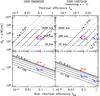 |
Fig. 5 Constraints on the thermal and non-thermal emission in GRB 090902B and GRB 100724B. Top: for a given thermal fraction ϵth = 10-2, 10-1.5, 10-1, 10-0.5, and 1, the radius R0 = ℓ/θ at the base of the flow is plotted as a function of the non-thermal efficiency fNth. The corresponding thermal efficiency fth is also shown (top x-axis). Bottom: for a given magnetisation σ = 10-1, 10-0.5, 1, 100.5, 101, 101.5, and 102 at the end of acceleration phase, the Lorentz factor of the flow is plotted as a function of fNth (the unmagnetised case σ = 0 cannot be distinguished from the case σ = 0.1). Sets of parameters representative of the different classes of scenarios discussed in the paper are indicated: F (ϵth = 1, σ = 0) (standard fireball), M,is1 (log ϵth = −0.5, σ = 0,) and M,is2 (log ϵth = −1.5, σ = 0) (efficient magnetic acceleration: magnetisation is low above the photosphere and the dominant non-thermal mechanism is internal shocks), M,rec1 (log ϵth = −0.5, σ = 10), and M,rec2 (log ϵth = −1.5, σ = 10) (magnetised flow at large distance, the dominant non-thermal mechanism is magnetic reconnection). The initial radius is fixed to R0 = 300 km, a typical value for long GRBs. The observational data (thermal flux, temperature, ratio of the thermal over the total flux) used for the calculation (see text) are taken from Abdo et al. (2009); Pe’er et al. (2012) for GRB 090902B (left column), and from Guiriec et al. (2011) for GRB 100724B (right column). |
A second indication comes from the recent detection of possible thermal components in a few Fermi GRBs. GRB 090902B is a very peculiar case of a burst showing a spectrum best fitted by a Band function with a hard low-energy photon index, or a multi-colour black body, together with an additional sub-dominant power law (Abdo et al. 2009; Ryde et al. 2010). A first possibility is to interpret this burst as photospheric emission with additional dissipative processes affecting the spectrum by Comptonisation and possibly other non-thermal processes. Conversely, using the formalism presented here, we can also derive constraints on the burst parameters for alternative scenarios where the Band component is interpreted as the thermal emission produced at the photosphere without sub-photospheric dissipation, and the power law as non-thermal emission produced above the photosphere in the optically thin regime. From the analysis made by Abdo et al. (2009) and Pe’er et al. (2012), the implied thermal luminosity and temperature are large, Lth ≃ 4.6 × 1053 erg s-1 and Tobs ≃ 168 keV. The thermal luminosity represents 53% of the total luminosity. Then, for a given ϵth, σ, and fNth, one can deduce from Eqs. (7)–(9) the isotropic power Ėiso, the size R0 = ℓ/θ of the region at the base of the outflow (see Fig. 5, top-left panel), and the Lorentz factor Γ (see Fig. 5, bottom-left panel). This is a similar approach to the one proposed by Pe’er et al. (2007), but within the more general framework defined in this paper, which allows us to consider several scenarios for the acceleration of the outflow. As GRB 090902B is very bright, this leads to huge values of Ėiso, the minimum being obtained for ϵth ≃ 1, which would make GRB 090902B a peculiar burst associated to a situation close to a pure fireball. For instance, for ϵth = 1, l7 = 0.3, θ-1 = 1 (i.e. R0 = 300 km), and σ ≪ 1 we get an isotropic power Ėiso ~ 2.6 × 1054 erg s-1 and a Lorentz factor Γ ~ 1160. The efficiency of the photospheric emission in this case is fth ≃ 0.18 and the efficiency of the non-thermal emission above the photosphere is fNth ≃ 0.16, marginally compatible with internal shocks. This case is labelled as F in Fig. 5 (left column) and is in good agreement with the analysis made by Pe’er et al. (2012).
As most GRBs do not show such a bright thermal component, they usually require much lower values of ϵth, as illustrated below with GRB 100724B. Then, it is worth studying the possibility to model GRB 090902B with ϵth < 1, which would correspond to an initially magnetised outflow. Reducing ϵth in this burst has several consequences. As illustrated in Fig. 5 (left column), it implies a general decrease of the efficiency, except if the initial size R0 = ℓ/θ is very large (R0 ≫ 3000 km), which is not expected for most models of the central engine of long GRBs, because of their short timescale (~1–10 ms) variability. For instance, for ϵth = 10-0.5 (case labelled as M,is1, where we keep R0 = 300 km and σ ≪ 1), the thermal and non-thermal efficiencies are reduced to fth = 0.06 and fNth = 0.05, leading to an isotropic equivalent power Ėiso = 9.4 × 1054 erg s-1. It also leads to an increase of the Lorentz factor, which was already quite high for the pure fireball scenario (see Fig. 5, bottom-left panel). Therefore, ϵth ≃ 0.3−0.5 seems a reasonable lower limit for GRB 090902B. Note that a decrease of ϵth compared to the standard fireball leads in this case to a reduced non-thermal efficiency fth in good agreement with the expected value for internal shocks. For higher values of ϵth, magnetic reconnection, which is supposed to have a higher efficiency, is a better candidate, as illustrated in Fig. 5 (left column). In addition, for a fixed value of ϵth, increasing the magnetisation σ at the end of acceleration always reduces the constraint on the Lorentz factor (bottom left panel). A more detailed modelling of GRB 090902B would be necessary to distinguish between these different possibilities.
Conversely, the results of Guiriec et al. (2011) indicating the presence of a sub-dominant thermal component in GRB 100724B, representing about 4% of the total flux, point towards low values of ϵth and, therefore, a magnetic acceleration. As shown in Fig. 5, it is difficult to interpret GRB 100724B within the standard fireball scenario (thermal acceleration) that would imply either fNth > 1 or R0 < 120 km (and even R0 < 40 km if fNth < 0.5 is required). This is obtained assuming a redshift z = 1, but we checked that our conclusions are unchanged for larger redshifts. Then a low thermal fraction ϵth ≲ 0.01−0.1 is required in GRB 100724B, whose spectral properties are much more representative of the bulk GRB population than in the unusual case of GRB 090902B. A similar conclusion was obtained by Zhang & Pe’er (2009) in the case of the very energetic burst GRB 080916C where no bright thermal component was detected. Assuming a passive magnetic field below the photosphere, they obtain the constraint σpassive ≳ 15−20, which leads to the more general condition ϵth ≲ 0.05, from Eq. (10).
If magnetic acceleration is common in GRBs, several scenarios can be discussed. In scenarios where magnetic acceleration is efficient, implying a low magnetisation at large radius and a dominant role of internal shocks, the thermal fraction should not be much larger than a few percents to avoid an unrealistic efficiency fNth. For instance in the case of GRB 100724B, for z = 1, ϵth = 10-1.5, ℓ7 = 0.3, θ-1 = 1 (i.e. R0 = 300 km), and σ ≪ 1 (case labelled as M,is2 in Fig. 5 right column), we get a non-thermal efficiency fNth ≃ 0.06 and a thermal efficiency fth ≃ 2 × 10⁻³. The isotropic kinetic power and the Lorentz factor in this case are Ėiso ≃ 5.6 × 1053 erg s-1 and Γ ≃ 660. Alternative scenarios – where the flow is still magnetised at large radius and magnetic reconnection is the dominant mechanism to produce non-thermal emission – are less constrained, because of the uncertainties in the underlying physics. As illustrated in Fig. 5, for a fixed ϵth, increasing σ tends to reduce Γ, which is already in the typical range of a few hundreds for σ = 0. High values of the non-thermal efficiency fNth ≳ 0.1−0.5 (as usually expected for magnetic reconnection, see e.g. Zhang & Yan 2011; McKinney & Uzdensky 2012) also require high values of the thermal fraction ϵth ≳ 0.1−0.3, which does not seem natural in such scenarios of highly magnetised outflows.
As illustrated in Sect. 3, spectra with non-thermal and thermal components resembling those found by Guiriec et al. (2011) are easily obtained with our model, either for a photospheric + internal shocks scenario in a case of efficient magnetic acceleration, or for a photospheric + reconnection scenario if the magnetisation at large distance is still large. A potential issue for the internal shock scenario is the moderate variation of the temperature (within a factor of 2) found in the time-resolved analysis. To be efficient, internal shocks require large fluctuations of the Lorentz factors that are even amplified in the observed temperature (Tobs ∝ Γ8/3, see Fig. 2). This may suggest that the non-thermal emission in GRB 100724B comes from magnetic reconnection. This is unfortunately difficult to test in absence of theoretical predictions for the spectral evolution in this case. It should however be noted that when the temperature drops, the luminosity also drops so that, in practice, the temperature can be determined only when it is high enough. Depending on the time scale for the Lorentz factor fluctuations and the temporal resolution of the analysis, this may artificially reduce the amplitude of the measured variations of temperature. This is illustrated in Fig. 2 where dotted and dashed lines show the temperature (and peak energy of the non-thermal spectrum) averaged over intervals of 2 and 4 s, respectively. It remains to be tested if this smoothing effect can account for GRB 100724B evolution in the photospheric + internal shocks scenario.
5. Conclusion
We have explored in detail GRB scenarios with two episodes of emission: thermal emission from the photosphere without sub-photospheric dissipation, and non-thermal emission from internal dissipation above the photosphere. Our results can be used to interpret the data and obtain constraints on the burst parameters or acceleration mechanism. But one faces the difficulty arising from the diversity of the proposed evidence for the presence of a thermal component in GRB spectra. In some cases this thermal component represents a major contribution to the global spectrum (with additional non-thermal contributions) while in others it is always sub-dominant, most of the emission having a non-thermal origin. These different situations seem to imply quite different magnetic over thermal energy ratios at the origin of the flow. However the lack of bright thermal components in most GRBs clearly points towards magnetic acceleration, with ϵth ≲ 0.01 in most cases, and ϵth ≃ 0.01−0.1 in less frequent cases such as GRB 100724B. GRB 090902B with ϵth ≃ 0.3−1 remains an exception2.
More generally, one may wonder what would be the best conditions for the thermal emission
to show up. Apart from the obvious requirement that ϵth should
be as large as possible, Eq. (24) may
suggest looking for events with a low Ėiso and/or a large
average Lorentz factor. This, however, supposes that these two quantities are independent.
Having  and q > 1/4 would favor both a
large Ėiso and Γ while the opposite is true for
q < 1/4. Finally, if the
non-thermal emission comes from internal shocks, a pure thermal spectrum can be possible
even if the distribution of the Lorentz factor has a low contrast or if Γ is increasing
outwards.
and q > 1/4 would favor both a
large Ėiso and Γ while the opposite is true for
q < 1/4. Finally, if the
non-thermal emission comes from internal shocks, a pure thermal spectrum can be possible
even if the distribution of the Lorentz factor has a low contrast or if Γ is increasing
outwards.
The observation of a burst with an unambiguous photospheric signature in its spectrum would greatly help to clarify several issues in GRB physics: (i) estimating the value of ϵth would provide insight on the acceleration mechanism of the flow; (ii) obtaining the temperature and thermal luminosity evolution would constrain the distribution of Lorentz factor and injected power; and (iii) measuring the level of temperature fluctuations with a high temporal resolution would help to discriminate between internal shocks and magnetic reconnection for the non-thermal emission. Isolating the photospheric component in the available data is, however, not an easy task: it is generally one among other spectral components and possibly sub-dominant, and does not have a simple blackbody spectrum.
See Appendix A for a short discussion of the case where Rsat > Rph.
An intermediate case between GRB 100724B and 090902B has been recently found in the short GRB 120323A (Guiriec et al. 2012).
Acknowledgments
The authors thank the referee for constructive comments helping us to clarify the formulation of the paper. This work is partially supported by a grant from the French Space Agency (CNES). R.H.’s PhD work is funded by a Fondation CFM-JP Aguilar grant.
References
- Abdo, A. A., Ackermann, M., Ajello, M., et al. 2009, ApJ, 706, L138 [NASA ADS] [CrossRef] [Google Scholar]
- Amati, L., Frontera, F., Tavani, M., et al. 2002, A&A, 390, 81 [NASA ADS] [CrossRef] [EDP Sciences] [Google Scholar]
- Band, D. L., & Preece, R. D. 2005, ApJ, 627, 319 [NASA ADS] [CrossRef] [Google Scholar]
- Band, D., Matteson, J., Ford, L., et al. 1993, ApJ, 413, 281 [NASA ADS] [CrossRef] [Google Scholar]
- Barraud, C., Daigne, F., Mochkovitch, R., & Atteia, J. L. 2005, A&A, 440, 809 [NASA ADS] [CrossRef] [EDP Sciences] [Google Scholar]
- Begelman, M. C., & Li, Z.-Y. 1994, ApJ, 426, 269 [NASA ADS] [CrossRef] [Google Scholar]
- Beloborodov, A. M. 2010, MNRAS, 407, 1033 [NASA ADS] [CrossRef] [Google Scholar]
- Beloborodov, A. M. 2011, ApJ, 737, 68 [NASA ADS] [CrossRef] [Google Scholar]
- Bosnjak, Z., Celotti, A., & Ghirlanda, G. 2006, MNRAS, 370, L33 [NASA ADS] [CrossRef] [Google Scholar]
- Bošnjak, Ž., Daigne, F., & Dubus, G. 2009, A&A, 498, 677 [NASA ADS] [CrossRef] [EDP Sciences] [Google Scholar]
- Brainerd, J. J., & Lamb, D. Q. 1987, ApJ, 313, 231 [NASA ADS] [CrossRef] [Google Scholar]
- Cline, T. L., & Desai, U. D. 1975, ApJ, 196, L43 [NASA ADS] [CrossRef] [Google Scholar]
- Cline, T. L., Desai, U. D., Klebesadel, R. W., & Strong, I. B. 1973, ApJ, 185, L1 [NASA ADS] [CrossRef] [Google Scholar]
- Collazzi, A. C., Schaefer, B. E., Goldstein, A., & Preece, R. D. 2012, ApJ, 747, 39 [NASA ADS] [CrossRef] [Google Scholar]
- Daigne, F., & Drenkhahn, G. 2002, A&A, 381, 1066 [NASA ADS] [CrossRef] [EDP Sciences] [Google Scholar]
- Daigne, F., & Mochkovitch, R. 1998, MNRAS, 296, 275 [NASA ADS] [CrossRef] [Google Scholar]
- Daigne, F., & Mochkovitch, R. 2002, MNRAS, 336, 1271 [NASA ADS] [CrossRef] [Google Scholar]
- Daigne, F., Bošnjak, Ž., & Dubus, G. 2011, A&A, 526, A110 [NASA ADS] [CrossRef] [EDP Sciences] [Google Scholar]
- Derishev, E. V., Kocharovsky, V. V., & Kocharovsky, V. V. 2001, A&A, 372, 1071 [NASA ADS] [CrossRef] [EDP Sciences] [Google Scholar]
- Ghirlanda, G., Celotti, A., & Ghisellini, G. 2003, A&A, 406, 879 [NASA ADS] [CrossRef] [EDP Sciences] [Google Scholar]
- Ghirlanda, G., Ghisellini, G., Nava, L., et al. 2012, MNRAS, 422, 2553 [NASA ADS] [CrossRef] [Google Scholar]
- Ghisellini, G., Celotti, A., & Lazzati, D. 2000, MNRAS, 313, L1 [NASA ADS] [CrossRef] [Google Scholar]
- Giannios, D. 2008, A&A, 480, 305 [NASA ADS] [CrossRef] [EDP Sciences] [Google Scholar]
- Giannios, D. 2012, MNRAS, 422, 3092 [NASA ADS] [CrossRef] [Google Scholar]
- Giannios, D., & Spruit, H. C. 2007, A&A, 469, 1 [NASA ADS] [CrossRef] [EDP Sciences] [Google Scholar]
- Gilman, D., Metzger, A. E., Parker, R. H., Evans, L. G., & Trombka, J. I. 1980, ApJ, 236, 951 [Google Scholar]
- Goldstein, A., Burgess, J. M., Preece, R. D., et al. 2012, ApJS, 199, 19 [NASA ADS] [CrossRef] [Google Scholar]
- Goodman, J. 1986, ApJ, 308, L47 [NASA ADS] [CrossRef] [Google Scholar]
- Granot, J., Komissarov, S. S., & Spitkovsky, A. 2011, MNRAS, 411, 1323 [Google Scholar]
- Guiriec, S., Connaughton, V., Briggs, M. S., et al. 2011, ApJ, 727, L33 [NASA ADS] [CrossRef] [Google Scholar]
- Guiriec, S., Daigne, F., Hascoët, R., et al. 2012, ApJ, submitted [arXiv:1210.7252] [Google Scholar]
- Hascoët, R., Daigne, F., & Mochkovitch, R. 2012, A&A, 542, L29 [NASA ADS] [CrossRef] [EDP Sciences] [Google Scholar]
- Kaneko, Y., Preece, R. D., Briggs, M. S., et al. 2006, ApJS, 166, 298 [NASA ADS] [CrossRef] [Google Scholar]
- Kobayashi, S., Piran, T., & Sari, R. 1997, ApJ, 490, 92 [NASA ADS] [CrossRef] [Google Scholar]
- Kocevski, D. 2012, ApJ, 747, 146 [NASA ADS] [CrossRef] [Google Scholar]
- Komissarov, S. S., Vlahakis, N., Königl, A., & Barkov, M. V. 2009, MNRAS, 394, 1182 [NASA ADS] [CrossRef] [Google Scholar]
- Komissarov, S. S., Vlahakis, N., & Königl, A. 2010, MNRAS, 407, 17 [NASA ADS] [CrossRef] [Google Scholar]
- Lazzati, D., & Begelman, M. C. 2010, ApJ, 725, 1137 [NASA ADS] [CrossRef] [Google Scholar]
- Lyutikov, M., & Blandford, R. 2003, unpublished [arXiv:astro-ph/0312347] [Google Scholar]
- Mazets, E. P., Golenetskii, S. V., Ilinskii, V. N., et al. 1981, Ap&SS, 80, 3 [Google Scholar]
- McGlynn, S., Goldstein, A., Burgess, J. M., et al. 2012, in Gamma-Ray Burst 2012, Munich, May 7–11, eds. A. Rau, & J. Greiner, PoS(GRB 2012)[012] [Google Scholar]
- McKinney, J. C., & Uzdensky, D. A. 2012, MNRAS, 419, 573 [Google Scholar]
- Mészáros, P., & Rees, M. J. 2000, ApJ, 530, 292 [NASA ADS] [CrossRef] [Google Scholar]
- Mészáros, P., Laguna, P., & Rees, M. J. 1993, ApJ, 415, 181 [NASA ADS] [CrossRef] [Google Scholar]
- Mészáros, P., Ramirez-Ruiz, E., Rees, M. J., & Zhang, B. 2002, ApJ, 578, 812 [NASA ADS] [CrossRef] [Google Scholar]
- Metzger, A. E., Parker, R. H., Gilman, D., Peterson, L. E., & Trombka, J. I. 1974, ApJ, 194, L19 [NASA ADS] [CrossRef] [Google Scholar]
- Mimica, P., & Aloy, M. A. 2010, MNRAS, 401, 525 [NASA ADS] [CrossRef] [Google Scholar]
- Nakar, E., & Piran, T. 2005, MNRAS, 360, L73 [NASA ADS] [CrossRef] [Google Scholar]
- Nakar, E., Ando, S., & Sari, R. 2009, ApJ, 703, 675 [NASA ADS] [CrossRef] [Google Scholar]
- Narayan, R., Kumar, P., & Tchekhovskoy, A. 2011, MNRAS, 416, 2193 [NASA ADS] [CrossRef] [Google Scholar]
- Nava, L., Ghirlanda, G., Ghisellini, G., & Celotti, A. 2011, A&A, 530, A21 [NASA ADS] [CrossRef] [EDP Sciences] [Google Scholar]
- Nava, L., Salvaterra, R., Ghirlanda, G., et al. 2012, MNRAS, 421, 1256 [NASA ADS] [CrossRef] [MathSciNet] [Google Scholar]
- Paczynski, B. 1986, ApJ, 308, L43 [NASA ADS] [CrossRef] [Google Scholar]
- Pe’er, A. 2008, ApJ, 682, 463 [NASA ADS] [CrossRef] [Google Scholar]
- Pe’er, A., Mészáros, P., & Rees, M. J. 2006, ApJ, 642, 995 [NASA ADS] [CrossRef] [Google Scholar]
- Pe’er, A., Ryde, F., Wijers, R. A. M. J., Mészáros, P., & Rees, M. J. 2007, ApJ, 664, L1 [NASA ADS] [CrossRef] [Google Scholar]
- Pe’er, A., Zhang, B.-B., Ryde, F., et al. 2012, MNRAS, 420, 468 [NASA ADS] [CrossRef] [Google Scholar]
- Piran, T. 1999, Phys. Rep., 314, 575 [NASA ADS] [CrossRef] [Google Scholar]
- Popham, R., Woosley, S. E., & Fryer, C. 1999, ApJ, 518, 356 [NASA ADS] [CrossRef] [Google Scholar]
- Preece, R. D., Briggs, M. S., Mallozzi, R. S., et al. 1998, ApJ, 506, L23 [NASA ADS] [CrossRef] [Google Scholar]
- Preece, R. D., Briggs, M. S., Mallozzi, R. S., et al. 2000, ApJS, 126, 19 [NASA ADS] [CrossRef] [Google Scholar]
- Rees, M. J., & Meszaros, P. 1994, ApJ, 430, L93 [NASA ADS] [CrossRef] [Google Scholar]
- Rees, M. J., & Mészáros, P. 2005, ApJ, 628, 847 [NASA ADS] [CrossRef] [Google Scholar]
- Ryde, F. 2004, ApJ, 614, 827 [NASA ADS] [CrossRef] [Google Scholar]
- Ryde, F. 2005, ApJ, 625, L95 [NASA ADS] [CrossRef] [Google Scholar]
- Ryde, F., Axelsson, M., Zhang, B. B., et al. 2010, ApJ, 709, L172 [NASA ADS] [CrossRef] [Google Scholar]
- Ryde, F. et al. 2012, in Gamma-Ray Burst 2012, Munich, May 7–11, eds. A. Rau, & J. Greiner, PoS(GRB 2012)[011] [Google Scholar]
- Sari, R., Piran, T., & Narayan, R. 1998, ApJ, 497, L17 [NASA ADS] [CrossRef] [Google Scholar]
- Shemi, A., & Piran, T. 1990, ApJ, 365, L55 [NASA ADS] [CrossRef] [Google Scholar]
- Spruit, H. C., Daigne, F., & Drenkhahn, G. 2001, A&A, 369, 694 [NASA ADS] [CrossRef] [EDP Sciences] [Google Scholar]
- Tchekhovskoy, A., Narayan, R., & McKinney, J. C. 2010, New A, 15, 749 [Google Scholar]
- Thompson, C. 1994, MNRAS, 270, 480 [NASA ADS] [CrossRef] [Google Scholar]
- Vlahakis, N., & Königl, A. 2003, ApJ, 596, 1080 [NASA ADS] [CrossRef] [Google Scholar]
- Vurm, I., Beloborodov, A. M., & Poutanen, J. 2011, ApJ, 738, 77 [NASA ADS] [CrossRef] [Google Scholar]
- Zalamea, I., & Beloborodov, A. M. 2011, MNRAS, 410, 2302 [NASA ADS] [CrossRef] [Google Scholar]
- Zdziarski, A. A., & Lamb, D. Q. 1986, ApJ, 309, L79 [NASA ADS] [CrossRef] [Google Scholar]
- Zhang, B., & Pe’er, A. 2009, ApJ, 700, L65 [NASA ADS] [CrossRef] [Google Scholar]
- Zhang, B., & Yan, H. 2011, ApJ, 726, 90 [NASA ADS] [CrossRef] [Google Scholar]
- Zhang, B.-B., Zhang, B., Liang, E.-W., et al. 2011, ApJ, 730, 141 [NASA ADS] [CrossRef] [Google Scholar]
Appendix A: incomplete acceleration at the photosphere
In the case where the flow is still accelerating at the photosphere, the expressions for
the photospheric radius, observed temperature, and thermal luminosity will depend both on
the Lorentz factor at the photosphere and on its value at the end of acceleration
Γ∞. To obtain the new expressions for Rph,
Tobs, and Lth we write that the
optical depth seen by a photon produced at Rph and leaving the
flow at Rout is equal to unity
 (A.1)For simplicity we
suppose in this Appendix that the flow is stationary, i.e. that Ṁ is
constant and that Γ∞ is identical for all the shells. Then, adopting a simple
parametrisation for the Lorentz factor
(A.1)For simplicity we
suppose in this Appendix that the flow is stationary, i.e. that Ṁ is
constant and that Γ∞ is identical for all the shells. Then, adopting a simple
parametrisation for the Lorentz factor
 (A.2)and
with
Ṁ = ĖK/Γ∞ c2
we get (neglecting terms of the order of
(Rph/Rsat)2α + 1)
(A.2)and
with
Ṁ = ĖK/Γ∞ c2
we get (neglecting terms of the order of
(Rph/Rsat)2α + 1)
 (A.3)This finally leads to
 (A.4)and
 (A.5)where the index
c refers to the case where the acceleration is essentially complete at
the photosphere. It can be seen that an incomplete acceleration can substantially reduce
the thermal contribution.
(A.5)where the index
c refers to the case where the acceleration is essentially complete at
the photosphere. It can be seen that an incomplete acceleration can substantially reduce
the thermal contribution.
All Figures
|
Fig. 1 Schematic view of the problem geometry. The flow emerges from the central engine through a “circular opening” of radius ℓ. Beyond a radius Rsph it expands radially within a cone of half opening θ. The acceleration is completed at Rsat. The photosphere is located at Rph and dissipation of kinetic and/or magnetic energy takes place at Rdiss. |
| In the text | |
|
Fig. 2 Thermal and non-thermal emission from a variable outflow – internal shock framework. Top left: initial distribution of the Lorentz factor in the flow. Top right: thermal (red), non-thermal (blue), and total (black) photon flux in the 8 keV–40 MeV spectral range. Bottom left: thermal (red), non-thermal (blue), and total (black) time-integrated spectra. Bottom right: instant temperature (red) of the photospheric emission and instant peak energy (blue) of the internal shock emission. The dotted and dashed lines correspond to the temperature and peak energy averaged over time intervals of 2 and 4 s, respectively. The adopted flow parameters are Ėiso = 1053 erg s-1, ϵth = 0.03, σ = 0.1, ℓ = 3 × 106 cm, and θ = 0.1 rad; a redshift z = 1 is assumed. |
| In the text | |
|
Fig. 3 Thermal and non-thermal emission from a variable outflow – internal shock framework: impact of the outflow parameters. Starting from the reference case shown in Fig. 2 (with a redshift z = 1) we first change the thermal fraction ϵth to 0.3 (top left panel) and 0.003 (bottom left); then the isotropic power Ėiso to 1054 erg s-1 (top middle) and 1052 erg s-1 (bottom middle); and finally the Lorentz factor is multiplied (top right) and divided (bottom right) by a factor of 2. Each time we vary a parameter, all the others keep the value corresponding to the reference case. |
| In the text | |
|
Fig. 4 Thermal and non-thermal emission from a variable outflow – magnetic reconnection framework. In each panel we show a sequence of thermal (red) and non-thermal (blue), spectra (the source redshift is z = 1). The Lorentz factor distribution adopted for the calculation of the thermal emission is the same as in Fig. 2 (left panel) or the same but with Γ divided by 2 (right panel). The thermal emission is computed using the formalism developed in Sect. 2.2, using five values of ϵth: 0.01, 0.03, 0.10, 0.30, and 0.5. The non-thermal spectrum is simply parametrised by a Band function, with the peak energy being given by the Amati relation (see text) and using five values of the efficiency of the magnetic reconnection, frec = fNth(1 + σ)/σ: 0.01, 0.03, 0.10, 0.30, and 0.5. In all cases, the isotropic magnetic power at the photosphere is fixed to σĖiso/(1 + σ) = 1053 erg s-1. Finally, the magnetisation σ at large distance is either σ = 1 (solid lines) or 10 (dashed lines). |
| In the text | |
|
Fig. 5 Constraints on the thermal and non-thermal emission in GRB 090902B and GRB 100724B. Top: for a given thermal fraction ϵth = 10-2, 10-1.5, 10-1, 10-0.5, and 1, the radius R0 = ℓ/θ at the base of the flow is plotted as a function of the non-thermal efficiency fNth. The corresponding thermal efficiency fth is also shown (top x-axis). Bottom: for a given magnetisation σ = 10-1, 10-0.5, 1, 100.5, 101, 101.5, and 102 at the end of acceleration phase, the Lorentz factor of the flow is plotted as a function of fNth (the unmagnetised case σ = 0 cannot be distinguished from the case σ = 0.1). Sets of parameters representative of the different classes of scenarios discussed in the paper are indicated: F (ϵth = 1, σ = 0) (standard fireball), M,is1 (log ϵth = −0.5, σ = 0,) and M,is2 (log ϵth = −1.5, σ = 0) (efficient magnetic acceleration: magnetisation is low above the photosphere and the dominant non-thermal mechanism is internal shocks), M,rec1 (log ϵth = −0.5, σ = 10), and M,rec2 (log ϵth = −1.5, σ = 10) (magnetised flow at large distance, the dominant non-thermal mechanism is magnetic reconnection). The initial radius is fixed to R0 = 300 km, a typical value for long GRBs. The observational data (thermal flux, temperature, ratio of the thermal over the total flux) used for the calculation (see text) are taken from Abdo et al. (2009); Pe’er et al. (2012) for GRB 090902B (left column), and from Guiriec et al. (2011) for GRB 100724B (right column). |
| In the text | |
Current usage metrics show cumulative count of Article Views (full-text article views including HTML views, PDF and ePub downloads, according to the available data) and Abstracts Views on Vision4Press platform.
Data correspond to usage on the plateform after 2015. The current usage metrics is available 48-96 hours after online publication and is updated daily on week days.
Initial download of the metrics may take a while.