| Issue |
A&A
Volume 551, March 2013
|
|
|---|---|---|
| Article Number | A48 | |
| Number of page(s) | 9 | |
| Section | Planets and planetary systems | |
| DOI | https://doi.org/10.1051/0004-6361/201219250 | |
| Published online | 19 February 2013 | |
GJ 1214 reviewed
Trigonometric parallax, stellar parameters, new orbital solution, and bulk properties for the super-Earth GJ 1214b
1 Universität Göttingen, Institut für Astrophysik, Friedrich-Hund-Platz 1, 37077 Göttingen, Germany
e-mail: This email address is being protected from spambots. You need JavaScript enabled to view it.
2 Carnegie Institution of Washington, Department of Terrestrial Magnetism, 5241 Broad Branch Rd. NW, Washington DC 20015, USA
3 Department of Astrophysics, American Museum of Natural History, Central Park West and 79th Street, New York, NY 10024, USA
4 Department of Astronomy, Cornell University, 122 Sciences Drive, Ithaca, NY 14853, USA
Received: 20 March 2012
Accepted: 20 November 2012
Abstract
Context. GJ 1214 is orbited by a transiting super-Earth-mass planet. It is a primary target for ongoing efforts to understand the emerging population of super-Earth-mass planets around M dwarfs, some of which are detected within the liquid water (habitable) zone of their host stars.
Aims. We present new precision astrometric measurements, a re-analysis of HARPS radial velocity measurements, and new medium-resolution infrared spectroscopy of GJ 1214. We combine these measurements with recent transit follow-up observations and new catalog photometry to provide a comprehensive update of the star-planet properties.
Methods. The distance is obtained with 0.6% relative uncertainty using CAPScam astrometry. The new value increases the nominal distance to the star by ~10% and is significantly more precise than previous measurements. Improved radial velocity measurements have been obtained analyzing public HARPS spectra of GJ 1214 using the HARPS-TERRA software and are 25% more precise than the original ones. The Doppler measurements combined with recently published transit observations significantly refine the constraints on the orbital solution, especially on the planet’s eccentricity. The analysis of the infrared spectrum and photometry confirm that the star is enriched in metals compared to the Sun.
Results. Using all this new fundamental information, combined with empirical mass–luminosity relations for low mass stars, we derive updated values for the bulk properties of the star-planet system. We also use infrared absolute fluxes to estimate the stellar radius and to re-derive the star-planet properties. Both approaches provide very consistent values for the system. Our analysis shows that the updated expected value for the planet mean density is 1.6 ± 0.6 g cm-3, and that a density comparable to the Earth (~5.5 g cm-3) is now ruled out with very high confidence.
Conclusions. This study illustrates how the fundamental properties of M dwarfs are of paramount importance in the proper characterization of the low mass planetary candidates orbiting them. Given that the distance is now known to better than 1%, interferometric measurements of the stellar radius, additional high precision Doppler observations, and/or or detection of the secondary transit (occultation), are necessary to further improve the constraints on the GJ 1214 star-planet properties.
Key words: stars: individual: GJ 1214 / astrometry / techniques: radial velocities / stars: late-type
© ESO, 2013
1. Introduction
In the last few years, it has become clear that a large fraction of low mass stars (>30% Bonfils et al. 2013) are orbited by super-Earth-mass planets on relatively short period orbits, including a handful detected in the liquid water (habitable) zones (e.g., GJ 581d and GJ 667Cc: Mayor et al. 2009; Anglada-Escudé et al. 2012a, respectively). These planets have small but non-negligible probabilities of transiting in front of their host stars. Given the favorable star-planet size ratio, we already have the technical means to begin spectroscopic characterization of their atmospheres. GJ 1214b was the first super-Earth found to transit in front of an M dwarf (Charbonneau et al. 2009) and, as a consequence, it has received significant observational and theoretical attention in the past three years. While the orbit is too close to the star to support hospitable oceans of liquid water, GJ 1214b offers the first opportunity to attempt atmospheric characterization of a super-Earth (Bean et al. 2010; Croll et al. 2011; Berta et al. 2012), but apparently contradictory results have emerged from these studies. Different gases in the atmosphere of a planet absorb light more efficiently at certain wavelength ranges. As a result, one should be able to measure a different effective transit depth as a function of wavelength. For example, Croll et al. (2011) reported excess absorption in the K band, which would be compatible with an extended and mostly transparent atmosphere with a strong absorber in the near-infrared (NIR). On the other hand, Bean et al. (2010) could not detect significant features in the optical transit depths. This result was confirmed by the same group in a more extended wavelength range (Bean et al. 2011; Désert et al. 2011) and has also been confirmed using HST spectrophotometric observations in the NIR (Berta et al. 2012). Such a flat transmission spectrum favors a very opaque atmosphere with high concentrations of water vapor as the main source of opacity, indicating that the planet could be mainly composed of water.
All these interpretations rely on atmospheric models that are strongly dependent on the planet’s bulk properties, especially its mass, radius, mean density, surface gravity, and stellar irradiation. Prior to the detection of the planet candidate, GJ 1214 was a largely ignored M dwarf. As a result, some of its fundamental properties had significant uncertainties (e.g., its distance). Uncertainties in the fundamental parameters of GJ 1214 propagate strongly into the planet’s bulk properties, adding an extra element of uncertainty in discussions about the possible nature of its atmosphere.
Probably the most significant measurement we provide here is the new measurement of its trigonometric parallax at 0.6% precision (previous parallax measurement had a ~10% uncertainty, van Altena et al. 2001). As a consequence, the luminosity and mass of GJ 1214 have experienced significant updates as well. The orbital solution for GJ 1214 can also be updated using recently published transit observations and refined Doppler measurements obtained with our newly developed software (HARPS-TERRA, Anglada-Escudé & Butler 2012). In addition, the WISE catalog (Cutri et al. 2011) has also been recently released, adding four more absolute flux measurements of GJ 1214, thus enabling a comprehensive spectral energy distribution adjustment and a more secure determination of Teff. In Sect. 2, we present the new CAPSCam astrometric measurements and our re-analysis of public HARPS Doppler measurements. A new Keplerian solution for GJ 1214b is presented in Sect. 2.3. In Sect. 3, we give an overview of the stellar properties in the light of the new distance measurement, its NIR spectrum, and updated absolute magnitudes. Finally, Sect. 4 combines all of the transit observables with the new orbital solution and provides the posterior probability distributions for the updated star-planet parameters. Our conclusions are summarized in Sect. 5.
2. Observations and data reduction
2.1. Astrometry and trigonometric parallax
The trigonometric parallax of GJ 1214 has been obtained using the Carnegie Astrometric Planet Search Camera (CAPSCam, Boss et al. 2009) installed in on the 2.5 m duPont telescope of the Las Campanas Observatory (Chile). The observations span 26 months (June 2009 to Sep. 2012) and 10 epochs have been obtained at an average precision of 1.0 milliarcsec (mas) per epoch. Each epoch consists of 20 or more exposures of 45 s each. GJ 1214 is significantly brighter than the average background sources and would saturate the detector in less than 10 s. However CAPSCam can read out a small part of the array much faster than the full field (Boss et al. 2009). For GJ 1214, a window of 64 × 64 pixels is read out every 5 s, and all subrasters are added to the final full field image. The field of view of CAPSCam is 6.6 arcmin wide and is typically rich in background stars, so a very robust reference frame with more than 30 objects can be used to correct for field distortions. Centroid extraction, source crossmatching, field distortion correction, and astrometric solutions for all the stars in the field have been obtained using the ATPa astrometric software developed within the CAPS project (available upon request). The methods and algorithms applied are outlined in Boss et al. (2009) and Anglada-Escudé et al. (2012b).
A measurement of the parallax and proper motion requires fitting 5 astrometric parameters simultaneously: initial offset in RA and Dec, proper motion in RA and Dec, and the parallax itself. The formal uncertainties from a classic least-squares analysis (e.g., from the diagonal of the covariance matrix) are usually overoptimistic and do not properly account for correlations between parameters. To overcome these issues, we estimate the uncertainties in the astrometric parameters using a Monte Carlo approach. This is done by generating many realistic sets of measurements and measuring the standard deviation of the resulting derived parameters for the entire Monte Carlo-generated sample.
Local astrometric measurements of GJ 1214.
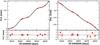 |
Fig. 1 Astrometric motion of GJ 1214 as a function of time. Top panels represent the motion in RA (left) and Dec (right). Bottom panels show the residuals to the astrometric fit. The rms of the residuals is below 1 mas. |
To do this properly, a first realistic estimate of the epoch-to-epoch accuracy is needed. The outputs of the astrometric processing are the astrometric parameters of the target star and of all the other objects in the field. By combining the residuals of all the reference stars from all the epochs, we can compute the expected uncertainty per epoch. Doing this, we obtain an epoch-to-epoch accuracy of ~1.3 mas on both RA and Dec. Since the reference stars are fainter than the target, this is a conservative estimate of the real precision for the target. The star itself, which is not included in the reference frame, shows a standard deviation in the residuals of 1.0 mas/epoch, which is also consistent with the expected CAPSCam performance, assuming 20 min of on-sky observations per epoch (see Boss et al. 2009). Then, we simulate 105 synthetic sets of astrometric observations (same format as Table 1) using the nominal parallax and proper motion at the same epochs of observation. Random Gaussian noise with a single epoch uncertainty of 1.3 mas is injected into each synthetic data set and the 5 astrometric parameters are derived. The standard deviation of each parameter over the 105 solutions is the corresponding uncertainty. The obtained uncertainty for the differential parallax is 0.44 mas and corresponds to a relative precision of ~0.6%. We note that this Monte Carlo method implicitly accounts for parameter correlation (see discussion in Faherty et al. 2012). The differential astrometric measurements used to measure the differential parallax and proper motion of GJ 1214 are given in Table 1. The best fit solution over-plotted with the astrometric epochs is shown in Fig. 1.
The measured parallax is relative to the reference stars. Since they are not at infinite distances, these reference stars also have parallactic motion. As a result, the average parallax of the reference frame cannot be derived from the astrometric observations alone. We obtain this average parallax (also called the parallax zero-point correction) using catalog photometry for the reference stars using the procedure described in Anglada-Escudé et al. (2012b) with 19 reference stars with good CAPSCam astrometry (root mean square (rms) of the residuals below 2.0 mas/epoch) and reliable catalog photometry (B < 18 NOMAD and JHKs 2MASS photometry; Zacharias et al. 2005; Skrutskie et al. 2006). For this set of observations, we determine a zero-point correction of − 0.40 ± 0.3 mas. This value, when added to the relative parallax, produces the final absolute parallax measurement in Table 2. The inverse of the parallax in arcseconds is the distance in parsecs (pc) and amounts to 14.55 ± 0.13 pc. The updated BVRIJHKs, W1,W2,W3 and W4 absolute magnitudes for GJ 1214 are presented and discussed in Sect. 3.
Basic astrometric information and results from the analysis of the astrometry.
We note that the measured proper motions are also differential and contain an unknown offset due to the unknown average motion of the background stars (e.g., all galactic plane stars move roughly in the same direction). Even though catalog values are less precise than the ones we obtain, catalog proper motions are usually corrected for proper motion zero-point ambiguities. Differential measurements as well as the suggested values for the proper motion of GJ 1214 (LSPM-NORTH catalog, Lépine & Shara 2005) are also provided in Table 2.
2.2. Radial velocity measurements
The ESO public archive1 contains 21 reduced HARPS spectra of GJ 1214 obtained by Charbonneau et al. (2009). We reanalyzed these public HARPS spectra using our software called HARPS-TERRA (HARPS Template Enhanced Radial velocity Re-analysis Application, Anglada-Escudé & Butler 2012). HARPS-TERRA derives differential radial velocity (RV) measurement by constructing a high signal-to-noise ratio template from the observations and matching it to each spectrum using a least-squares approach. GJ 1214 is faint at optical wavelengths (V ~ 14). As a consequence, very long exposures (2400 s) were required to obtain any signal at all. Still, the typical S/N at 6100 Å is only ~10 so careful construction of the template is a key element in order to achieve the maximum precision. The standard setup of HARPS-TERRA for M dwarfs uses all the echelle apertures redder than the 22nd one (4400 Å < λ < 6800 Å) and adjusts a cubic polynomial to correct for the variability of the blaze function across each echelle order. Detailed algorithms and performance of HARPS-TERRA on a representative sample of stars is given in Anglada-Escudé & Butler (2012). It is worth noticing that error bars listed in 3 are smaller than those in Charbonneau et al. (2009), suggesting a more optimal usage of the Doppler information in the spectra. However, reduced error bars do not guarantee a more accurate orbital fit when the RV variability is dominated by systematic noise (either instrumental or stellar). To account for this, we included an unknown noise term in our Monte Carlo Markov chain runs which had a substantial effect on the derived distributions, especially on the orbital eccentricity (see discussion in Sect. 2.3).
2.3. Orbital solution
As discussed in Carter et al. (2011), uncertainties in the orbital parameters (especially the eccentricity) are the main limitation in the derivation of precise star-planet parameters. Therefore, we are interested not only in the favoured orbital solution, but also in obtaining a realistic numerical representation of the posterior density function of the parameters to propagate them into the estimates of the star-planet properties. These samples are generated using a Bayesian Monte Carlo Markov chain (MCMC) method. We use custom-made MCMC software to combine RV with transit observations and to obtain such distributions. The software is based on the MCMC tools used in Anglada-Escudé et al. (2012b) adapted to the Doppler plus transit problem, and uses a Gibbs sampler. Jump scales of the Gibbs sampler are initialized using the diagonal elements of the covariance matrix at the maximum likelihood solution, and they are adjusted in the first 105 steps (the “burn-in” period) to accept between 10% and 30% of the jump proposals for each parameter. As discussed below, we assume flat priors for all the sampling parameters. As a consequence, the probability of accepting a new state is just the ratio of likelihoods at the current and proposed jump position. An outline of the general MCMC method applied to the Keplerian problem can be found in Ford (2006).
The Keplerian model for the radial velocities is the same as in Anglada-Escudé & Tuomi (2012) and the transit observations are predicted using the recipes given in the NASA Exoplanet Archive webpage2. Transit observations strongly constrain the orbital period, but also put strong restrictions on the sum of the initial mean anomaly M0, the argument of the node ω (also called, mean longitude λ0 = M0 + ω), and the product ecosω (eccentricity and argument of the node). Accordingly, we use λ0 as a free parameter. Since the transit instants explicitly depend on ecosω, esinω and ecosω are sometimes used as the MCMC sampling parameters. We also tested this approach, and, while it has some desirable properties (e.g., symmetry around zero eccentricity) – this parameterization imposes an implicit prior3 that severely biases the estimates of e to artificially larger values (e.g., see Ford 2006; Barros et al. 2011, for similar discussions). Therefore, at the sampling level, we choose those free parameters that, from our point of view, should have flat prior distributions. These are: orbital frequency 1/P, RV semi-amplitude K, mean longitude λ0, argument of the node ω, and eccentricity e. Despite ω being poorly defined and uncertain at low eccentricities, the convergence of the MCMC was substantially improved thanks to the use of λ0 instead of M0, so we find this parametrization convenient and sufficient for our purposes. All the approximate parameter values are already known from previous studies and, therefore, we initialize the MCMCs within 3 standard deviations of the orbital solution proposed by Charbonneau et al. (2009).
HARPS-TERRA radial velocity measurements.
Expected values of the most useful parameter combinations obtained using RV and transit observations.
Real uncertainties in radial velocity measurements are difficult to estimate properly, especially when the star is active. To account for that, we model the uncertainty of the i-th measurement as  , where ϵi are the formal uncertainties derived from HARPS-TERRA (third column in Table 3), and s is a jitter parameter that accounts for the extra systematic noise. In this context, the jitter parameter s is treated as any other free parameter.
We assign a constant uncertainty to each transit instant of 400 s. This uncertainty is 10 times larger than the typical reported formal errors but it is more consistent with the different instants of transit measurements obtained simultaneously by different groups (see Table 8). While the MCMC convergence properties are greatly improved, 400 s is a small fraction of the time-baseline covered by the transits and, as a consequence, the period is still strongly constrained. The transit time measurements have been extracted from Sada et al. (2010), Carter et al. (2011), and Kundurthy et al. (2011).
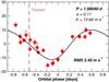 |
Fig. 2 HARPS-TERRA radial velocity measurements folded to the orbital period. The instant of transit is depicted as a dashed vertical line. |
In Table 4, we provide the expected values for the most relevant combination of parameters for physical and transit prediction computations as derived from the combination of 10 MCMC runs with 107 steps each. Figure 2 is an illustration of the maximum a posteriori probability (MAP) solution and is given only for illustration purposes. Since the amplitude of the signal is small compared to the noise, the eccentricity is still poorly constrained. The posterior distribution of the eccentricity has a maximum very close to 0 and monotonically decreases with e (see Fig. 3) implying that close to circular orbits are favored. Because of their significance for the transit observables (e.g., see Sect. 4), an illustration of the MCMC samples of the derived parameters ecosω and esinω is also provided in Fig. 3. Previous estimates of the eccentricity of GJ 1214b (e.g., Charbonneau et al. 2009; Carter et al. 2011) seemed to favor eccentricities close to 0.1, but still compatible with 0. In initial tests, we recovered this same slightly higher eccentricity value if the noise parameter s was fixed to 0. This indicates that previous estimates of the orbital elements were biased due to a non-consistent treatment of the RV uncertainties. Even though stellar jitter dominates the error budget (s ~ 2.9 m s-1), the rms of the MAP solution using the new HARPS-TERRA measurements is lower (3.4 m s-1) than the one reported by Charbonneau et al. (2009, 4.4 m s-1. Given the strong effect of the jitter parameter s on the result, and until more RV measurements become public, we strongly recommend the use of the updated solution in Table 4 for any future work (e.g., in searching for secondary transits). Applying the same 95% confidence level used by Charbonneau et al. (2009), we obtain an upper limit to the eccentricity of 0.23.
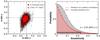 |
Fig. 3 Left: distribution of MCMC states for the derived quantities ecosω and esinω as obtained from 1 MC chain of 107 steps (red) and the combination of 10 chains of 107 steps each (black). Only 1% of the steps are included in this plot to improve visualization. Right: marginalized probability distribution of the eccentricity is shown in black (arbitrary normalization). The corresponding cumulative distribution (red histogram) shows that eccentricities higher than 0.23 are ruled out at a 95% confidence level. |
Another interesting parameter is the minimum mass of GJ 1214b. Even though the new RV amplitude K is smaller (~10.9 m s-1) than the previously reported one (~12.5 m s-1), the updated minimum mass does not change significantly compared to Charbonneau et al. (2009) due to the similar relative increase in the updated stellar mass derived from the new distance determination (see Sect. 4). The origin of the slightly smaller amplitude is likely caused by stellar activity. By analyzing Doppler measurements on known active M dwarfs (e.g., AD Leo, Reiners et al. 2013), we found that the classic HARPS-CCF approach always produces a larger Doppler amplitude than the one derived using HARPS-TERRA (between 1.1 to 1.5 times larger) if a candidate signal is caused by activity. The likely explanation for this is the different sensitivities of the two methods to the changes in the stellar line-profiles. While one could use this effect to obtain a further diagnostic to check the reality of low-mass candidate planets (under investigation), in this case it means that the most likely source of systematic noise comes from the star rather than from the instrument. Doppler follow-up of the star is needed to better understand the origin of the extra noise and to further constrain the orbital solution.
3. Updated properties for GJ 1214
Updated absolute photometry for GJ 1214.
3.1. Metallicity
Two independent techniques, the photometric method by Schlaufman & Laughlin (2010) and the K-band spectroscopic [Fe/H] index by Rojas-Ayala et al. (2012), agree on the metal-richness of GJ 1214, with [Fe/H] = +0.28 dex and [Fe/H] = +0.20 dex, respectively. However, since the [Fe/H] photometric calibrations depend on the distance of the star (to obtain MKs), the photometric value of GJ 1214 needs to be re-calculated using its updated distance. The updated absolute magnitudes are given in Table 5. The updated photometric [Fe/H] values are [Fe/H] = +0.13 dex and [Fe/H] = +0.05 dex, using the Schlaufman & Laughlin (2010) calibration and the recent calibration by Neves et al. (2012), respectively. Considering the dispersions associated with the calibrations (σ0.1–0.15 dex), the estimates are consistent with each other, corroborating that GJ 1214 is a solar or super-solar [Fe/H] star.
A comparative approach can also be performed to confirm the metal-richness of GJ 1214. Figure 4 shows the K-band spectra of Gl 699 (Barnard’s star), Gl 231.1B, and GJ12144. Gl 699 is the second nearest M star to the solar system and its kinematics, Hα activity, and [Fe/H] measurements are consistent with Gl 699 being an old disk/halo star (Gizis 1997; Rojas-Ayala et al. 2012). Gl 231.1B is the low-mass companion of a nearly solar metallicity G0V star ([Fe/H] = –0.04 dex, Valenti & Fischer 2005). The overall shapes of the K-band spectra of all three stars are quite similar (same spectral type), and the morphology of the surface-gravity-sensitive CO bands corresponds to M dwarf stars (log g ~ 5). However, all the absorption features of GJ 1214 are stronger than the ones exhibited by metal-poor Gl 699 ([Fe/H] = –0.39 dex, Rojas-Ayala et al. 2012) and solar metallicity Gl 231.1B. Therefore, also in a relative sense, the strong absorption features favor a high metal content for GJ 1214.
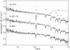 |
Fig. 4 K-band spectra of GJ 1214 (top), Gl 231.1B (middle), and Gl 699 (bottom). All the stars have the same K-band spectral type (same overall shape of their spectra), but different metallicities, as indicated by the strengths of their absorption features. GJ 1214’s metallicity should be at least equal to or higher than solar. |
3.2. Stellar temperature, luminosity, and radius from models
We first provide an overview of previous methods and determinations of the temperature, luminosity, and radius of GJ 1214. In the discovery paper of GJ1214b, (Charbonneau et al. 2009) estimated a Teff = 3026 K and a R⋆ = 0.211 R⊙ for GJ 1214. Kundurthy et al. (2011) obtained Teff = 2949 K and R⋆ = 0.211 R⊙. Constraining parameters to stellar evolution isochrones by Baraffe et al. (1998), Carter et al. (2011) led to estimates of Teff = 3170 K and R⋆ = 0.179 R⊙, assuming that GJ 1214 is an “old star”. However, all these results were based on the distance determination of ~13 pc by van Altena et al. (2001), and reveal that the effective temperature of GJ 1214 is quite uncertain, given all the degeneracies in the evolutionary model used and a low precision distance estimate.
We attempted to get an estimate of the stellar radius using up-to-date interferometric empirical calibrations. For example, Kervella et al. (2004) provides an empirical luminosity-radius calibration that extends to low mass stars and uses absolute magnitudes as the only inputs. We tried different combinations of photometric bands obtaining inconsistent results. All the relations involving optical bands (BVRI) gave values larger than 0.4 R⊙, which are very unrealistic considering the spectral type of GJ 1214. The relations restricted to infrared colors (J,H, and K) provided estimates a bit more realistic (between 0.15 to 0.2 R⊙) but still not fully compatible with each other. We also tried the calibration provided by Demory et al. (2009) that used K band photometry to minimize the metallicity effect on optical magnitudes. In Demory et al. (2009), new measurements of 6 new M dwarfs were presented and a new radius-luminosity calibration was derived. They found a remarkable agreement with the evolutionary models of Baraffe et al. (1998) if the measured radii was plotted against the K absolute magnitude. Using this approach, we obtain a stellar radius of 0.193 R⊙ which, at least, seems to be in the expected range.
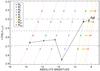 |
Fig. 5 Luminosity as function of absolute magnitude for all the wavebands listed in Table 5. Open diamonds represent the photometry of GJ 1214. The color asterisks represent the BT-Settl-2010 values, and the color dotted lines the linear interpolations between them. The dashed line indicates the mean bolometric luminosity estimated using all the photometry (log (L/L⊙) = −2.57). The dotted-dashed line indicates the mean luminosity with only the BVRI photometry (log (L/L⊙) = −2.73), and the 3 dotted-dashed line the adopted mean luminosity for GJ 1214, derived using only the JHKsW1W1 absolute magnitudes (log (L/L⊙) = −2.44). The lowest bolometric luminosity corresponds to the I magnitude, where the SED is very steep. |
Given that the state-of-the-art empirical relations are not entirely self consistent, we also obtained a new estimate of the effective temperature, luminosity, and radius of GJ 1214 using updated BVRIJHKsW1W2 absolute photometry (Table 5) together with the model atmosphere grid BT-Settl-2010 (Allard et al. 2011)5. The lack of indicators of youth in GJ 1214, such as Hα emission, along with its space motion, gives an age estimate of 3–10 Gyr for the star (Reid & Gizis 2005). This age estimate is also supported by its long rotation period (Charbonneau et al. 2009). Therefore, we fixed the surface gravity of the synthetic spectral models to log g = 5.0 and [M/H] = 0.0. Figure 5 shows the bolometric luminosity as function of absolute magnitude for the BT-Settl-2010 grid. The inferred bolometric luminosities with the JHKsW1W2 photometry are consistent with each other, and higher than the luminosities obtained with the BVRI photometry. Previous synthetic models (e.g. NextGen; Hauschildt et al. 1999) showed a lack of flux in the K band when compared with observed spectra of low-mass stars. New solar abundances and the inclusion of dust grain formation seems to have solved most of the previous discrepancy, allowing the BT-Settl-2010 models to reproduced fairly well the infrared spectral energy distribution (SED) of M-dwarfs (Allard et al. 2011, however, the FeH opacity data is still incomplete for this region). Although models have also been improved at shorter wavelengths (BVRI), they remain too bright in the ultraviolet and visible part of the M dwarf spectra, possibly due to missing sources of opacity in the modeling process (Allard et al. 2011). The effective temperatures and radii corresponding to the best SEDs fit to the 9 wavebands BVRIJHKsW1W2, only BVRI, and only JHKsW1W2, obtained from their respective bolometric luminosities in Fig. 5, are shown in Fig. 6. Given that 1) bolometric luminosities obtained with JHKsW1W2 photometry are consistent with each other; 2) the models provide a better fit at longer wavelengths; and 3) the empirical luminosity-radius provides more self-consistency using NIR colors, the fit with only JHKsW1W2 provides the most reliable results and is the one to be used in deriving further properties of the star-planet system.
The SED fitting using only these NIR bands is further supported by other results. For example in Sect. 4, we will obtain an independent stellar radius estimate (0.211 ± 0.011 R⊙) combining the stellar mass with direct observables from the light curve and Doppler data. Such an estimate is compatible with the value we discussed in this section (~0.2 R⊙). Also, the estimate of the effective temperature (Teff ~ 3250 K) is in excellent agreement with the effective temperature derived from water absorption in K-band by Rojas-Ayala et al. (2012, Teff = 3245. Furthermore, next section shows this Teff also agrees with the one derived from SED fits to the evolutionary models (Baraffe et al. 1998).
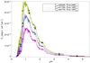 |
Fig. 6 Spectral energy distribution fits for GJ 1214 for the effective temperatures and radii derived from photometry. The magenta, green, and blue SEDs are the spectral templates that represent the values obtained with only BVRI photometry, only JHKsW1W2 photometry, and the 9 wavebands, respectively. All spectral templates have solar metallicity, log g = 5.0 and distance equal to 14.47 pc. The photometry data of GJ 1214 are plotted as black dots. Color dots indicate flux levels of each spectral template integrated over the corresponding filter bandwidth, depicted by the horizontal black lines. The spectral template with Teff = 3250 K and R = 0.2 R⊙ provides the best fit to the infrared photometry of GJ 1214. |
3.3. Stellar mass
Although most of the previously reported mass-radius estimates of GJ 1214 agree, we note that they all assume the trigonometric distance estimate from van Altena et al. (2001). This distance determination has an uncertainty of 10% which is not always accounted for in the aforementioned predictions. We also note that the M1V-M4V spectral type range spans a broad range of stellar masses (from 0.4 to 0.15 M⊙) and effective temperatures (3500 to 2800 K). This makes any mass estimate very sensitive to uncertainties in the parallax mesurement. Given the updated distance, we can apply the Delfosse et al. (2000, hereafter DF00) relations to derive a new mass for GJ 1214 using the absolute J, H and K magnitudes. The masses derived from each photometric band are M(J) = 0.174 M⊙, M(H) = 0.177 M⊙ and M(K) = 0.177⊙, which are in very good agreement.
Another way to obtain an estimate of the mass for GJ 1214 is to compare the absolute magnitude with the synthetic colors from the evolutionary models in Baraffe et al. (1998). Unfortunately, Baraffe et al. (1998) does not contain models for stars with [Fe/H] > 0.0. As a result the optical colors (e.g., B,V,R,I), cannot be properly adjusted to a model. The fit including the BVRIJHK magnitudes has Teff = 2987 K (M = 0.12 M⊙ and is of very low quality (χ2 = 45 for 6 degrees of freedom). The fit to BVR alone give Teff = 2880 K, M = 0.11 M⊙ and a χ2 = 10.0 for 3 degrees of freedom. In contrast, the best fit model obtained from adjusting J, H, and K has a χ2 of 1.92 for 3 degrees of freedom, an effective temperature of 3225 K and a mass of M = 0.172 M⊙. Note that the mass value is very good agreement with the mass estimate derived from the DF00, and the effective temperature is surprisingly close to one from the atmospheric transfer models in the previous Sect. 3.2. How the uncertainty in the stellar mass affects the planet parameters will be discussed and accounted for in Sect. 4.
4. Star-planet parameters from direct observables
4.1. Using the stellar mass as the input
Information from the transit light curves together with the orbital solution can be combined with the stellar mass (or the stellar radius) to fully characterize the bulk properties of the star-planet system. These methods have been developed over the years by different authors and we suggest reading Seager & Mallén-Ornelas (2003), Southworth (2008) and Carter et al. (2011) for more information on the derivations. This subsection describes the relevant relations and the general approach used to derive the star-planet parameters using the stellar mass as the input (mass-input approach).
Assuming a circular orbit for the planet, the transit light curve alone allows one to obtain a direct measurement of the mean stellar density ρ∗ ,circ. Given a fully Keplerian solution from the Doppler data, the stellar density also depends on the eccentricity of the orbit and can be written as 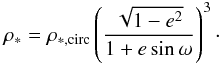 (1)Because no prior information is required from the orbital fit, ρ∗ ,circ is a quantity typically provided by the studies analyzing transit light curves of GJ 1214 (e.g., Carter et al. 2011; Kundurthy et al. 2011). These two studies present the analysis of new light curves and combine them with previous light curves from Charbonneau et al. (2009) and Sada et al. (2010). A weighted mean of ρ∗ ,circ from these two studies will be used in all that follows. The detailed derivation of Eq. (1) was first given by Seager & Mallén-Ornelas (2003) for circular orbits, while Carter et al. (2011) included the dependence on the eccentricity.
With the mean stellar density from Eq. (1) and the stellar mass from the empirical calibrations discussed in Sect. 3.3, one can trivially derive the radius of the star. Using this radius and the transit depth Rp/R∗ (again, a direct observable from the light curves) one then obtains the radius of the planet. The combination of the minimum mass (from RV) and the inclination (from transit light curve) provides the planet’s true mass, which is then combined with the planet radius to finally derive the mean planet density.
Input parameters used to compute the Monte Carlo distributions of the star-planet parameters.
To obtain realistic a posteriori distributions, one needs to assume realistic distributions for the input parameters of the model. The complete list of input parameters used at this point are given in Table 6. For all the values borrowed from the literature, a Gaussian distribution N[μ,σ] is assumed where μ is the preferred value and σ is its published uncertainty. For the parameters derived from the orbital solution in Sect. 2.3, we directly draw samples from the MCMC distributions generated during the orbital analysis. The uncertainty in the stellar mass has to be accounted for at this point. Given the precision in the distance and in the J,H and K photometry, the major source of uncertainty in the mass is due to the actual accuracy of the DF00 calibration. This accuracy is not very well known, but other studies suggest that it should be correct at the 5% level, which is the relative uncertainty we will use for the stellar mass.
The process of solving for all the star-planet parameters is done for the 106 synthetic input sets. The result is a numerical representation of the empirical probability distributions for the derived star-planet properties. In Fig. 7 we show the obtained distributions concerning the planet properties only (mass, radius, density and surface gravity). The surface gravity of the planet can also be derived from observables only using the prescriptions given by (Southworth 2008; combination of light curve parameters and parameters from the orbital solution). Table 7, provides the expected values and standard deviations of the distributions for each derived star-planet parameter.
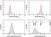 |
Fig. 7 Final probability distributions for most significant bulk properties of GJ 1214b. The mean densities of a few representative Solar system objects are marked as black vertical bars for reference. |
We find that the mean density of GJ 1214b has to be smaller than 2.40 g cm-3 with a 95% confidence level (c.l.), with 1.69 g cm-3 being the expected value of the distribution. An Earth-like density (e.g., ρ > 5.5 g cm3) is thus ruled out at a >99.9% c.l. As illustrated in Fig. 7 this density range confirms that the planet is more similar to a small version of Neptune, or a water dominated body (Berta et al. 2012, e.g., ocean planets,), rather than a scaled-up version of the Earth with a solid surface. This information by itself does not solve the question about the atmospheric composition discussed in the Introduction, but, at least, eliminates the uncertainty in the distance of the star in modeling of the possible planetary structure.
We want to stress that, thanks to the new distance estimate, we now find a remarkably good agreement of the derived stellar radius compared to the one obtained from the SED fit in Sect. 3.2.
As a final test, we reproduced the star-planet parameters using the stellar radius instead of the stellar mass. This consists of doing the following: the stellar radius (SED fit) combined with the mean stellar density (light curve plus RV) gives the stellar mass. Then the stellar mass combined with the RV observables and the inclination (light curve) provides the planet mass. In parallel, the stellar radius with the transit depth (light curve) gives the planet radius, which combined with the mass finally provides the planet density. This approach, however, has a non-obvious drawback. The mass obtained through the stellar density formula depends as the third power on the stellar radius (M∗ ∝ R3), making the stellar mass determination very sensitive to small radius changes. Going the other way around (starting from the mass, derive the radius), the stellar radius depends as M− 1/3, resulting in a much weaker dependence. For example, a 5% uncertainty in the mass translates to a 1.6% uncertainty in the radius. On the other hand, a 5% uncertainty in the radius translates to a 15% uncertainty in the mass. When the uncertainty in the stellar density is also included, this difference is even more pronounced. Therefore, we consider the mass input method a much more robust way of providing a consistent picture. The updated values using the mass input approach for the star-planet parameters are in Table 7 and the marginalized distributions for the relevant planet parameters are depicted in Fig. 7
Suggested new star-planet parameters as derived using the stellar mass as the only input parameter.
Transit time observations used in the orbital fitting.
5. Conclusions
The metallicity of GJ 1214 (and of M dwarfs in general) and its effects on the observable fluxes (e.g., optical fluxes) still require a better understanding, both observationally and theoretically. Even though spectroscopic methods in the NIR are getting better at determining the metal content of cool stars, precise direct measurements of their distances are still required for the characterization of exoplanets around M dwarfs. At least for the stellar masses, the model predictions from the NIR fluxes seem to be in good general agreement with current empirical relations derived from measured masses of M dwarfs in binaries (e.g., DF00). This is fortunate because the stellar mass is the only input parameter required to derive the star-planet bulk properties from direct observables. The fit of the stellar spectral energy distributions to the BT-Settl-2010 model grid also provides consistent estimates in the stellar properties if infrared photometry is used. Even with the remaining ambiguities in the stellar parameters, both approaches (using a stellar mass from empirical relations, or deriving a radius from the absolute fluxes) lead to consistent results for the star-planet bulk properties, but the mass input approach is preferred due to the lower sensitivity of the method to uncertainties in the input parameters. Several studies have been published in recent years trying to better characterize the GJ 1214 star-planet system. The major source of the reported uncertainties came from directly observable quantities that we have improved, collected, and combined here: trigonometric parallax and corresponding absolute fluxes, improved RV measurements, inclusion of all of the transit observations in the derivation of the orbital solution, additional infrared flux measurements, and light curve observables derived from photometric follow-up programs.
We now find remarkable agreement of the derived star properties obtained by comparing the JHK fluxes to up-to-date atmospheric and evolutionary models. All previous studies had to invoke some mechanism (e.g., spot coverage) to justify the mismatch between the predicted versus observed properties of the star. This alone highlights the importance of obtaining direct and accurate distance measurements of low mass stars.
At this time, the quantity that most requires further improvement and/or independent determination is the radius of the star. To our knowledge, this can be observationally achieved with 3 different methods: 1) additional RV measurements to further constrain the orbital eccentricity; 2) direct measurement of the stellar diameter using optical/NIR interferometry (e.g., von Braun et al. 2012); or 3) detection of the secondary transit (whose instant strongly depends on e and ω). We note that GJ 1214 is faint at optical wavelengths compared to other stars observed by high precision RV instruments (e.g., HARPS or HIRES Bonfils et al. 2013; Vogt et al. 2010). In the case of HARPS, integrations of 45 min were required to obtain a precision of ~3.4 m s-1, so a refinement of the orbital eccentricity through additional RV measurements is time-consuming but quite possible. On-going space-based photometric observations in the mid-infrared (e.g., using Warm Spitzer/NASA) should be
able to detect the secondary transit soon and pin down the orbital eccentricity to greater precision. We hope that the updated orbital solution provided here facilitates the task of finding such a secondary transit.
The implicit prior comes from the fact that x = esinω and y = ecosω are cartesian coordinates derived from the polar radial coordinate e and the angle ω. Because MCMCs are based on the integration of a probability distribution, to preserve the flat prior choices for e and ω, one would need to include the Jacobian of the transformation (1/e) as a prior when using x and y as the Markov chain sampling parameters. The use of such a prior is undesirable due to numerical stability issues (divergence for e = 0).
These spectra are part of the K-band spectral atlas by Rojas-Ayala et al. (2012), and available to the community in the online version of that article.
Acknowledgments
We thank the referee D. Ségransan for useful comments that helped improving the manuscript. G.A. has been partially supported by a Carnegie Postdoctoral Fellowship and by NASA Astrobiology Institute grant NNA09DA81A. B.R. thanks the staff and telescope operators of Palomar Observatory for their support. The CAPS team (APB, AJW, GA) thanks the staff and telescope operators of Las Campanas Observatory for the very succesful observing runs and the Carnegie Observatories for continuous support of the CAPS project. We thank France Allard for helpful discussions about various topics. Part of this work is based on data obtained from the ESO Science Archive Facility. This research has made use of NASA’s Astrophysics Data System Bibliographic Services, the SIMBAD database, operated at CDS, Strasbourg, France. This publication makes use of data products from the Two Micron All Sky Survey, which is a joint project of the University of Massachusetts and the Infrared Processing and Analysis Center/California Institute of Technology, funded by the National Aeronautics and Space Administration and the National Science Foundation. This publication makes use of data products from the Wide-field Infrared Survey Explorer, which is a joint project of the University of California, Los Angeles, and the Jet Propulsion Laboratory/California Institute of Technology, funded by the National Aeronautics and Space Administration.
References
- Allard, F., Homeier, D., & Freytag, B. 2011 [arXiv:1112.3591] [Google Scholar]
- Anglada-Escudé, G., & Butler, R. P. 2012, ApJS, 200, A15 [CrossRef] [Google Scholar]
- Anglada-Escudé, G., & Tuomi, M. 2012, A&A, 548, A58 [NASA ADS] [CrossRef] [EDP Sciences] [Google Scholar]
- Anglada-Escudé, G., Arriagada, P., Vogt, S. S., et al. 2012a, ApJ, 751, L16 [NASA ADS] [CrossRef] [Google Scholar]
- Anglada-Escudé, G., Boss, A. P., Weinberger, A. J., et al. 2012b, ApJ, 746, 37 [NASA ADS] [CrossRef] [Google Scholar]
- Baraffe, I., Chabrier, G., Allard, F., & Hauschildt, P. H. 1998, A&A, 337, 403 [NASA ADS] [Google Scholar]
- Barros, S. C. C., Faedi, F., Collier Cameron, A., et al. 2011, A&A, 525, A54 [NASA ADS] [CrossRef] [EDP Sciences] [Google Scholar]
- Bean, J. L., Miller-Ricci Kempton, E., & Homeier, D. 2010, Nature, 468, 669 [NASA ADS] [CrossRef] [PubMed] [Google Scholar]
- Bean, J. L., Désert, J.-M., Kabath, P., et al. 2011, ApJ, 743, 92 [NASA ADS] [CrossRef] [Google Scholar]
- Berta, Z. K., Charbonneau, D., Désert, J.-M., et al. 2012, ApJ, 747, 35 [NASA ADS] [CrossRef] [Google Scholar]
- Bonfils, X., Delfosse, X., Udry, S., et al. 2013, A&A, 549, A109 [NASA ADS] [CrossRef] [EDP Sciences] [Google Scholar]
- Boss, A. P., Weinberger, A. J., Anglada-Escudé, G., et al. 2009, PASP, 121, 1218 [NASA ADS] [CrossRef] [Google Scholar]
- Carter, J. A., Winn, J. N., Holman, M. J., et al. 2011, ApJ, 730, 82 [NASA ADS] [CrossRef] [Google Scholar]
- Charbonneau, D., Berta, Z. K., Irwin, J., et al. 2009, Nature, 462, 891 [NASA ADS] [CrossRef] [PubMed] [Google Scholar]
- Croll, B., Albert, L., Jayawardhana, R., et al. 2011, ApJ, 736, 78 [NASA ADS] [CrossRef] [Google Scholar]
- Cutri, R. M., Wright, E. L., Conrow, T., et al. 2011, Explanatory Supplement to the WISE Preliminary Data Release Products, Tech. Rep., IPAC/CalTech [Google Scholar]
- Dawson, P. C., & Forbes, D. 1992, AJ, 103, 2063 [NASA ADS] [CrossRef] [Google Scholar]
- Delfosse, X., Forveille, T., Ségransan, D., et al. 2000, A&A, 364, 217 [NASA ADS] [Google Scholar]
- Demory, B.-O., Ségransan, D., Forveille, T., et al. 2009, A&A, 505, 205 [NASA ADS] [CrossRef] [EDP Sciences] [Google Scholar]
- Désert, J.-M., Bean, J., Miller-Ricci Kempton, E., et al. 2011, ApJ, 731, L40 [NASA ADS] [CrossRef] [Google Scholar]
- Faherty, J., Burgasser, A. J., Walter, F. M., et al. 2012, ApJ, 752, 56 [NASA ADS] [CrossRef] [Google Scholar]
- Ford, E. B. 2006, ApJ, 642, 505 [NASA ADS] [CrossRef] [Google Scholar]
- Gizis, J. E. 1997, AJ, 113, 806 [NASA ADS] [CrossRef] [Google Scholar]
- Hauschildt, P. H., Allard, F., Ferguson, J., et al. 1999, ApJ, 525, 871 [NASA ADS] [CrossRef] [Google Scholar]
- Kervella, P., Thévenin, F., Di Folco, E., & Ségransan, D. 2004, A&A, 426, 297 [NASA ADS] [CrossRef] [EDP Sciences] [Google Scholar]
- Kundurthy, P., Agol, E., Becker, A. C., et al. 2011, ApJ, 731, 123 [NASA ADS] [CrossRef] [Google Scholar]
- Lépine, S., & Shara, M. M. 2005, AJ, 129, 1483 [NASA ADS] [CrossRef] [Google Scholar]
- Mayor, M., Bonfils, X., Forveille, T., et al. 2009, A&A, 507, 487 [NASA ADS] [CrossRef] [EDP Sciences] [Google Scholar]
- Neves, V., Bonfils, X., Santos, N. C., et al. 2012, A&A, 538, A25 [NASA ADS] [CrossRef] [EDP Sciences] [Google Scholar]
- Reid, I. N., & Gizis, J. E. 2005, PASP, 117, 676 [NASA ADS] [CrossRef] [Google Scholar]
- Reiners, A., Shulyak, D., Anglada-Escudé, G., et al. 2013, A&A, accepted [Google Scholar]
- Rojas-Ayala, B., Covey, K. R., Muirhead, P. S., & Lloyd, J. P. 2012, ApJ, 748, 93 [NASA ADS] [CrossRef] [Google Scholar]
- Sada, P. V., Deming, D., Jackson, B., et al. 2010, ApJ, 720, L215 [NASA ADS] [CrossRef] [Google Scholar]
- Schlaufman, K. C., & Laughlin, G. 2010, A&A, 519, A105 [NASA ADS] [CrossRef] [EDP Sciences] [Google Scholar]
- Seager, S., & Mallén-Ornelas, G. 2003, ApJ, 585, 1038 [NASA ADS] [CrossRef] [Google Scholar]
- Skrutskie, M. F., Cutri, R. M., Stiening, R., et al. 2006, AJ, 131, 1163 [NASA ADS] [CrossRef] [Google Scholar]
- Southworth, J. 2008, MNRAS, 386, 1644 [NASA ADS] [CrossRef] [Google Scholar]
- Valenti, J. A., & Fischer, D. A. 2005, ApJS, 159, 141 [NASA ADS] [CrossRef] [MathSciNet] [Google Scholar]
- van Altena, W. F., Lee, J. T., & Hoffleit, E. D. 2001, VizieR Online Data Catalog: I/238A [Google Scholar]
- Vogt, S. S., Butler, R. P., Rivera, E. J., et al. 2010, ApJ, 723, 954 [NASA ADS] [CrossRef] [EDP Sciences] [Google Scholar]
- von Braun, K., Boyajian, T. S., Kane, S. R., et al. 2012, ApJ, 753, 171 [NASA ADS] [CrossRef] [Google Scholar]
- Zacharias, N., Monet, D. G., Levine, S. E., et al. 2005, VizieR Online Data Catalog: I/297 [Google Scholar]
All Tables
Expected values of the most useful parameter combinations obtained using RV and transit observations.
Input parameters used to compute the Monte Carlo distributions of the star-planet parameters.
Suggested new star-planet parameters as derived using the stellar mass as the only input parameter.
All Figures
|
Fig. 1 Astrometric motion of GJ 1214 as a function of time. Top panels represent the motion in RA (left) and Dec (right). Bottom panels show the residuals to the astrometric fit. The rms of the residuals is below 1 mas. |
| In the text | |
|
Fig. 2 HARPS-TERRA radial velocity measurements folded to the orbital period. The instant of transit is depicted as a dashed vertical line. |
| In the text | |
|
Fig. 3 Left: distribution of MCMC states for the derived quantities ecosω and esinω as obtained from 1 MC chain of 107 steps (red) and the combination of 10 chains of 107 steps each (black). Only 1% of the steps are included in this plot to improve visualization. Right: marginalized probability distribution of the eccentricity is shown in black (arbitrary normalization). The corresponding cumulative distribution (red histogram) shows that eccentricities higher than 0.23 are ruled out at a 95% confidence level. |
| In the text | |
|
Fig. 4 K-band spectra of GJ 1214 (top), Gl 231.1B (middle), and Gl 699 (bottom). All the stars have the same K-band spectral type (same overall shape of their spectra), but different metallicities, as indicated by the strengths of their absorption features. GJ 1214’s metallicity should be at least equal to or higher than solar. |
| In the text | |
|
Fig. 5 Luminosity as function of absolute magnitude for all the wavebands listed in Table 5. Open diamonds represent the photometry of GJ 1214. The color asterisks represent the BT-Settl-2010 values, and the color dotted lines the linear interpolations between them. The dashed line indicates the mean bolometric luminosity estimated using all the photometry (log (L/L⊙) = −2.57). The dotted-dashed line indicates the mean luminosity with only the BVRI photometry (log (L/L⊙) = −2.73), and the 3 dotted-dashed line the adopted mean luminosity for GJ 1214, derived using only the JHKsW1W1 absolute magnitudes (log (L/L⊙) = −2.44). The lowest bolometric luminosity corresponds to the I magnitude, where the SED is very steep. |
| In the text | |
|
Fig. 6 Spectral energy distribution fits for GJ 1214 for the effective temperatures and radii derived from photometry. The magenta, green, and blue SEDs are the spectral templates that represent the values obtained with only BVRI photometry, only JHKsW1W2 photometry, and the 9 wavebands, respectively. All spectral templates have solar metallicity, log g = 5.0 and distance equal to 14.47 pc. The photometry data of GJ 1214 are plotted as black dots. Color dots indicate flux levels of each spectral template integrated over the corresponding filter bandwidth, depicted by the horizontal black lines. The spectral template with Teff = 3250 K and R = 0.2 R⊙ provides the best fit to the infrared photometry of GJ 1214. |
| In the text | |
|
Fig. 7 Final probability distributions for most significant bulk properties of GJ 1214b. The mean densities of a few representative Solar system objects are marked as black vertical bars for reference. |
| In the text | |
Current usage metrics show cumulative count of Article Views (full-text article views including HTML views, PDF and ePub downloads, according to the available data) and Abstracts Views on Vision4Press platform.
Data correspond to usage on the plateform after 2015. The current usage metrics is available 48-96 hours after online publication and is updated daily on week days.
Initial download of the metrics may take a while.