| Issue |
A&A
Volume 551, March 2013
|
|
|---|---|---|
| Article Number | A60 | |
| Number of page(s) | 6 | |
| Section | Galactic structure, stellar clusters and populations | |
| DOI | https://doi.org/10.1051/0004-6361/201117229 | |
| Published online | 22 February 2013 | |
CV1 in the globular cluster M 22: confirming its nature through X-ray observations and optical spectroscopy
1 Université de Toulouse, UPS-OMP, IRAP, Toulouse, France
e-mail: This email address is being protected from spambots. You need JavaScript enabled to view it.
2 CNRS, IRAP, 9 avenue du Colonel Roche, BP 44346, 31028 Toulouse Cedex 4, France
3 Laboratoire AIM, CEA/DSM/IRFU/SAp, CNRS, Université Paris 7 Denis Diderot, CEA Saclay, Bat. 709, 91191 Gif-sur-Yvette, France
4 Harvard-Smithsonian Center for Astrophysics, 60 Garden Street, MS-67, Cambridge, MA 02138, USA
Received: 10 May 2011
Accepted: 20 December 2012
Abstract
Context. Observations of cataclysmic variables in globular clusters appear to show a dearth of outbursts compared to those observed in the field. A number of explanations have been proposed, including low mass-transfer rates and/or moderate magnetic fields implying higher mass white dwarfs than the average observed in the field. Alternatively this apparent dearth may be simply a selection bias.
Aims. We examine multi-wavelength data of a new cataclysmic variable, CV1, in the globular cluster M 22 to try to constrain its period and magnetic nature, with an aim at understanding whether globular cluster cataclysmic variables are intrinsically different from those observed in the field.
Methods. We use the sub-arcsecond resolution of the Chandra ACIS-S to identify the X-ray counterpart to CV1 and analyse the X-ray spectrum to determine the spectral model that best describes this source. We also examine the low resolution optical spectrum for emission lines typical of cataclysmic variables. Cross correlating the Hα line in each individual spectrum also allows us to search for orbital motion.
Results. The X-ray spectrum reveals a source best-fitted with a high-temperature bremsstrahlung model and an X-ray unabsorbed luminosity of 1.8 × 1032 erg s-1 (0.3–8.0 keV), which are typical of cataclysmic variables. Optical spectra reveal Balmer emission lines, which are indicative of an accretion disc. Potential radial velocity in the Hα emission line is detected and a period for CV1 is proposed.
Conclusions. These observations support the CV identification. The radial velocity measurements suggest that CV1 may have an orbital period of ~7 h, but further higher resolution optical spectroscopy of CV1 is needed to unequivocally establish the nature of this CV and its orbital period.
Key words: globular clusters: individual: M 22 / binaries: close / stars: dwarf novae / X-rays: binaries
© ESO, 2013
1. Introduction
Globular clusters (GCs) are very dense groups of old stars, where the most massive stars of the cluster have already evolved away from the main sequence and into compact objects (e.g. neutron stars and white dwarfs). In these dense environments, interactions between cluster members are frequent, and binary systems, including those containing compact objects, can form readily (e.g. Hut et al. 1992). Indeed the number of neutron star X-ray binaries in Galactic GCs scales with the cluster encounter rate (Gendre et al. 2003; Pooley et al. 2003), as do the millisecond pulsars (Abdo et al. 2010), which are believed to be the progeny of the neutron star X-ray binaries (Wijnands & van der Klis 1998). Simulations also show that a large number of close binaries (neutron star X-ray binaries and cataclysmic variables, CVs) should exist in GCs (e.g. Di Stefano & Rappaport 1994; Davies 1997; Ivanova et al. 2006).
Close binaries are extremely difficult to locate in the optical domain because of over-crowding. Two methods that can be exploited to detect close binaries are either (i) to observe the cluster in the X-ray domain where only about 100 sources can be expected (e.g. Servillat et al. 2008a,b; Webb et al. 2006); or (ii) to try to detect variability and/or optical outbursts from the systems (e.g. Servillat et al. 2011; Kaluzny et al. 2010; Kaluzny et al. 1996). With these methods, dozens of interacting binaries in Galactic GCs have been discovered.
Thanks to the proximity of the white dwarf and its companion in a CV, material is accreted from the companion star and stored in the accretion disc around the white dwarf, whilst it loses enough angular momentum to fall onto the compact object. Outbursts are believed to occur when too much material builds up in the disc, increasing both the density and the temperature, until the hydrogen ionises and the viscosity increases sufficiently for the material to fall onto the white dwarf (Osaki 1974; Meyer & Meyer-Hofmeister 1981; Bath & Pringle 1981, etc.). Such outbursts are characterised by a steep rise in the flux by several orders of magnitude. Many types of field CVs show such outbursts every few weeks to years. Comparing the small population of CVs identified in GCs to those known in the field has revealed a striking and unexplained difference. Only very few GC CV outbursts have been observed (e.g. Paresce & de Marchi 1994; Shara et al. 1996b, 1987), and it is unclear why this should be.
It was originally suggested that GC CVs may be mainly magnetic (e.g. the five magnetic CVs in Grindlay 1999). Magnetic CVs have accretion discs that are either partially or totally disrupted by the strong white dwarf magnetic fields, known as intermediate polars, and polars respectively. Material is channelled along the field lines onto the white dwarf, although in the case of intermediate polars, a truncated disc can exist, and these systems can undergo a limited number of outbursts (e.g. Norton & Watson 1989). However, more recently it has been proposed that it may not simply be the magnetic field that is responsible for the lack of outbursts. Dobrotka et al. (2006) suggest that it may be due to a combination of low mass-transfer rates (≲1014 − 15 g s-1) and moderately strong white dwarf magnetic moments (≳1030 G cm3) that could stabilise the CV discs through truncation of inner regions (Meyer & Meyer-Hofmeister 1994) and thus prevent most of them from experiencing frequent outbursts. Ivanova et al. (2006) also suggests that the lack of outbursts are due to higher white dwarf masses in GC CVs compared to those in the field. This would imply that GC CVs are intrinsically different from those in the field. This could be due to the difference in the formation mechanisms of GC and field CVs, where a substantial fraction of cluster CVs are likely to be formed through encounters, rather than from their primordial binaries (Ivanova et al. 2006). Alternatively, the observed phenomenon could simply be due to selection biases, where our knowledge of CVs is limited to a small population of the closest CVs that are frequently observed to outburst, as these are the easiest objects to detect. It has recently been proposed that the majority of CVs may be short period, low mass-transferring systems that therefore show infrequent outbursts (e.g. Uemura et al. 2010). If this is the case, GC CVs may be no different from the field CV population (e.g. Servillat et al. 2011).
Sahu et al. (2001) presents an event in the Galactic GC M 22 in which a star was observed to brighten by approximately three magnitudes in the Hubble Space Telescope (HST) band F814W, over about ten days, and to fade again on a similar timescale. Some interspersed F606W images showed a similar brightening. Sahu et al. (2001) argue that an unseen low-mass star in the cluster had lensed a background bulge star. To test whether this was a lensing event, Anderson et al. (2003) used optical photometry to measure the proper motion of the star that had been seen to brighten and determined that it was part of the cluster. From its variability, its Hα emission, and its coincidence with the Einstein/Rosat source X4/B, Anderson et al. (2003) conclude that this source, which they call CV1, was one of a very small number of confirmed or probable dwarf nova eruptions seen in GCs and the first to be found in such a low-concentration cluster. Bond et al. (2005) confirm the variable nature of this source using a four year light curve of the same source in M 22, based on an analysis of accumulated data from the Micro-lensing Observations in Astrophysics (MOA) survey. From the regularity of the three outbursts detected between 1999 and 2004 and their magnitude, Bond et al. (2005) also propose that this source may be a cataclysmic variable. From the X-ray properties and optical variability, Hourihane et al. (2011) propose that CV1 is a U Gem-type cataclysmic variable.
In this paper we present both Chandra and XMM-Newton archived data for this cluster, along with low-resolution optical spectroscopy of CV1 and discuss the nature of this CV in the context of outbursts from GC CVs.
2. X-ray observations
Chandra observations of the Galactic GC M 22 were made on 24 May, 2005 for 16 ks using the ACIS-S3 cameras (ObsIDs: 7919 and 8566). We used CIAO version 3.4 software and the CALDB v3.4.0 set of calibration files (gain maps, quantum efficiency, quantum efficiency uniformity, effective area). We reprocessed the level-1 event files of both observations without including the pixel randomisation that is added during standard processing. This method slightly improves the point-spread function (PSF).We removed cosmic-ray events that could be detected as spurious faint sources using the tool acis_detect_afterglow, and identified bad pixels with the tool acis_run_hotpix. The event lists were then filtered for grades, status, and good time intervals (GTIs), as in the standard processing. We selected events within the energy range 0.3–10.0 keV.
To obtain a list of source candidates, we employed the CIAO wavelet-based wavdetect tool for source detection in the field of view covered by the four ACIS-I chips. The two energy bands used were the 0.3–10.0 keV band, with all the events that allowed us to detect the faintest sources, and 0.5–6.0 keV that had a higher signal-to-noise ratio, so gave more significant detections. We selected scales of 1.0, 1.4, 2.0, 2.8, 4.0, and 5.6 pixels. The scales were chosen to look for narrow PSF sources on-axis and ensure optimal separation, and larger PSF sources at the edge of the detectors, where the PSF is degraded. We selected a threshold probability of 106, designed to give one false source per 106 pixels. This led to the detection of 50 source candidates. We added to this 33 sources previously detected with XMM-Newton (observation ID: 0112220201, Webb et al. 2004) that fall inside the Chandra field of view. We then used ACIS-Extract to determine the sources detected with a significance greater than 99.999% (Broos et al. 2010). We thus detected 39 sources, each with at least five counts. These sources are given in Table 1.
Using the nH value of 2.2 × 1021 cm-2 (Johnston et al. 1994) and a power law slope of 2.1 (the average of the 39 detected sources), the unabsorbed flux limit of the Chandra observation is 3 × 10-15 erg cm-2 s-1 (0.5–8.0 keV). Using the distance measurement of 3.2 kpc (Harris 1996, December 2010 revision) this translates to an unabsorbed luminosity limit for an object in the cluster of 4 × 1030 erg s-1 (0.5–8.0 keV). This is slightly deeper than the XMM-Newton observation presented in Webb et al. (2004), which has an unabsorbed luminosity limit in the Chandra band and using a distance of 3.2 kpc (0.6 kpc greater than the distance given in Webb et al. 2004) of 7 × 1030 erg s-1. As a result, more sources are detected within the Chandra field of view. All but two of the XMM-Newton sources that fall within the Chandra field of view were detected, see Fig. 1. These two sources, which are below the threshold presented in Webb et al. (2004) but present in the more recently analysed data of the 2XMM catalogue (Watson et al. 2009), may be variable sources. We find that Chandra source 3 is coincident with the position of a newly discovered binary radio pulsar, M22A (Lynch et al. 2011), to within the 2σ error radius of the X-ray source. None of the sources correspond to the two new radio sources that are proposed as black hole binaries (Strader et al. 2012), but the X-ray and radio observations are not simultaneous, which may account for their not being detected.
Thanks to the superior angular resolution of Chandra, the 1σ positional error of the Chandra sources is, for the majority of the sources, sub-arcsecond (see Table 1), compared to the 90% confidence mean statistical error of ⟨ 7.6″ ⟩ for the XMM-Newton sources (Webb et al. 2004). This difference is clearly seen in Fig. 1, where both the Chandra and the XMM-Newton sources are presented, along with their error circles. Also included in Fig. 1 are the possible optical counterparts selected following a search for sources detected with the Anglo Australian Telescope (AAT) Wide Field Imager that were bluer than the GC main sequence stars and that fall within the XMM-Newton X-ray error circles (Webb et al. 2004) and CV1. It is evident from this figure that the majority of the possible optical counterparts are unlikely to be the actual counterpart, as they are not within the smaller Chandra error circle. The position of the source CV1 falls at 18h36m24 70, –23°54′35
 1, with a 1σ error circle of ~1″ (Bond et al. 2005), is, however, coincident within the errors with the Chandra source, see Fig. 1.
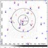 |
Fig. 1 X-ray sources in the direction of M 22. Chandra sources, with the numbers given in Table 1 are shown with their 1σ error circles (red). The larger (blue) error circles show the XMM-Newton sources detected in the field of view, as extracted from the catalogue 2XMM (Watson et al. 2009). The crosses show the positions of the possible optical counterparts. The two largest circles centred on the image are the core radius (1.33′) and the half mass radius (3.36′) (Harris 1996, December 2010 revision). |
To confirm that Chandra source 2 is the X-ray counterpart, we extracted the X-ray spectrum, and fitted this with simple models. Equally good fits are obtained for a power law fit ( cm-2,
cm-2,  ,
,  , 12 d.o.f., errors are 90%) or a bremsstrahlung (
 cm-2,
cm-2,  keV,
keV,  , 12 d.o.f.). These fits are consistent with those found by Hourihane et al. (2011) with the same data sets. Using the latter fit we find an unabsorbed flux of 1.49(
 erg cm-2 s-1 (0.3–8.0 keV, error 1σ), which translates to an unabsorbed luminosity of 1.83 × 1032 erg s-1 (0.3–8.0 keV) at the distance of the cluster. The data and the bremsstrahlung fit can be seen in Fig. 2.
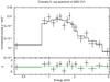 |
Fig. 2 Upper: Chandra spectrum of CV1, fitted with a bremsstrahlung model, as described in Sect. 2. Lower: residuals to the fit. |
3. Optical observations and data reduction
Observations were made with the VIsible Multi-Object Spectrograph (VIMOS) on the 8.2 m Melipal telescope of the European Southern Observatory Very Large Telescope (VLT), with the aim of identifying the X-ray sources given in Webb et al. (2004). For further information about the instrument used here see Le Fèvre et al. (2004). The pre-images were taken on 14 April, 2004 (field 1, centred on 18:35:58.2, –23:57:39.9, J2000) and on 16 May 2004 (field 2, centred on 18:36:34.0, –23:57:39.9, J2000). These images were made using the U filter and were of 120 and 60 s respectively. The positions from the AAT data were transformed onto the VIMOS instrument coordinate system using the VLT supplied VIMOS mask preparation software (VMMPS) and then masks for the spectroscopic observations were defined with the same package. Four fairly bright stars that were well spaced out on each of the four CCDs were allotted slits to be used for alignment purposes. We placed slits of 1′′ width (4.88 pixels) and 14′′ in length (68 pixels) on each of the targets. The remaining slits were placed on random other stars in the field of view.
The spectroscopic observations were carried out in service mode on three different nights, June 9 and 22 and July 9, 2004, and are summarised in Table 2. The blue grism has a range of 3700–6700 Å, and the ESO VIMOS web pages give a spectral resolution (λ/Δ λ) of 180 for a 1′′ slit, with a dispersion of 5.35 Å/pixel. The red grism has a range of 5500–9500 Å, and the ESO VIMOS web pages give a spectral resolution of 210 for a 1′′ slit and a dispersion of 7.14 Å/pixel. The seeing was typically below 0.8′′, except for the last night when it exceeded 1′′. Flat-field lamp and helium-argon arc lamp observations were taken to flat-field and wavelength-calibrate the data. The flux standard stars LTT 1020, NGC 7293, and Feige 110 were also observed during the night to flux calibrate the targets.
Summary of the optical observations presented.
The VIMOS interactive pipeline and graphical interface (VIPGI, Scodeggio et al. 2005). The data were bias-subtracted, but the dark current was negligible (<1 e−/pixel), so no dark correction was carried out. Flat-field corrections were also made and the spectra were wavelength-calibrated using the arc lamps, which gave the wavelength measurements good to approximately 1 Å. Due to the very high density of sources, each spectrum was extracted using an IDL program written specifically to estimate the sky contribution in each slit and then to use an optimal extraction method (Horne 1986) to obtain the spectrum. The flux standards that had been observed throughout the observations, on each CCD individually and in both wavelength regions were extracted in a similar manner. Using these observations, coupled with the spectral energy distributions given in Oke (1990) and Hamuy et al. (1994), we corrected for the instrument response and flux-calibrated the spectra. We also dereddened the spectra using E(B − V) = 0.38 ± 0.02 (Monaco et al. 2004).
In the following we concentrate on the optical spectra of CV1, as this counterpart is the only one that falls within the Chandra error circle, see Sect. 2. These spectra were taken during the field 2 observations, see Table 2.
4. The candidate cataclysmic variable CV1
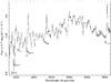 |
Fig. 3 Dereddened blue spectrum of the optical counterpart to source 36. The strongest Balmer lines are seen in emission. Also evident are the Ca H and K lines (rest wavelengths 3968.5 Å and 3933.7 Å respectively). |
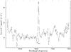 |
Fig. 4 Dereddened red spectrum of the optical counterpart to source 36. The Hα line as well as a possible He I (5876 Å) are seen in emission. Only the spectrum up to 7500 Å is presented as redder than this the telluric absorption and fringing makes the spectrum very noisy. |
We extracted optical spectra of CV1 as described in Sect. 3. We estimated that the brighter neighbour contributes approximately 10% to our source’s spectrum, by plotting the PSF of the two sources relative to each other and measuring the amount of flux from the neighbour within the PSF of CV1. We then subtracted this flux from our target. The neighbouring star’s spectrum contains no emission lines and appears to be a mid K-type star. To check that this procedure introduced no strange features into our spectra, we extracted the CV1 spectra using only the region in the slit where CV1 dominated the emission. We therefore did not need to subtract the close neighbour. This obviously has an impact on the total flux. With this method we extracted spectra with only a third of the flux, but the spectra using the two methods are none the less very similar. The optical spectrum of the target (see Figs. 3 and 4) shows Balmer line emission that are indicative of accretion. We give the equivalent widths of the principal Balmer lines (Å) in Table 3 along with their fluxes. We have identified the Ca II H and K absorption lines at 3968.5 and 3933.7 Å, which we assume are due to the late type companion star (see below). There may also be some evidence for weak Ti0 bands in the red spectrum at 7055 Å, which would indicate that it is an early M-star if they come from the secondary. We also note that the flux in the red spectrum is slightly higher than that presented in the blue spectra. CV1 was declining from an outburst when the red spectra were taken (Hourihane et al. 2011), whereas it was in quiescence when the blue spectra were taken (Hourihane et al. 2011), which may explain the variation in flux.
Equivalent widths of the principal spectral lines in the optical spectrum of CV1.
Seven observations were made of field 2 with the red grism and four for field 1. Four observations were also made of each of the fields observed with the blue grism, see Table 2. Multiple, short observations were made so as not to saturate the brightest counterparts with a single long exposure. We have taken advantage of the fact that the individual optical spectra of CV1 contain enough counts to identify the main emission lines in all spectra. We first subtracted the continuum before cross-correlating the region around the Hα line (6540–6600 Å, as this region is present in both the red and the blue spectra), with the total spectrum (summed red spectra) of a late G/early K-type star believed to be in the cluster, using the IRAF (Tody 1993) task fxcor1. The results are presented in Fig. 5 with the errors bars given using the fxcor. A critical analysis of these errors is given below. We show a fit that assumes a circular orbit with an amplitude of  km s-1 and a period of
  h (
h ( (8 d.o.f.), errors are given at the 90% level). Other periods between ~2.5 and 24 h give acceptable fits i.e.
  –2.0 (8 d.o.f.), indicating that, although the error on the period is small, there are other periods that can give almost as good a fit and therefore may be equally valid. Cross correlating with another star in the cluster means that we can not measure the proper motion of the cluster itself. These observations suggest that we may have detected orbital motion. Although less significant, we see a similar trend from the other Balmer lines visible in the blue spectra, which are likely to be coming from the disc and which appear to be an opposite trend from the calcium H- and K-lines, as expected if these lines originate in the secondary star.
To investigate the reliability of the fxcor errors, we also estimated errors by considering the accuracy with which the central wavelength of the Hα line can be estimated. We fitted a Gaussian to the Hα line and determined the 90% error on the the central wavelength. We then used that to calculate the error on the cross correlation. This error is much larger and varies between 18 and 90 km s-1. Fitting the radial velocity data with these larger error bars with either a constant (i.e. assuming no variability expected), gives a  (10 d.o.f.). Fitting with a constant+sinusoid (i.e. assuming some radial velocity variability) gives
  (8 d.o.f.). This suggests that constant+sinusoid is preferred, but the reduced chi-squared values are very low, due to the inordinately large errors. Fitting the data with the errors given by fxcor we find
  (10 d.o.f.) for a simple constant and
  (8 d.o.f.) for a constant + sinusoid. Again, the sinusoid is preferred. We checked the fxcor cross correlation procedure for our data by cross correlating the summed late G-/early K-star with individual spectra of the same source (in both the blue and the red) and find that the position of the Hα line does not vary to within ±8 km s-1. Cross correlating the same star with CV1 reveals radial velocities between –61 and +17 km s-1 (see Fig. 5). It therefore seems probable that we have detected radial velocity variability in CV1 and that the errors could be considered to be as low as ±8 km s-1, which is similar to the fxcor errors.
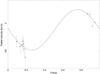 |
Fig. 5 Radial velocities and errors of the Hα line in the optical spectrum of CV1. The solid line shows the best sinusoidal fit to these data. The points shown with filled squares are the radial velocity measurements made with the red spectra. The remaining four data points are the radial velocity measurements made with the blue spectra. |
5. Discussion and conclusion
The Chandra source 2 and CV1 are coincident within the errors. Employing the method used in Zane et al. (2008), we calculated the probability that CV1 is aligned by chance coincidence with Chandra source 2. This probability is given as 1 − e− πμr2, where μ is the measured object density in the Chandra field of view, and r is the radius of the HST error circle. We find a probability of a chance coincidence of 2.34 × 10⁻⁴, confirming CV1 as the optical counterpart to source 2. The X-ray flux and spectrum of source 2 are consistent with that of known CVs (e.g. Baskill et al. 2005; Byckling et al. 2010) and supports the hypothesis that the X-ray source is a CV and therefore the X-ray counterpart to CV1. The dereddened optical spectrum presented here substantiate that CV1 exhibits a blue excess compared to a main sequence star, shows Balmer emission lines endorsing the CV nature. Anderson et al. (2003) note that the object they observed using photometry was redder than the main sequence, however, this may be due in part to the Hα emission, which is present in the V606, R675, and I814 broad band filters they used. We also see that the emission is relatively strong in the red.
From the magnitudes presented in Anderson et al. (2003) and Hourihane et al. (2011) we can determine the expected period as follows. The absolute magnitude of this source using the distance of Harris (1996, December 2010 revision) is around 6.3 (V-band and assuming that the CV is in M 22). Using the correlation between brightness and orbital period (Warner 1987), in the same way as Anderson et al. (2003), but using the revised distance and therefore revised absolute magnitude, implies a period of around 10–11 h. Taking the peak V-magnitude of around three magnitudes brighter than the quiescent value (Anderson et al. 2003) indicates a similar period. However, Patterson (2011) presents a revised version of this correlation, by using precise distances to the 46 CVs studied. He then extrapolates this to study the shortest period CVs. Without correcting CV1 for its inclination, which is at present unknown, the Patterson (2011) relationship reveals a period of around nine hours. The data presented in this paper could also be fitted with a period of around nine hours, however, the  then rises from 1.20 to 1.91 (8 d.o.f.) for the fit with a longer period. However, there is a lot of scatter in the data points presented in Patterson (2011), so a peak outburst magnitude of MV = 3.2 is still compatible with the period of about seven hours. It should also be noted that Anderson et al. (2003) show that CV1 is redder than the main sequence, as mentioned above. They state that this may indicate a secondary that could be larger than a normal main-sequence star, which may raise the question of the validity of these relations for this particular source and indeed we do see that this CV is fairly red. More and higher resolution, higher signal-to-noise observations will be necessary to confirm the true nature of this CV and validate its period.
As outlined in Sect. 1, it has been proposed on numerous occasions that GC CVs may be magnetic in nature, which may help explain the dearth of outbursts observed from these objects. A period of around seven hours may also lend further support for this type of object. Dobrotka et al. (2006) propose that the dearth of outbursts in GC CVs may be due to both low mass-transfer rates and truncated inner discs, as seen in IPs. CV1 appears to show fewer outbursts than many of the well studied CVs, i.e. Shara et al. (1996a), which presents 21 well studied CVs that have an average of ~29 days between outbursts and an average duration of ~15 days. It would then be expected to observe about eight outbursts per year from these CVs on average. Comparing the three outbursts that were observed between 1999 and 2004, if they were indeed the only outbursts during this time, CV1 appears to rarely show outbursts. However, the CVs presented in Shara et al. (1996a) have been well studied because they show regular outbursts. It is likely that the majority of CVs show quite distinct characteristics, with much less regular outbursts (Shara et al. 2005). This would then imply that the lack of observed GC CV outbursts is simply related to selection biases.
Acknowledgments
The authors are extremely grateful to the anonymous referee who raised a number of very valuable points and thus helped to improve the manuscript enormously. M.S. acknowledges supports from NASA/Chandra grants AR9-0013X and GO0-11063X and NSF grant AST-0909073. This research has made use of data obtained from the Chandra Data Archive, and software provided by the Chandra X-ray Center (CXC) in the application package CIAO. It was also based on observations made with ESO Telescopes at the Paranal Observatory under programme ID 073.D-0392(A) and (B), and XMM-Newton, an ESA science mission with instruments and contributions directly funded by ESA Member States and NASA.
References
- Abdo, A. A., Ackermann, M., & Ajello, M. 2010, A&A, 524, A75 [NASA ADS] [CrossRef] [EDP Sciences] [Google Scholar]
- Anderson, J., Cool, A. M., & King, I. R. 2003, ApJ, 597, L137 [NASA ADS] [CrossRef] [Google Scholar]
- Baskill, D. S., Wheatley, P. J., & Osborne, J. P. 2005, MNRAS, 357, 626 [NASA ADS] [CrossRef] [Google Scholar]
- Bath, G. T., & Pringle, J. E. 1981, MNRAS, 194, 967 [NASA ADS] [CrossRef] [Google Scholar]
- Bond, I. A., Abe, F., Eguchi, S., et al. 2005, ApJ, 620, L103 [NASA ADS] [CrossRef] [Google Scholar]
- Broos, P. S., Townsley, L. K., Feigelson, E. D., et al. 2010, ApJ, 714, 1582 [NASA ADS] [CrossRef] [Google Scholar]
- Byckling, K., Mukai, K., Thorstensen, J. R., & Osborne, J. P. 2010, MNRAS, 408, 2298 [NASA ADS] [CrossRef] [Google Scholar]
- Davies, M. B. 1997, MNRAS, 288, 117 [NASA ADS] [CrossRef] [Google Scholar]
- Di Stefano, R., & Rappaport, S. 1994, ApJ, 423, 274 [NASA ADS] [CrossRef] [Google Scholar]
- Dobrotka, A., Lasota, J., & Menou, K. 2006, ApJ, 640, 288 [NASA ADS] [CrossRef] [Google Scholar]
- Gendre, B., Didier, B., & Webb, N. A. 2003, A&A, 403, L11 [NASA ADS] [CrossRef] [EDP Sciences] [Google Scholar]
- Grindlay, J. E. 1999, in Annapolis Workshop on Magnetic Cataclysmic Variables, ASP Conf. Ser. 157, eds. C. Hellier, & K. Mukai, 377 [Google Scholar]
- Hamuy, M., Suntzeff, N. B., Heathcote, S. R., et al. 1994, PASP, 106, 566 [NASA ADS] [CrossRef] [Google Scholar]
- Harris, W. E. 1996, AJ, 67, 1487 [NASA ADS] [CrossRef] [Google Scholar]
- Horne, K. 1986, PASP, 98, 609 [NASA ADS] [CrossRef] [EDP Sciences] [Google Scholar]
- Hourihane, A. P., Callanan, P. J., Cool, A. M., & Reynolds, M. T. 2011, MNRAS, 414, 184 [NASA ADS] [CrossRef] [Google Scholar]
- Hut, P., McMillan, S., Goodman, J., et al. 1992, PASP, 104, 981 [NASA ADS] [CrossRef] [Google Scholar]
- Ivanova, N., Heinke, C. O., Rasio, F. A., et al. 2006, MNRAS, 372, 1043 [NASA ADS] [CrossRef] [Google Scholar]
- Johnston, H. M., Verbunt, F., & Hasinger, G. 1994, A&A, 289, 763 [NASA ADS] [Google Scholar]
- Kaluzny, J., Kubiak, M., Szymanski, M., et al. 1996, A&AS, 120, 139 [NASA ADS] [CrossRef] [EDP Sciences] [Google Scholar]
- Kaluzny, J., Thompson, I. B., Krzeminski, W., & Zloczewski, K. 2010, Acta Astron., 60, 245 [NASA ADS] [Google Scholar]
- LeFèvre, O., Vettolani, G., Paltani, S., et al. 2004, A&A, 428, 1043 [NASA ADS] [CrossRef] [EDP Sciences] [Google Scholar]
- Lynch, R. S., Ransom, S. M., Freire, P. C. C., & Stairs, I. H. 2011, ApJ, 734, 89 [NASA ADS] [CrossRef] [Google Scholar]
- Meyer, F., & Meyer-Hofmeister, E. 1981, A&A, 104, L10 [NASA ADS] [Google Scholar]
- Meyer, F., & Meyer-Hofmeister, E. 1994, A&A, 288, 175 [NASA ADS] [Google Scholar]
- Monaco, L., Pancino, E., Ferraro, F. R., & Bellazzini, M. 2004, MNRAS, 349, 1278 [NASA ADS] [CrossRef] [Google Scholar]
- Norton, A. J., & Watson, M. G. 1989, MNRAS, 237, 853 [NASA ADS] [CrossRef] [Google Scholar]
- Oke, J. B. 1990, AJ, 99, 1621 [NASA ADS] [CrossRef] [Google Scholar]
- Osaki, Y. 1974, PASJ, 26, 429 [NASA ADS] [Google Scholar]
- Paresce, F., & de Marchi, G. 1994, ApJ, 427, L33 [NASA ADS] [CrossRef] [Google Scholar]
- Patterson, J. 2011, MNRAS, 411, 2695 [NASA ADS] [CrossRef] [Google Scholar]
- Pooley, D., Lewin, W. H. G., Anderson, S. F., et al. 2003, ApJ, 591, L131 [NASA ADS] [CrossRef] [Google Scholar]
- Sahu, K. C., Casertano, S., Livio, M., et al. 2001, Nature, 411, 1022 [NASA ADS] [CrossRef] [Google Scholar]
- Scodeggio, M., Franzetti, P., Garilli, B., et al. 2005, PASP, 117, 1284 [NASA ADS] [CrossRef] [Google Scholar]
- Servillat, M., Dieball, A., Webb, N. A., et al. 2008a, A&A, 490, 641 [NASA ADS] [CrossRef] [EDP Sciences] [Google Scholar]
- Servillat, M., Webb, N. A., & Barret, D. 2008b, A&A, 480, 397 [NASA ADS] [CrossRef] [EDP Sciences] [Google Scholar]
- Servillat, M., Webb, N. A., Lewis, F., et al. 2011, ApJ, 733, 106 [NASA ADS] [CrossRef] [Google Scholar]
- Shara, M. M., Potter, M., & Moffat, A. F. J. 1987, AJ, 94, 357 [NASA ADS] [CrossRef] [Google Scholar]
- Shara, M. M., Bergeron, L. E., Gilliland, R. L., Saha, A., & Petro, L. 1996a, ApJ, 471, 804 [NASA ADS] [CrossRef] [Google Scholar]
- Shara, M. M., Zurek, D. R., & Rich, R. M. 1996b, ApJ, 473, L35 [NASA ADS] [CrossRef] [Google Scholar]
- Shara, M. M., Hinkley, S., & Zurek, D. R. 2005, ApJ, 634, 1272 [NASA ADS] [CrossRef] [Google Scholar]
- Strader, J., Chomiuk, L., Maccarone, T. J., Miller-Jones, J. C. A., & Seth, A. C. 2012, Nature, 490, 71 [NASA ADS] [CrossRef] [Google Scholar]
- Tody, D. 1993, in Astronomical Data Analysis Software and Systems II, eds. R. J. Hanisch, R. J. V. Brissenden, & J. Barnes, ASP Conf. Ser., 52, 173 [Google Scholar]
- Uemura, M., Kato, T., Nogami, D., & Ohsugi, T. 2010, PASJ, 62, 613 [NASA ADS] [Google Scholar]
- Warner, B. 1987, MNRAS, 227, 23 [NASA ADS] [Google Scholar]
- Watson, M. G., Schröder, A. C., Fyfe, D., et al. 2009, A&A, 493, 339 [NASA ADS] [CrossRef] [EDP Sciences] [Google Scholar]
- Webb, N. A., Serre, D., Gendre, B., et al. 2004, A&A, 424, 133 [NASA ADS] [CrossRef] [EDP Sciences] [Google Scholar]
- Webb, N. A., Wheatley, P. J., & Barret, D. 2006, A&A, 445, 155 [NASA ADS] [CrossRef] [EDP Sciences] [Google Scholar]
- Wijnands, R., & van der Klis, M. 1998, Nature, 394, 344 [NASA ADS] [CrossRef] [Google Scholar]
- Zane, S., Mignani, R. P., Turolla, R., et al. 2008, ApJ, 682, 487 [NASA ADS] [CrossRef] [Google Scholar]
All Tables
Equivalent widths of the principal spectral lines in the optical spectrum of CV1.
All Figures
|
Fig. 1 X-ray sources in the direction of M 22. Chandra sources, with the numbers given in Table 1 are shown with their 1σ error circles (red). The larger (blue) error circles show the XMM-Newton sources detected in the field of view, as extracted from the catalogue 2XMM (Watson et al. 2009). The crosses show the positions of the possible optical counterparts. The two largest circles centred on the image are the core radius (1.33′) and the half mass radius (3.36′) (Harris 1996, December 2010 revision). |
| In the text | |
|
Fig. 2 Upper: Chandra spectrum of CV1, fitted with a bremsstrahlung model, as described in Sect. 2. Lower: residuals to the fit. |
| In the text | |
|
Fig. 3 Dereddened blue spectrum of the optical counterpart to source 36. The strongest Balmer lines are seen in emission. Also evident are the Ca H and K lines (rest wavelengths 3968.5 Å and 3933.7 Å respectively). |
| In the text | |
|
Fig. 4 Dereddened red spectrum of the optical counterpart to source 36. The Hα line as well as a possible He I (5876 Å) are seen in emission. Only the spectrum up to 7500 Å is presented as redder than this the telluric absorption and fringing makes the spectrum very noisy. |
| In the text | |
|
Fig. 5 Radial velocities and errors of the Hα line in the optical spectrum of CV1. The solid line shows the best sinusoidal fit to these data. The points shown with filled squares are the radial velocity measurements made with the red spectra. The remaining four data points are the radial velocity measurements made with the blue spectra. |
| In the text | |
Current usage metrics show cumulative count of Article Views (full-text article views including HTML views, PDF and ePub downloads, according to the available data) and Abstracts Views on Vision4Press platform.
Data correspond to usage on the plateform after 2015. The current usage metrics is available 48-96 hours after online publication and is updated daily on week days.
Initial download of the metrics may take a while.