| Issue |
A&A
Volume 550, February 2013
|
|
|---|---|---|
| Article Number | A79 | |
| Number of page(s) | 18 | |
| Section | Catalogs and data | |
| DOI | https://doi.org/10.1051/0004-6361/201220357 | |
| Published online | 30 January 2013 | |
Spectroscopic atlas of Hα and Hβ in a sample of northern Be stars⋆
INAF-Catania Astrophysical Observatoryvia S. Sofia 78 95123 Catania Italy
e-mail: This email address is being protected from spambots. You need JavaScript enabled to view it.
Received: 10 September 2012
Accepted: 7 December 2012
Abstract
Context. Be stars are fast-rotating early-type emission line stars. It is generally assumed that observed emission is generated in a rotating disk-like envelope, as supported by the observed correlation between the stellar projected rotational velocity vsini and the width of the emission lines. Then, high-resolution spectroscopic observations of Balmer lines profiles play an important role in putting constraints on Be stars modeling.
Aims. We present Balmer lines spectroscopy for a sample of 48 Be stars. For most of them, Hα and Hβ have been observed more than two times, in a total period spanning almost two years between 2008 and 2009.
Methods. Spectral synthesis of the Hα profile was performed following two steps: photospheric contribution was computed by using Kurucz’s code ATLAS9 and SYNTHE, and disk emission was derived by the approach of Hummel & Vrancken (2000, A&A, 302, 751).
Results. For 26 out of 48 stars, a modeling of the total Hα emission, i.e. photospheric absorption plus disk net emission, has been attempted. By this modeling we derived an estimation of the disk radius, as well as the inclination angle between the rotational axis with line of sight and the base density at the stellar equator. For the stars observed more than once, we also discuss the variability of Hα and Hβ for what concerns both the equivalent width and the spectral profile. We found 16 stars with variable equivalent width and 7 stars with clear signs of profile variations.
Conclusions. For all the stars in our sample, we derive all the fundamental astrophysical quantities, such as, effective temperature, gravity, and projected rotational velocity. We found 13 stars whose equivalent width is variable with a confidence level greater than 80% and 7 object for which spectral profiles show change with time. According to the commonly used classification scheme, we classified 16 stars as belonging to class 1, 13 to class 2, 11 are shell stars, 6 objects do not show net emission, and 2 stars display transitions from class 1 and 2. For the class 1 stars, we confirm the correlation between vsini and peak separation. Concerning the geometry of the disk, we derived the base density at the stellar equator, the radius, and the inclination angle between rotational axis and line of sight. The maximum concentration of stars occurs for disk dimensions ranging in the interval of 6 to 8 stellar radii and for inclination angles going from 23° to 35°.
Key words: stars: emission-line, Be / stars: fundamental parameters / atlases
The observed spectra and Table B.1 are available in electronic form at the CDS via anonymous ftp to cdsarc.u-strasbg.fr (130.79.128.5) or via http://cdsarc.u-strasbg.fr/viz-bin/qcat?J/A+A/550/A79
I wish to dedicate this paper to my child never born, to keep track of his passage through my life.
© ESO, 2013
1. Introduction
Classical Be stars are early-type B-type stars whose spectra have one or more emission lines in the Balmer series. In particular, the Hα emission line is typically the dominant feature in the spectra of such stars, and many authors have modeled Hα line profiles to understand the Be star phenomenon better.
The emission lines observed in the spectra are explained in terms of the recombination that occurs in a flattened circumstellar disk, according to the widely accepted model first proposed by Struve (1931). The disk is a decretion disk; i.e., the source of the disk material is the central star, generated by the equatorial flow of stellar material. One of the key factors in creating the disk is supposed to be the very high value of rotational velocity. In fact, Be stars are known to have higher rotational velocities than a sample of normal B-type stars. From statistical considerations on the vsini distribution among Be stars, Porter (1996) estimated that Be stars rotate at a equatorial velocity equal to 80% of the critical rotation velocity:  The observed emission lines take a variety of shapes, which following the scheme proposed by Hanuschik (1996), range from wine bottle profiles, singly or double-peaked profiles, to shell spectra, when the central absorption must extend below the stellar continuum flux. The various shapes are explained as a dependency of i, the inclination angle of the star’s rotation axis to the observer’s line of sight. In particular, shell profiles occur only when the disk is viewed equator-on (i = 90°), while the single peak and wine bottle occur only for near pole-on (i = 0°) viewings, and double-peaked profiles occur at mid-inclination angles.
Double-peaked profiles have been observed both symmetric, which are the two peaks have the same intensity, and asymmetric, the peaks have different height over the continuum level. The current theory is that asymmetry arises from one-armed density waves in the circumstellar disk, which is also known as the global disk oscillation model. In this model, a one-armed oscillation mode is superposed on an unperturbed, axisymmetric disk (Okazaki 1997). Another aspect of Be stars emission is their variability. For example, about one third of all double-peaked profiles exhibit changing asymmetry, with the so-called violet-to-red ratio (V/R) being cyclically variable on timescales of years to decades.
Spectral types, luminosity classes, Strömgren photometry, and derived effective temperatures for our program stars.
Observations in different spectral regions help astronomers probe different regions of the stellar disk and then put constraints on modeling these stars. For example, recently Meilland et al. (2007) have used VLTI/AMBER to observe α Arae in the Brγ line, which was constrained very strongly the rotational property of its disk, concluded that its rotation is purely Keplerian.
In this paper we present an atlas of observed Hα and Hβ spectral lines in a sample of bright Be stars. We payed particular attention to modeling the Hα profile and to the time variability of Balmer lines profiles.
2. Observation and data reduction
The idea that underlies this catalog is to create a homogeneous data set of stars observed with the same instrument, the telescope of the Fracastoro station of INAF-Catania Astrophysical Observatory. For this purpose, we queried the “Catalogue of Be stars” compiled by Jaschek & Egret (1982) selecting all the objects with V ≤ 7 and observable at the latitude of the observatory, which means all the stars with δ ≥ −22°. The result of this query is the sample of 48 Be stars reported in Table 1. The limiting magnitude was chosen to obtain a good compromise between the exposure time and the signal-to-noise ratio (S/N).
The present catalog is based on new spectroscopic observations of all the stars in our sample, which spectral type are distributed between B1 and A0 (according to the histograms displayed in Fig. 1), and luminosities classes are III, IV, and V, as in the SIMBAD database1. Some of these stars’ spectra have never been published in other catalogs similar to ours, at least to our knowledge.late.
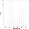 |
Fig. 1 Histogram showing the distribution of program stars as a function of spectral type. |
All the spectra of our program stars have been acquired with the 91-cm telescope and FRESCO, the fiber-fed REOSC echelle spectrograph that allows spectra to be obtained in the range of 4300−6800 Å with a resolution R = 21 000. The spectra were recorded on a thinned, back-illuminated (SITE) CCD with 1024 × 1024 pixels of 24 μm size, whose typical readout noise is of about 8 e− and the gain is 2.5 e−/ADU. All the spectra have been acquired during several observing runs spanning two years between 2008 and 2009.
The reduction of spectra, which included the subtraction of the bias frame, trimming, correcting for the flat-field and the scattered light, the extraction of the orders, and the wavelength calibration, was done by using the NOAO/IRAF package2. The amount of scattered light correction was about 10 ADU. After dividing the extracted spectra by flat-field, the residual shape the spectrum was removed by dividing each spectral order by a Legendre function of a low order. Typical S/N of our spectra is ~100. For some stars this limit has not been reached because its apparent magnitude is close to V ≈ 7, in which case the S/N was about 50.
Adopted astrophysical quantities for our stars and final best-fit parameters.
Finally, the IRAF package rvcorrect was used to include the velocity correction due to the Earth’s motion, which moved the spectra into the heliocentric rest frame. The task splot and its facilities were used to measure the peaks separation in the Hα profile. Errors in the pixels position were converted in errors on the separations, and were evaluated in ≈ 20 km s-1.
For each spectrum we measured the equivalent widths (including underlying absorption) of both Hα and Hβ, where a negative value means the corresponding line shows net emission. All the measured equivalent widths are reported in Table B.1.
3. Classification and fit of the Hα line profiles
Almost all the stars in our sample were found with emission in the Hα. Then, considering the shape of their profile and according to the classification scheme proposed by Hanuschik (1988), we classified our stars as belonging to
-
class 1 when they exhibit a rather symmetricaldouble peak structure with V/R ≈ 1;
-
class 2 when they have an asymmetric single peak or a dominant peak with a much weaker secondary peaked;
-
shell stars when the central reverse is deeper than the continuum level;
-
abs when there is not emission above the continuum level.
Our classification is reported in the fourth column of Table 2.
Only for the stars belonging to class 1, plus stars from other classes but with V/R ratio close to unity, we attempt an estimation of the disk dimension. The approach we used was to minimize the difference between observed and synthetic profiles, computed in two separate steps. First of all, we calculated the photospheric Hα, then the contribution due to the net emission of the disk and then we added these two synthetic profiles obtained separately. These two steps are described in the following:
Computation of the photospheric profile. We first computed the photospheric Hα profiles for all our program stars. They were generated in three steps: i) first, we computed an LTE model atmosphere using the ATLAS9 code (Kurucz 1993); ii) the stellar spectrum was then synthesized using SYNTHE (Kurucz & Avrett 1981); and iii) the spectrum was convolved with the instrumental and rotational profiles. First of all we had to obtain an estimation of the effective temperature for each target. Considering that the continuum energy distribution of Be stars is typical of normal early-type stars both in the visual and UV, but not in the IR, where an excess could be present because of the hot circumstellar dust (Zickgraf 2000), effective temperatures were computed from Strömgren photometry (Hauck & Mermilliod 1998) using the algorithm coded by Moon (1985), with the exception of eight stars for which photometry is not available. This method is allowed because it does not involve any IR filter. For seven of them we adopted the temperatures from the literature: HD 10516, HD 37202, and HD 44458 from Soubiran et al. (2010), HD 58020 and HD 71072 from Hohle et al. (2010), HD 162428 from Moujtahid et al. (1999), and HD 212571 from Wu et al. (2011), while for HD 53416 we derived an estimation of temperature from spectral type and the calibration by Kenyon & Hartman (1995). Since our targets have luminosity class IV/V (as reported in the SIMBAD database), we fixed the surface gravity to log g = 4.0, except for HD 11415, HD 37490, HD 45542, HD 50658, HD 109387, HD 193911, and HD 217050 (luminosity class III) for which log g = 3.0 has been preferred. Radii and masses were adopted following the calibration in Drilling & Landolt (1999). Assuming these atmospheric parameters, we computed the vsini of each star by spectral synthesis of the observed Mgi λ4481 Å. This line was chosen because in the spectral range of our targets, it reaches its maximum depth and therefore it is better suited to determining the rotational velocity. Errors on the projected rotational velocities are ≈ 15 km s-1.
Computation of net disk emission. We have adopted the Be disk model approach of Hummel & Vrancken (2000) that is based on models developed by Horne & Marsh (1986) and Horne (1995) for accretion disks in cataclysmic variables. The disk is assumed to be axisymmetric and centered over the equator of the underlying star, and the gas density varies as
![Mathematical equation: \begin{displaymath} \rho(R,Z)\,=\,\rho_0R^{-n} \exp\left[-\frac{1}{2}\left(\frac{Z}{H(R)}\right)^2\right] \end{displaymath}](/articles/aa/full_html/2013/02/aa20357-12/aa20357-12-eq62.png) where R and Z are the radial and vertical cylindrical coordinates (in units of stellar radii), ρ0 is the base density at the stellar equator, n a radial density exponent, and H(R) the disk vertical scale height. The neutral hydrogen population within the disk is found by equating the photo-ionization and recombination rates (Gies et al. 2007). The disk gas is assumed to be isothermal and related to the stellar effective temperature Teff by Td = 0.6 Teff (Carciofi & Bjorkman 2006). This approach take the contribution of the central star’s finite size on the Hα line formation process into account, i.e. the obscuration of the disk by the central star at any given inclination. The numerical model represents the disk by a large grid of azimuthal and radial surface elements, and the equation of transfer is solved along a ray through the center of each element according to
where R and Z are the radial and vertical cylindrical coordinates (in units of stellar radii), ρ0 is the base density at the stellar equator, n a radial density exponent, and H(R) the disk vertical scale height. The neutral hydrogen population within the disk is found by equating the photo-ionization and recombination rates (Gies et al. 2007). The disk gas is assumed to be isothermal and related to the stellar effective temperature Teff by Td = 0.6 Teff (Carciofi & Bjorkman 2006). This approach take the contribution of the central star’s finite size on the Hα line formation process into account, i.e. the obscuration of the disk by the central star at any given inclination. The numerical model represents the disk by a large grid of azimuthal and radial surface elements, and the equation of transfer is solved along a ray through the center of each element according to 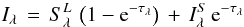 where Iλ is the derived specific intensity, S
 the source function for the disk gas (taken as the Planck function for the disk temperature Td),
  the specific intensity for the Hα of the star, and τλ the integrated optical depth along the ray. The first term applies to all the disk area elements that are unocculted by the star, while the second term applies to all elements that correspond to the projected photospheric disk of the star. The absorption line adopted in
  is Doppler-shifted according to solid-body rotation for the photospheric position in a star that is rotating at 80% of the critical value. Electron scattering is not taken into account in the line profile computation. So we do not expect to reproduce the wings of strong lines well, since for these lines the broadening of the wings due to the electron scattering can not be neglected. Disk kinematic is taken into account using a rotational velocity law written as
  (Hutchings 1970), where R represents the radial coordinate that has its origin at the center of the star, and
  denotes the actual rotational velocity at the stellar surface. The exponent ranges from j = 1/2 for pure Keplerian rotation and j = 1 corresponding to conservation of angular momentum. Likewise the value of j is still matter of debate, recent studies seem to converge toward the Keplerian value (Hummel & Vrancken 2000; Meilland et al. 2007). Thus, in this study we assumed the disk to be in pure Keplerian rotation.
 where N is the total number of points, Iobs and Ith are the intensities of the observed and computed profiles, respectively, and δIobs is the photon noise.
As initial guesses for the inclination angle i and for the disk radius, we used the equations  (1)where veqsini is the value measured in our spectra, and
  (2)(Eq. (6) in Hanuschik et al. 1988) where Δvpeak is the separation between violet and red peaks, as measured in each profile and reported in Table 2.
Then, fine tuning was carried out using the amoeba minimization3 algorithm between observed and computed profiles. In our procedure two assumptions have been made: radial density exponent has been fixed to n = 3 and, as stated before, the Keplerian rotation of the disk has been considered (j = 1/2). The first hypothesis, regarding the value of the density exponent can be justified by considering the work of Grundstrom & Gies (2006). These authors computed several theoretical curves that described the dimension of the disk radius as a function of the Hα equivalent width, for different values of the inclination angle i and different values of n. They concluded that the overall shape of those curves for different n and equal i are almost the same, since it is a small difference of ≈ 3% in correspondence of equivalent widths between − 2 and − 15 Å when n change from 3 to 3.5. They then suggest that the particular choice of n is not as important as the choice of the right i. Moreover, Porter & Rivinius (2003) from IR flux excess in Be stars suggested that n falls in the interval n = 2 ÷ 4. Thus, on the basis of these results, we fixed the value of the density exponent to the middle value of n = 3. Total Hα profiles, star+disk, are presented in Fig. A.1.
To derive an estimation of the disk radius, we used the method developed by Grundstrom & Gies (2006) to form a synthetic image of the system star+disk in the plane of sky by summing the intensity over a 2.8 nm band centered on Hα. We collapsed this image along the projected major axis to get the summed spatial intensity, and we adopted the value for which the summed intensity drops to half its maximum value as effective disk radius.
We estimated the errors on the disk dimensions and on the inclination angles to be ± 2 R∗ and ± 3°, respectively. These determinations have been estimated by varying in Eqs. (1) and in (2) the observed quantities vsini and peak separation by their experimental errors and considering as uncertainties the semi-amplitude of this variation.
All the adopted and derived parameters are reported in Table 2.
4. Hα and Hβ variability
Usually Be stars display variability in their equivalent width (EW) and/or in their spectral profile.
To find whether a star presents equivalent width variation, we applied to both Hα and Hβ equivalent widths the statistical method called F-test. When more than one observation was present for a given target, we calculated the amplitude of the variation, Δ EW, and the standard deviation of the sample using  where N is the number of points, and the (N − 1) corresponds to the degree of freedom used for the F-test. Having obtained ΔEW and σ, we calculated a simple observable to assess the variability for a given target using a ratio of the form:
  (3)
(3)
This simple ratio represents the number of times that the amplitude of the variation is greater than the standard deviation.
To determine whether or not this number is meaningful and whether the star shows variability, we evaluated the corresponding confidence level; see last column of Table 3. We considered all the stars for which C ≥ 80% as definitively variable (13 stars, that is 41% of the sample), while we cannot say anything for the target with C ≤ 50% (22% of the sample) due to the small number of points. The 37% of the stars, are probably variable but within a confidence level ranging from 50% to 80%. In any case, all the targets show the same behavior in both spectral lines.
Program stars for which we have more than two spectra.
In this atlas we show the full set of our profiles (Hα and Hβ) for the 48 observed stars. In Fig. B.1, we show the Balmer profiles observed for program stars with multiple measurements, In each panel we reported for each profile also the last four digits of the heliocentric julian date of the observation. In some cases to improve the visualization, profiles have been blown up according to ![Mathematical equation: \begin{equation} F'_\lambda = [(F_\lambda - 1) * k] + 1 \end{equation}](/articles/aa/full_html/2013/02/aa20357-12/aa20357-12-eq103.png) (4)where Fλ denotes the observed flux,
(4)where Fλ denotes the observed flux,  the displayed flux, and k is the magnification factor.
In Fig. B.2 we show all the stars for which we collected one spectrum only. Most of the stars have been measured several times during the 2008/2009 period, but only few stars showed significant variations in their spectral profiles. These objects are discussed separately in the following:
HD 37202 – this star has been observed in two nights separated by 205 days. It is clearly visible an increase in flux in the violet peak in both spectral lines, even if it is more evident in Hβ.
HD 41335 – as for the previous object, only two observations have been acquired for this star in a range of 207 days. the star exhibits V/R variations in both lines.
HD 58050 – the triple-peaked structure visible in the Hα observed in the first night is missing in the other two spectra. No features are seen in the Hβ.
HD 109387 – this star was observed for 13 nights in a period spanning 110 days. The top part of the Hα emission profiles shows irregular variability, with back and forth changing from class 2 toward class 1, but no evident sign of day-by-day variability has been observed. No variations have been detected in Hβ double-peaked profile.
HD 142926 – during 110 days this shell star was observed 10 times showing a slight V/R variability in the Hα.
HD 143275 – in the four spectra acquired by us, δ Sco shows important changes in the emission of Hα. The V/R changes over the observational period and it shows a flat core in the first spectrum.
HD 164284 – observed for six times in 536 days, this star exhibits equivalent width variability. The double-peaked emission of the Hα profile decrease with time, although the V/R remains constant and ≈ 1. Also the Hβ shows a change in the shape, since it is the last profile without any peak.
HD 183362 – this star shows an increased emission level on the red side of its profile.
HD 183656 – V/R variability has been observed, both in Hα and in Hβ profiles, in the six spectra acquired in a range of 358 days.
HD 187567 – this star show variability in the Hα profile, and evolves from class 1 toward class 2.
HD 189687 – in the Hα, this star does not show any sign of variability for the first month of observations. In the last spectrum taken after 32 days from the second to last, it starts to show an increase of the flux in the red peak. No Hβ variability has been detected.
HD 191610 – this star shows a gradual increment of the flux in the red peak.
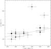 |
Fig. 2 Correlation between measured vsini and peaks separation. The points have been grouped on the basis of the mean equivalent width: EW ≤ –20 Å (filled squares), −20 Å < EW ≤ −15 Å (filled circles), −10 Å < EW ≤ − 5 Å (filled triangles), − 5 Å < EW ≤ 0 Å (open circles), and EW ≥ 0 Å (open squares). |
5. Discussion and conclusions
In this paper we presented a homogeneous sample of Hα and Hβ line profiles observed in 32 Be stars, which show emission at least in the Hα line. According to Hanuschik (1988), we classified our targets on the basis of the following scheme:
-
16 stars, 33% of the sample, in class 1;
-
13 stars, 27% of the sample, in class 2;
-
11 stars, 23% of the total, has been classified as shell stars;
-
6 stars, 12% of the total, do not show net emission.
In this list we do not include the two stars that show any phase transition between classes 1 and 2.
This frequency distribution shows that the majority of our sample of 48 Be stars, randomly distributed in spectral type, belongs to class 1 profiles. Regarding the 13 stars classified as class 2, seven of them are single peak, while six show structured profiles.
Two stars showed variability from one class to another. HD 187567 has undergone an evolution from class 1 to class 2, while the behavior of HD 109387 is more complicated. In 110 days, this star has been observed 13 times, and it showed a transition from class 2 to class 1 and back again to class 2.
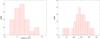 |
Fig. 3 Histograms of distribution of stars as a function of the dimension of their disks (left panel) and of the inclination angles (right panel). To build these histograms we chose a bin size of 2 R∗ and 3°, respectively. |
In Fig. 2 we compared the behavior of the Hα peaks separation to vsini for the stars of the class 1 (included the class 2 HD 60855). A linear correlation seems to exist, as expected from the work of Hanuschik et al. (1988), although two stars discarded from this trend, namely HD 191610 and HD 212571. To verify this correlation we computed the Pearson r coefficient, obtaining r = 0.72 and the linear fit given by the equation:  (5)Thus, we confirm that vsini and Hα peaks separation are in linear correlation, confirming the disk-like geometry of Be star envelopes and, probably this assumption is not valid for HD 191610 and HD 212571.
For all the stars belonging to the class 1, we attempted to model the emission with the purpose of deriving some parameters, such as inclination angle, base density at the stellar equator, and disk radius. In Fig. 3 we show the distribution of stars as a function of the disk radius (right panel) and of the inclination angle (left panel). The histograms were built considering a binning equal to the estimated errors, that is, 2 R∗ and 3° in the disk dimension and inclination angle, respectively. They show there is a major concentration of stars for disks around 6 ÷ 8 R∗ (about 17% of our sample) and for angles around 23° ÷ 35° (about 28% of the sample).
Moreover, with the aim of inferring line profile variability, for most of the stars of our sample we obtained more than one spectrum in a period spanning two years between 2008 and 2009. All but seven stars, those discussed in Sect. 4, do not show any evident sign of variability in both Balmer lines.
IRAF is distributed by the National Optical Astronomy Observatory, which is operated by the Association of Universities for Research in Astronomy, Inc.
The amoeba routine implements the simplex method of Nelder & Mead (1965).
Acknowledgments
This research made use of the SIMBAD database, operated at the CDS, Strasbourg, France.
References
- Carciofi, A. C., & Bjorkman, J. E. 2006, ApJ, 639, 1081 [NASA ADS] [CrossRef] [Google Scholar]
- Drilling, J., & Landolt, A. U. 1999, in Allen’s Astrophysical Quantities, 4th edn., ed. A. N. Cox, Los Alamos, NM [Google Scholar]
- Gies, D. R., Bagnuolo, W. G. Jr., Baines, E. K., et al. 2007, ApJ, 654, 527 [Google Scholar]
- Grundstrom, E. D., & Gies, D. R. 2006, ApJ, 651, 53 [Google Scholar]
- Hanuschik, R. W. 1996, A&A, 308, 170 [NASA ADS] [Google Scholar]
- Hanuschik, R. W., Hummel, W., Sutorius, E., Dietle, O., & Thimm, G., 1996, A&AS, 116, 309 [NASA ADS] [CrossRef] [EDP Sciences] [Google Scholar]
- Hanuschik, R. W., Kozok, J. R., & Kaiser, D. 1988, A&A, 189, 1988 [Google Scholar]
- Hauck, B., & Mermilliod, M. 1998, A&AS, 129, 431 [NASA ADS] [CrossRef] [EDP Sciences] [Google Scholar]
- Hohle, M. M., Neuhauser, R., & Schutz, B. F. 2010, AN, 331, 349 [NASA ADS] [Google Scholar]
- Horne, K. 1995, A&A, 297, 273 [NASA ADS] [Google Scholar]
- Horne, K., & Marsh, T. R. 1986, MNRAS, 218, 761 [NASA ADS] [CrossRef] [Google Scholar]
- Hummel, W., & Vrancken, M. 2000, A&A, 302, 751 [Google Scholar]
- Hutchings, J. B. 1970, MNRAS, 150, 55 [NASA ADS] [Google Scholar]
- Jaschek, M., & Egret, D., 1982, A catalogue of Be stars, In Be stars, eds. M. Jaschek, & H.-G. Groth, Munich, IAU Symp., 98, 261 [Google Scholar]
- Kenyon, S. J., & Hartmann, L. 1995, ApJS, 101, 117 [NASA ADS] [CrossRef] [Google Scholar]
- Kurucz, R. L. 1993, A new opacity-sampling model atmosphere program for arbitrary abundances, in Peculiar versus normal phenomena in A-type and related stars, eds. M. M. Dworetsky, F. Castelli, & R. Faraggiana, IAU Colloq. 138, ASP Conf. Ser., 44, 87 [Google Scholar]
- Kurucz, R. L., & Avrett, E. H. 1981, SAO Spec. Rep., 391 [Google Scholar]
- Meilland, A., Stee, Ph., Vannier, M., et al. 2007, A&A, 464, 59 [Google Scholar]
- Moon, T. T. 1985, Comm. from the Univ. of London Obs., 78 [Google Scholar]
- Moujtahid, A., Zorec, J., & Hubert, A. M. 1999, A&A, 349, 151 [NASA ADS] [Google Scholar]
- Nelder, J. A., & Mead, R. 1965, Comput. J., 7, 308 [CrossRef] [Google Scholar]
- Okazaki, A. T. 1997, A&A, 318, 548 [NASA ADS] [Google Scholar]
- Porter, J. M. 1996, MNRAS, 280, L31 [NASA ADS] [CrossRef] [Google Scholar]
- Porter, J. M., & Rivinius, Th. 2003, PASP, 115, 1153 [NASA ADS] [CrossRef] [Google Scholar]
- Saad, S. M., Kubát, J., Korcáková, D., et al. 2006, A&A, 450, 427 [NASA ADS] [CrossRef] [EDP Sciences] [Google Scholar]
- Silaj, J., Jones, C. E., Tycner, C., Sigut, T. A. A., & Smith, A. D. 2010, ApJS, 187, 228 [NASA ADS] [CrossRef] [Google Scholar]
- Slettebak, A., Collins, G. W., & Truax, R. 1992, ApJS, 81, 335 [NASA ADS] [CrossRef] [Google Scholar]
- Soubiran, C., Le Campion, J.-F., Cayrel De Strobel, G., & Caillo, A. 2010, A&A, 515, A111 [NASA ADS] [CrossRef] [EDP Sciences] [Google Scholar]
- Struve, O. 1931, ApJ, 73, 94 [NASA ADS] [CrossRef] [Google Scholar]
- Wu, Y., Singh, H. P., Prugnel, P., Gupta, R., & Koleva, M. 2011, A&A, 525, A71 [NASA ADS] [CrossRef] [EDP Sciences] [Google Scholar]
- Zickgraf, F.-J. 2000, The connection with B[e] stars, In The Be phenomenon in Early-Type stars, eds. M. A. Smith, H. F. Henrichs, & J. Fabregat, IAU Colloq. 175, ASP Conf. Ser., 214, 26 [Google Scholar]
Appendix A: Fit emission
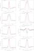 |
Fig. A.1 Observed Hα of Be stars with both stellar absorption (dashed green lines) and total emission profiles (solid red lines) overimposed. Best fit parameters for stellar and disk synthetic profiles are reported in Table 2. The circumstellar emission have been calculated by fixing the radial density exponent (n = 3) and considering Keplerian rotation of the disk (i.e. j = 1/2). |
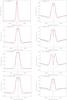 |
Fig. A.1 continued. |
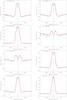 |
Fig. A.1 continued. |
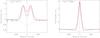 |
Fig. A.1 continued. |
Appendix B: Variability
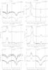 |
Fig. B.1 Line profiles of Hα and Hβ observed for our program stars. Spectra have been shifted along the vertical axis according to the Julian Day of their observation, whose last four digits are reported. In parenthesis we report the magnification factors applied to each profiles in order to improve the visualization. |
 |
Fig. B.1 continued. |
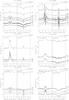 |
Fig. B.1 continued. |
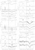 |
Fig. B.1 continued. |
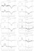 |
Fig. B.1 continued. |
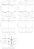 |
Fig. B.1 continued. |
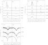 |
Fig. B.2 Hα and Hβ profile for stars for which we only have one spectrum. In the boxes we display shell and class 1 stars, class 2 stars, and stars showing absorption, respectively. |
All Tables
Spectral types, luminosity classes, Strömgren photometry, and derived effective temperatures for our program stars.
All Figures
|
Fig. 1 Histogram showing the distribution of program stars as a function of spectral type. |
| In the text | |
|
Fig. 2 Correlation between measured vsini and peaks separation. The points have been grouped on the basis of the mean equivalent width: EW ≤ –20 Å (filled squares), −20 Å < EW ≤ −15 Å (filled circles), −10 Å < EW ≤ − 5 Å (filled triangles), − 5 Å < EW ≤ 0 Å (open circles), and EW ≥ 0 Å (open squares). |
| In the text | |
|
Fig. 3 Histograms of distribution of stars as a function of the dimension of their disks (left panel) and of the inclination angles (right panel). To build these histograms we chose a bin size of 2 R∗ and 3°, respectively. |
| In the text | |
|
Fig. A.1 Observed Hα of Be stars with both stellar absorption (dashed green lines) and total emission profiles (solid red lines) overimposed. Best fit parameters for stellar and disk synthetic profiles are reported in Table 2. The circumstellar emission have been calculated by fixing the radial density exponent (n = 3) and considering Keplerian rotation of the disk (i.e. j = 1/2). |
| In the text | |
|
Fig. A.1 continued. |
| In the text | |
|
Fig. A.1 continued. |
| In the text | |
|
Fig. A.1 continued. |
| In the text | |
|
Fig. B.1 Line profiles of Hα and Hβ observed for our program stars. Spectra have been shifted along the vertical axis according to the Julian Day of their observation, whose last four digits are reported. In parenthesis we report the magnification factors applied to each profiles in order to improve the visualization. |
| In the text | |
|
Fig. B.1 continued. |
| In the text | |
|
Fig. B.1 continued. |
| In the text | |
|
Fig. B.1 continued. |
| In the text | |
|
Fig. B.1 continued. |
| In the text | |
|
Fig. B.1 continued. |
| In the text | |
|
Fig. B.2 Hα and Hβ profile for stars for which we only have one spectrum. In the boxes we display shell and class 1 stars, class 2 stars, and stars showing absorption, respectively. |
| In the text | |
Current usage metrics show cumulative count of Article Views (full-text article views including HTML views, PDF and ePub downloads, according to the available data) and Abstracts Views on Vision4Press platform.
Data correspond to usage on the plateform after 2015. The current usage metrics is available 48-96 hours after online publication and is updated daily on week days.
Initial download of the metrics may take a while.