| Issue |
A&A
Volume 550, February 2013
|
|
|---|---|---|
| Article Number | A23 | |
| Number of page(s) | 9 | |
| Section | Interstellar and circumstellar matter | |
| DOI | https://doi.org/10.1051/0004-6361/201220341 | |
| Published online | 18 January 2013 | |
HI shells in the Leiden/Argentina/Bonn HI survey⋆
Astronomical Institute, Academy of Sciences, Boční II 1401, Prague, Czech Republic
e-mail: This email address is being protected from spambots. You need JavaScript enabled to view it.
Received: 6 September 2012
Accepted: 9 November 2012
Abstract
Aims. We analyse the all-sky Leiden/Argentina/Bonn HI survey, where we identify shells belonging to the Milky Way.
Methods. We used an identification method based on the search of continuous regions of a low brightness temperature that are compatible with given properties of HI shells.
Results. We found 333 shells in the whole Galaxy. The size distribution of shells in the outer Galaxy is fitted by a power law with the coefficient of 2.6 corresponding to the index 1.8 in the distribution of energy sources. Their surface density decreases exponentially with a scale length of 2.8 kpc. The surface density of shells with radii ≥100 pc in the solar neighbourhood is ~4 kpc-2 and the 2D porosity is ~0.7.
Key words: ISM: bubbles / ISM: general
Tables A.1 and A.2 are only available in electronic form at the CDS via anonymous ftp to cdsarc.u-strasbg.fr (130.79.128.5) or via http://cdsarc.u-strasbg.fr/viz-bin/qcat?J/A+A/550/A23
© ESO, 2013
1. Introduction
The neutral interstellar medium (ISM) in galaxies is full of structures. Some of them are turbulent, wildly changing structures, others are more stable, while HI in particular shows very prominent structures. We see roughly elliptical objects with sizes from a few pc to more than 1 kpc, which may expand into the ambient medium. In the Milky Way they were identified for the first time by Heiles (1979), and since then they have been discovered in many external galaxies, both spiral and irregular, including the Large and Small Magellanic Clouds (for a more complete review see, e.g., Bagetakos et al. 2011).
Shells may be the results of different processes in the ISM. It is a challenge to distinguish between shells created by the energy inserted by stellar winds, stellar radiation, and supernovae explosions; and structures created by other driving mechanisms, such as the infalling high-velocity clouds, gamma ray bursts, or the turbulence driven by galactic differential rotation. Walls of shells may develop Rayleigh-Taylor, Vishniac, Jeans, or other instabilities, thereby creating high-density and low-temperature regions, which become sites of secondary triggered star formation. Dense condensations of cold gas along the edges of shells, secondary star formation, and compact HII regions of second-generation stars have been observed by Zavagno et al. (2006), Deharveng et al. (2010), and others (see also review by Elmegreen 2012). However, many details on the stars vs. shells connection remain unknown, e.g., the number of shells per association, the energetics involved, and the fraction of shells with nonstellar origins.
Due to our position inside the Milky Way, observations of shells in the Galaxy present special problems: unlike observations of external galaxies, an observer has to process a substantial part, ideally all, of the sky to cover the whole Galaxy. The structures do not lie at almost the same distance as in external galaxies, therefore results are more dependent on the distance of objects from the Sun. Another difference is the shape of the shells perpendicular to the galactic symmetry plane. It is directly observable in the Milky Way, while not so clear in external galaxies, where we have to consider the orientation relative to the line of sight. In the Milky Way, there are many observations of individual shells and several papers dealing with the global picture (Heiles 1979; McClure-Griffiths et al. 2002; Daigle et al. 2007; Ehlerová & Palouš 2005), but even these do not cover the whole Galaxy.
Since 2005 the all-sky Leiden/Argentina/Bonn HI survey has been available (LAB; Kalberla et al. 2005). Surveys of the sky available from the Parkes telescope (GASS; Kalberla et al. 2010) and the Effelsberg telescope (EBHIS; Kerp et al. 2011) exist or will exist in the near future and have a higher resolution than LAB. There are other surveys with a higher resolution (the Southern Galactic Plane Survey, the Canadian Galactic Plane Survey, the VLA Galactic Plane Survey), but they cover only the region along the Galactic equator.
Identification of shells is usually done by eye. Human eyes are very good at connecting partially disconnected parts of shells and using some software tools (e.g. some routines in KARMA Gooch 1997) may help. Still, an objective method is preferable. There are a few attempts at an automatic identification process for shells: Thilker et al. (1998) compared a hydrodynamical model with observations; Daigle et al. (2007) based their method on finding simple dynamical characteristics in HI data; and Ehlerová & Palouš (2005, Paper I) located continuous regions of low brightness temperature. The first attempt was not followed any further, probably because it is very difficult to construct a satisfactory and universal hydrodynamical model comparable to the real data. The second approach is aimed at small bubbles (typically ~10 pc) and was used for a portion of the Canadian Galactic Plane Survey data, which found ~7000 bubbles with radii rsh < 40 pc. The third approach is developed in this communication.
2. Data and methods
2.1. Leiden-Argentine-Bonn survey
The Leiden-Argentine-Bonn HI survey (LAB, Kalberla et al. 2005) is an all-sky survey, a combination of the Leiden-Dwingeloo survey (Hartmann & Burton 1997) and the Instituto Argentino de Radioastronomía survey (Bajaja et al. 2005), with angular resolution 36 arcmin (the pixel size 30 arcmin) and velocity resolution 1 km s-1 (the channel width is 1.0306 km s-1). We used the datacube limited in vlsr to ( − 250, + 250) km s-1.
2.2. Identification process
The identification process is divided into three steps: 1) we trace continuous regions around local minima in 2D channel maps; 2) we construct 3D structures from 2D identifications from step 1 by connecting consecutive overlapping regions; 3) we eliminate structures that are not compatible with the given properties of HI shells.
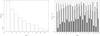 |
Fig. 1 Relative number of structures identified in LAB as a function of their velocity extent (left panel); the relative number of structures that fulfill the P2,min criterion (hatched), P2,ave criterion (cross-hatched), P3 criterion (empty), and all three (solid) as a function of the extent of velocity (right panel). |
2.2.1. Definition of a 2D structure
In channel maps we search for regions with locally low brightness temperatures. The region has to be continuous, i.e. all pixels that belong to it must be connected by their edges, not only by touching their corners, and their brightness temperatures must be lower than or equal to a certain level of brightness temperature TBlevel. All neighbouring pixels, which are not members of the identified region, have to have brightness temperatures higher than TBlevel. These conditions allow embedded clouds with a higher temperature.
For each channel map, the range of TBlevel is examined, starting at a level of noise and growing to the maximum brightness temperature in the map. For the LAB processing we used the square root scale for the brightness temperature (i.e. we worked with  , not directly with TB), the lowest TBlevel we processed was 0.64 K,
  was increased by steps of 0.2.
The identified region has sizes in l and b directions. These sizes have to be within limits (dpixmin, dpixmax). For each region we find the highest TBlevel for which it is fulfilled. We used dpixmin = 3, which eliminated single pixels and very small structures and sets the minimum size of a structure to 1.5°. The value of dpixmax, set to 90 (e.g. 45°), has no clear physical or numerical meaning, but we find out that it gives good results; we were able to identify a whole range of structures under many conditions occurring in the data. A lower value of dpixmax would prevent identification of angularly large shells. Very few 2D structures have sizes larger than dpixmax = 90, only a few identifications in the solar neighbourhood, where such angularly large shells might occur.
2.2.2. Creating a 3D structure
For each 2D region identified in the previous step we check that it has a counterpart in subsequent channel maps. We measure the overlap between the neighbouring 2D structures, and if it is large enough, we connect them in one 3D structure. This continues for all velocity channels and for all structures, until all possible connections are made.
The overlap condition is that at least a fraction p of the area of the smaller one of these two structures is overlapped. We used a value p = 0.5, but results were not very sensitive to this value (we also tested values 0.1 and 0.9). If we use a low value of p, we may artificially connect two or more physically unrelated, but neighbouring, structures, while for a high value of p we may divide one physical structure with an irregular shape into several smaller pieces.
Connecting 2D structures into 3D ones may increase the angular sizes of structures, so they can exceed the value dpixmax.
2.2.3. Properties of HI shells
We do not prescribe any desired shape for an HI shell, we only request that structures, which we call shells, span a certain velocity extent and that their shapes do not change significantly between consecutive velocity channels.
The first condition is simple. We demand that the velocity extent of the structure Δv is greater than a given value. The velocity extent is  (1)where vmin and vmax delimit the interval in which the structure exists.
To estimate how much the shape of the structure changes between the velocity channels we calculate the parameter P2 (2)where Npix(iv) is the number of pixels belonging to the structure in the channel iv, Nboth(iv,iv + 1) is the number of overlapping pixels, i.e. those pixels with positions il, ib, which belong to the structure in both channels iv and iv + 1.
If P2 has a low value, it means that the lb-size or the lb-position in subsequent velocity channels are very different. It may also mean that the 3D shape of the structure changes substantially between the two neighbouring channels. It serves as a warning that the structures might not be compact or uniform. Since an ideal expanding shell, viewed in velocity channels, starts small, reaches its maximum size, and then shrinks again, we determine the average P2,ave and the minimum value P2,min, not in the whole velocity range of the structure, but only in the limited range of velocity channels between the two local maxima in P2, the first after the lowest velocity channel, the second the last before the highest velocity channel.
The calculation of P2 is similar, but not identical, to the calculation of the overlapping parameter p in the previous step. The difference is that 1) here we compare the number of overlapping pixels with the larger of these two channel structures (it was the smaller one previously), and 2) in this step we already evaluate a structure constructed from several originally individual 2D parts.
The spectrum through the centre of the shell should be seen as a noticeable, smooth depression in the brightness temperature profile compared to the profile outside the shell. We construct the relative profile  (3)where Tin is the average brightness temperature in pixels belonging to the structure in a given velocity channel and Tout is the average value of TB in pixels just outside the structure. Which pixels are outside is determined for each velocity channel separately to account for the changing lb-size of the structure. Then we define
  (4)i.e., the maximum difference in average values of brightness temperature inside and outside the shell in all channels where the given structure exists. Clearly visible shells have high P3. Low P3 is connected with poorly visible shells, but also with shells in a region with high TB gradients.
The 3D structure is claimed to be an HI shell if it fulfills the following three conditions:  (5)with a possible auxiliary “visibility” parameter,
  (6)where the values of Δvmin,
  ,
,  , and
, and  determine the strictness of the search.
2.3. A new version of the identifying algorithm
The numerical code described in this paper is a successor to the code described and used in Ehlerová & Palouš (2005). The main differences follow.
-
1.
The current version deals with the whole datacube at once,while the old version had to cut the big datacube into smallersubcubes and then connect them back together. Cutting the big datacube into smaller ones led to artificial edgeproblems (most important to distortions in the shape of identifiedstructures and the failure of some identifications).
-
2.
The last step in the identification, “Properties of HI shells”, was completely changed. The old version used the analysis of the TB(v) spectrum through the central pixel of the structures, the current version used the geometrical parameters P2,min and P2,ave, and an auxiliary visibility parameter P3. Both versions used the condition with the Δvmin, which was set in the previous version to Δvmin = 4 km s-1. The spectrum analysis worked well for small structures in smooth surroundings. For larger structures and a more violent medium, it was sensitive to the exact position of the studied spectrum and to the definition of the background enhancing the possibility of false identifications. Geometrical parameters from the current version are more robust.
3. Results
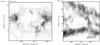 |
Fig. 2 Region of GS242-02+37, one of the expanding shells in Heiles (1979), as seen in the LAB survey. The original identification is shown by the black cross (length of its arms corresponds to published sizes), our new identification (the structure GSH243.5-02.5+043.3 in appended tables) is shown by the box. Left panel is the lb − map, right panel is the lv − diagram. |
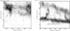 |
Fig. 3 Region of GS228-05+47, one of the stationary shells in Heiles (1979), as seen in the LAB survey. The original identification is shown by the black cross (length of its arms corresponds to published sizes), our new identification (the structure GSH226.5-09.5+031.9 in appended tables) is shown by the box. Left panel is the lb-map, right panel is the lv-diagram. |
3.1. LAB
We used the LAB survey with | vlsr | ≤ 250 km s-1 as an input datacube for our identifying algorithm. Using dpixmin = 3 and dpixmax = 90 as a minimum and a maximum size of the structures and the overlapping parameter p = 0.5, we identified 17535 3D structures. The majority of these structures span only a few velocity channels (see Fig. 1, left panel): 2152 structures (12%) have a velocity extent greater than or equal to four channels (4.1 km s-1), 775 structures (4.4%) have an extent greater than or equal to eight channels (8.2 km s-1). We eliminated irregular structures by adopting parameters  and
and  (see Fig. 1, right panel, showing the fraction of structures, which fulfill the required criteria). Geometrical conditions and eliminate fewer than ~40% of the shells (depends on their velocity extent). As shown in Fig. 1, the most restrictive parameter is the visibility parameter : only about 40 − 50% of shells have parameter P3 greater than 4 K. The value of
  K will be justified in the next section.
The most important criterion in eliminating shells is the minimum required velocity extent Δvmin. The lowest acceptable value is probably Δvmin = 4 km s-1, and the safe option is closer to Δvmin = 8 km s-1. This parameter is related to the dispersion velocity in the ISM. A value of Δvmin lower than the typical velocity dispersion leads to identification of some false structures, while the higher value may eliminate some real structures. The dispersion velocity in ISM varies greatly, depending on the conditions in ISM, but its typical value for the HI emission is around 7 km s-1.
3.2. Comparisons to previously known HI shells
Comparison of identifications with HI supershells: the whole Galaxy (the middle section), the 2nd and 3rd quadrants (the right section).
We compared our LAB identifications to two previous papers on HI shells in the Milky Way: Heiles (1979) and McClure-Griffiths et al. (2002), which contain the majority of known HI supershells. Heiles’s list is divided into two parts: stationary shells, which do not change their size with velocity; and expanding shells, which show different sizes in different velocity channels.
Table 1 shows a comparison of 82 supershells from the two papers with our LAB identifications for the whole datacube (the middle section of the table) and separately for the second and third quadrants (the right section of the table). We chose these two quadrants, because they contained only the outer Galaxy, where structures are less crowded, which makes identifications more accurate. We distinguish whether the shells have similar sizes (“volume restricted”) or not (“volume unrestricted”).
The best agreement was for the McClure-Griffiths shells (in all cases more than 50% of supershells were re-identified), the worst agreement for Heiles’ stationary shells. This is due to the quality of data used in the different searches. Stationary shells were re-identified with different sizes more frequently than expanding shells: the trace of a stationary shell in a datacube is less sharply defined, less pronounced, and not as specific as the trace of an expanding shell, and therefore it is easily mistaken by both human eyes and numerical methods. Figures 2 and 3 show one expanding and one stationary shell from the list by Heiles (1979) and the corresponding LAB identifications. Comparisons in the outer Galaxy were more favourable. This is, we believe, because the ISM in the inner Galaxy is very violent, and there is an overlap from near and far regions along the line of sight, leading to problems in artificial connections of unrelated structures, all of which make identifications in the inner Galaxy less reliable.
We conclude that our method is reliable in the outer Milky Way, because we are able to identify the majority of known expanding HI supershells and a part of known stationary HI supershells again. However, even in the outer Milky Way the existence of some of these published shells is doubtful. Our method is less reliable in the inner Milky Way.
All LAB identifications connected to the previously known HI supershells had Δv ≥ 9 km s-1, P2,min ≥ 0.2, P2,ave ≥ 0.7, and P3 ≥ 4.0 K.
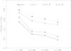 |
Fig. 4 Comparisons between previous and current versions of the search algorithms. Different symbols denote different sets of parameters put on new identifications (see the text for the exact explanation of delv4, C2 |
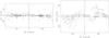 |
Fig. 5 Distribution of 333 identified shells on the sky. Left panel: lb-map; right panel: lv-map. |
3.3. Comparison to the previous version of the search algorithm
The previous version of the search algorithm was applied to the Leiden-Dwingeloo HI survey (only the northern sky, Ehlerová & Palouš 2005). We compared current LAB identifications with our previous identifications. We restricted ourselves to the second quadrant, which was fully observed in the previous version and which did not suffer from shell crowding in the inner Galaxy.
We compared what fraction of shells identified by the previous method (277 in total in the 2nd quadrant) was re-identified by the new method with various values of search parameters Δvmin, P2,ave (the average overlap), P2,min (the minimum overlap), and P3 (visibility parameter). In Fig. 4 we show the comparison for
-
1.
Δvmin = 4 km s-1 (designated as delv4 in Fig. 4, an undemandingcondition);
-
2.
Δvmin = 4 km s-1, P2,min ≥ 0.2, P2,ave ≥ 0.5 (designated C2
 4 in Fig. 4);
 -
3.
Δvmin = 8 km s-1, P2,min ≥ 0.2, P2,ave ≥ 0.5 (designated as C2
8 in Fig. 4); -
4.
Δvmin = 8 km s-1, P2,min ≥ 0.2, P2,ave ≥ 0.5, P3 = 4 K (designated as C3
8 in Fig. 4, the strictest set of conditions).
Furthermore, we demanded that sizes of shells were similar (“volume restricted”). Corresponding fractions were 61% (the 1st set of conditions), 54% (2nd), 33% (3rd), and 26% (4th). Each structure in the previous version had a visual quality, which describes how good it looked (a purely subjective criterion: a shell with q = 1 is clearly visible in velocity channels and is probably spherical or elliptical; a shell with q = 4 is inconspicuous in velocity channels, with a low contrast to its surrounding and probably fragmented and irregular). The comparison was performed separately for shells with different qualities (Fig. 4), and the best-looking shells (visual quality 1) had corresponding fractions ranging from 80% to 55%. Fractions of reidentified shells for volume-unrestricted comparisons were 88% (the 1st set of conditions), 81% (2nd), 76% (3rd), and 72% (4th).
We also compared what fraction of those shells that fulfilled the given set of conditions were also classified as shells by the previous method (Fig. 4). The fractions are 25% for the first set of conditions, 29% (2nd), 48% (3rd), and 74% (4th). That means that three fourths of shells fulfilling the strictest set of conditions were also defined as shells by the previous method. One fourth are new: these shells were rejected because of edge effects inherent to the previous version of the code (described in the Sect. 2.3).
The summary of these results follows. The less strict the set of conditions used for the new identifications, the better the agreement we get with the previous version of the searching algorithm. Visually nice shells are much less sensitive to the precise choice of conditions and methods. Differences arise for the less pronounced and not very regular structures.
By using the fourth set of conditions (Δvmin = 8 km s-1, P2,min ≥ 0.2, P2,ave ≥ 0.5, P3 = 4 K), we chose structures that have regular, not wildly changing shapes that are noticeable and have a large velocity extent. All previously known supershells belong to this group, and the majority of shells from this group were also identified by the previous method. This is the default setting for any further discussion.
4. Discussion
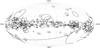 |
Fig. 6 Identified HI shells, Hammer-Aitoff projection, centered on l = 0°, b = 0°. |
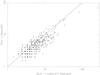 |
Fig. 7 Angular sizes of identified shells. |
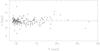 |
Fig. 8 Positions of identified supershells: the galactocentric distance R and the distance from the Galactic plane z. |
4.1. Sky distribution of identified shells
We identify 333 shells in the LAB data, which fulfill the following criteria: Δvmin = 8 km s-1 (the minimum velocity span); P2,min ≥ 0.2, P2,ave ≥ 0.5 (geometrical parameters); and P3 = 4 K (the visibility parameter). Their positions on the sky and in velocity space are shown in Figs. 5 and 6. Ellipses in Fig. 6 correspond to sizes of shells. Angular sizes of shells are shown in Fig. 7. The majority of structures are elongated in the l direction rather than in b, which may be explained as a consequence of the lower shell column densities in high b directions.
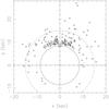 |
Fig. 9 Distribution of supershells in the Galactic plane. The position of the Sun is shown and two circles with galactocentric distances of 8.5 kpc and 15 kpc are overlaid. |
Table A.1, available at the CDS, contains the names and positions of all identified structures: the name with coordinates of the centre; and the minimum and maximum l, b and vlsr, where the structure is visible.
4.2. Galactic distribution of shells
The kinematic distances of identified HI shells are derived using the rotation curve of Brand & Blitz (1993), assuming R⊙ = 8.5 kpc, V⊙ = 220 km s-1. We consider only shells in the outer Galaxy. We exclude shells found at very low velocities | vlsr | < 10 km s-1, since identifications at these low velocities are heavily influenced by the local emission. We also disregard shells close to the centre and anticentre directions (l < 20°, l > 340°, 170° < l < 190°) and shells with very high b coordinates ( | b | > 50°), since noncircular motions may be comparable to projected rotational motions. These selection criteria concern the following analyses and figures from Fig. 8 onwards only.
Table A.2, available at the CDS, contains the following information about these shells: the galactocentric distance R, the radius of the shell rsh (calculated as a geometrical mean of sizes in l and b directions), the expansion velocity vexp (calculated as half of the measured velocity extent), the estimated energy input L needed to create the shell based on the solution of Weaver et al. (1977), assuming the density from Kalberla & Dedes (2008), and the approximate age of the shell texp (based on the solution of Weaver et al. 1977).
Figures 8 and 9 show galactic coordinates of shells and their positions in the Galactic plane. At galactocentric distances greater than 19 kpc, there are shells only in the second quadrant, others are nearly empty. This is especially striking for the third quadrant, which is, from the geometrical point of view, equivalent to the second one.
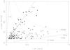 |
Fig. 10 rv diagram of supershells. Evolutionary lines (Weaver et al. 1977) for three luminosities are overlaid (dotted lines), as well as three lines of different times (dashed lines), for the density n0 = 0.3 cm-3. Different symbols denote estimated energy inputs to shells, when densities from Kalberla & Dedes (2008) are taken into account (see text for the explanation): crosses for L < 0.1 SN Myr-1, open circles for 0.1 SN Myr-1 ≤ L ≤ 1.0 SN Myr-1, triangles for L > 1.0 SN Myr-1. |
Figure 10 shows the rv diagram, i.e. the dependence of the expansion velocity of the shell on its radius. The expansion velocity of the shell is calculated as 0.5Δv, and the radius is the geometric mean of sizes in l and b directions. Using the analytical solution for the shell evolution (Weaver et al. 1977), we derive the required energy inputs for individual shells and their ages, using the density based on the distribution of Kalberla & Dedes (2008) and the warp parameters of Levine et al. (2006). We find that 11 shells require energy inputs higher than ~1 SN Myr-1. Calculated energy inputs are given by different symbols in Fig. 10.
The analytical solution (Weaver et al. 1977, lines in Fig. 10) is overlaid for three different luminosities (0.1 SN Myr-1, 1.0 SN Myr-1, 10.0 SN Myr-1), assuming the ISM density n0 = 0.3 cm-3 (which is an overestimate for the majority of shells) and for three different evolutionary times (1 Myr, 10 Myr, and 100 Myr). This solution serves as a guideline, especially for ages, since the evolutionary age in Weaver et al. (1977) does not depend on density and luminosity, while the calculated luminosity depends linearly on the density. We detect a few shells with ages below 5 Myr, which is given by the resolution of the survey and constraints on the sizes. There is only one shell with age greater than 100 Myr. This lack of old shells may be explained by dissolution due to random motions and turbulence or due to destruction by spiral arms, differential rotation, and other galactic forces.
4.2.1. Size distribution of shells
We assume a power-law distribution for sizes of shells 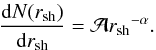 (7)We can then calculate the average size of shells
  at a given heliocentric distance dhc using observed minimum and maximum sizes rmin(dhc) and rmax(dhc):
  (8)Since we restrict the minimum and maximum angular size on identified shells, rmin and rmax must depend on the distance (see Fig. 11, left panel). With known or assumed
  , rmin, and rmax (assumptions are connected to restrictions on angular sizes of detected structures), we can calculate α. Solutions lie in the interval (2.2, 3.1), the best solution is for 2.6. This value might be artificially flatter than the real value, since our identifying algorithm forms one big shell from two small shells more frequently than vice versa, producing a flatter size spectrum.
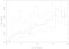 |
Fig. 11 Dependence of minimum (dash-dotted line), average (solid line), and maximum (dashed line) radius of the shell rsh as a function of the heliocentric distance dhc. |
An alternative method to calculate the coefficient α, used in Paper I, is to take such a subset of identified shells, which in a certain range of distances contains shells in a given range of sizes. Results of this method cover an interval of α and include the value 2.6 calculated here. Uncertainties in the determination of α are fairly large, probably because our identifying algorithm is better at localizing structures than at determining their precise sizes.
The average value of α in external galaxies (Bagetakos et al. 2011) is 2.9, which is a slightly steeper value than ours. Their value is an average through several types of galaxies and there is a dependence of the coefficient α on the galaxy type (early type spirals tend to have steeper slopes). According to their Fig. 28, our value of 2.6 corresponds to Sc galaxies.
The coefficient α is connected to the power-law coefficient β of the luminosity function of sources creating shells, e.g. OB associations 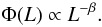 (9)According to Oey & Clarke (1997)α and β are connected as
  (10)Therefore, β ~ 1.8, which is somewhat flatter than the expected luminosity function of OB associations in the Milky Way (2.0; see e.g. McKee & Williams 1997).
4.2.2. Radial distribution of shells
We assume that the shell surface density follows an exponential distribution 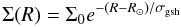 (11)where Σ(R) is the surface density of HI shells.
Typical sizes of shells, hence the relative proportion of identified to total number of shells, change with heliocentric distance, and therefore to get intrinsic values of Σ(R) we have to correct the observed values. With the corrected value we can calculate σgsh. We apply the same method as in Paper I, briefly described in the Sect. 4.2.1. It is based on selecting subsets that contain information for a chosen interval of heliocentric distances and sizes. The radial distribution of the shell surface density Σ(R) is based on the number of shells with the galactocentric distance R corrected for the limitations caused by a finite range of heliocentric distances. Results depend on the selected interval of distances, but in a particular way: results, which are consistent with the assumed exponential decrease (i.e. show a high correlation between observed numbers of shells with numbers predicted from Eq. (11)) form a distinct group, while the others form another one with a wide spread in values of σgsh. Good solutions for σgsh have the average value of (2.8 ± 0.5) kpc.
After extrapolating solutions for the size distribution of shells and the radial dependence of the shell surface density, we can estimate the total number of shells and also the porosity of the Galaxy. These extrapolations are not too precise, since they combine all inaccuracies coming from errors in the derivation of α and σgsh, and they also include the effect of selection criteria described in the Sect. 3. Taking the minimum size of a shell to be 100 pc and the maximum size to be 1 kpc, we come to the conclusion that there should be something like 400 to 1000 shells in the outer Galaxy, and about 2000 to 5000 such shells in the whole Galaxy.
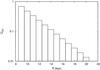 |
Fig. 12 2D porosity of the outer Milky Way. |
The number surface density of HI shells with radii rsh ≥ 100 pc in the solar neighbourhood is about  shells per kpc2. Apart from uncertainties connected with extrapolating, there are intrinsic variations in the surface density (see e.g. Fig. 9), most probably connected to spiral arms. The derived value of surface density is higher than – though not incomparable to – the average value of the same quantity for a number of external galaxies (THINGS galaxies, Bagetakos et al. 2011). The typical value is (0.1 − 1) shells per kpc2, though there are some galaxies in that paper that reach higher values. This discrepancy may be caused by either the less strict conditions put on the identification method for HI shells on our side and stricter conditions on theirs (among others, Bagetakos et al. (2011) demanded quite a high temperature contrast for their shells and regular elliptical shapes), or by a different point of view: from inside in the Milky Way and from outside for external galaxies. The inside view is much more sensitive to shells that did not yet break through the HI disc. On the other hand, the surface density of OB associations in the solar neighbourhood is about 7 per kpc2 (McKee & Williams 1997), which is comparable to our value: we would instead expect a higher number of shells than OB associations, since the typical lifetime of a shell is longer than for an OB association, but clustering of OB associations may decrease the number of OB associations per shell.
The porosity Q, which is a ratio of the surface occupied by shells to the total surface (the 2D porosity) or the volume occupied by shells to the total volume (the 3D porosity), is derived. In the inner Galaxy the porosity as calculated from derived distributions, is large, much larger than 1, which predicts the significant overlapping of shells. The porosity of the outer Galaxy is smaller (see Fig. 12), where values lower than ~0.01 are reached at galactocentric distances of ~20 kpc. Local values at the solar neighbourhood are Q2D = 0.7 and Q3D = 0.4 (assuming a cylinder with height 1 kpc) for shells with radii rsh ∈ (0.1,1.0) kpc. Error boxes are similar to those in the case of number surface density. Porosity (especially Q3D) is mostly dependent on the maximum size of the shell, which we assume to be 1 kpc, and therefore values quoted here approach the real values, since the contribution of small bubbles is negligible.
Daigle et al. (2007) calculate the partial porosity of shells with radii rsh ∈ (5,40) pc in the region of the Perseus arm  . We can do the same thing by extrapolating our solutions to small shells and get the result Q3D = 0.003. This is surprisingly good agreement. If this is not a coincidence, it means that we both detect the same type of objects – in different evolutionary phases – even though we use substantially different approaches. Our somewhat lower value could mean that some of the small objects will not evolve into large structures (such as bubbles created by single supernova explosions).
5. Conclusions
We have identified 333 HI shells in the Leiden/Argentina/Bonn HI survey of the Milky Way using an automatic searching algorithm. The advantage of this approach is the uniformity of conditions throughout the Milky Way. Our method is quite sensitive for locating “something interesting”, while it is not as effective for measuring the precise sizes of the shells.
We discovered the asymmetry between the second and third Galactic quadrants in the distribution of shells at large galactocentric distances. At distances greater than 19 kpc there are shells only in the second quadrant. The third quadrant, which is an equivalent to the second one from the geometrical point of view, contains no shells at these galactocentric distances.
Because of crowding and distance ambiguity in the Milky Way, we base the following conclusions on shells in the outer Galaxy. We found that their radial distribution decreases exponentially on a scale length of 2.8 kpc, and their size distribution is a power law with the coefficient of ~2.6 (corresponding to a power-law coefficient of the luminosity function of OB associations ~1.8). The surface density of shells with radii ⟨ 0.1,1.0 ⟩ kpc in the solar neighbourhood is ~4 kpc-2.
Acknowledgments
This study has been supported by the Czech Science Foundation grant 209/12/1795 and by the project RVO: 67985815. This research made use of NASA’s Astrophysics Data System. The authors would like to thank the anonymous referee for helpful proposals and Jim Dale and the A&A language editor Joli Adams for the help with the manuscript (any remaining inelegance is purely our own).
References
- Bagetakos, I., Brinks, E., Walter, F., et al. 2011, AJ, 141, 23 [NASA ADS] [CrossRef] [Google Scholar]
- Bajaja, E., Arnal, E. M., Larrarte, J. J., et al. 2005, A&A, 440, 767 [NASA ADS] [CrossRef] [EDP Sciences] [Google Scholar]
- Brand, J., & Blitz, L. 1993, A&A, 275, 67 [NASA ADS] [Google Scholar]
- Daigle, A., Joncas, G., & Parizeau, M. 2007, ApJ, 661, 285 [NASA ADS] [CrossRef] [Google Scholar]
- Deharveng, L., Schuller, F., Anderson, L. D., et al. 2010, A&A, 523, A6 [NASA ADS] [CrossRef] [EDP Sciences] [Google Scholar]
- Ehlerová, S., & Palouš, J. 2005, A&A, 437, 101 (Paper I) [NASA ADS] [CrossRef] [EDP Sciences] [Google Scholar]
- Elmegreen, B. G. 2012, IAU Symp., 284, 317 [NASA ADS] [Google Scholar]
- Gooch, R. E. 1997, PASA, 14, 106 [Google Scholar]
- Hartmann, D., & Burton, W. B. 1997, Atlas of Galactic Neutral Hydrogen [Google Scholar]
- Heiles, C. 1979, ApJ, 229, 533 [NASA ADS] [CrossRef] [Google Scholar]
- Kalberla, P. M. W., & Dedes, L. 2008, A&A, 487, 951 [NASA ADS] [CrossRef] [EDP Sciences] [Google Scholar]
- Kalberla, P. M. W., Burton, W. B., Hartmann, D., et al. 2005, A&A, 440, 775 [NASA ADS] [CrossRef] [EDP Sciences] [Google Scholar]
- Kalberla, P. M. W., McClure-Griffiths, N. M., Pisano, D. J., et al. 2010, A&A, 521, A17 [NASA ADS] [CrossRef] [EDP Sciences] [Google Scholar]
- Kerp, J., Winkel, B., Ben Bekhti, N., Flöer, L., & Kalberla, P. M. W. 2011, Astron. Nachr., 332, 637 [NASA ADS] [CrossRef] [Google Scholar]
- Levine, E. S., Blitz, L., & Heiles, C. 2006, ApJ, 643, 881 [NASA ADS] [CrossRef] [Google Scholar]
- McClure-Griffiths, N. M., Dickey, J. M., Gaensler, B. M., & Green, A. J. 2002, ApJ, 578, 176 [NASA ADS] [CrossRef] [Google Scholar]
- McKee, C. F., & Williams, J. P. 1997, ApJ, 476, 144 [NASA ADS] [CrossRef] [Google Scholar]
- Oey, M. S., & Clarke, C. J. 1997, MNRAS, 289, 570 [NASA ADS] [CrossRef] [Google Scholar]
- Thilker, D. A., Braun, R., & Walterbos, R. M. 1998, A&A, 332, 429 [NASA ADS] [Google Scholar]
- Weaver, R., McCray, R., Castor, J., Shapiro, P., & Moore, R. 1977, ApJ, 218, 377 [NASA ADS] [CrossRef] [Google Scholar]
- Zavagno, A., Deharveng, L., Comerón, F., et al. 2006, A&A, 446, 171 [NASA ADS] [CrossRef] [EDP Sciences] [Google Scholar]
Appendix A: Tables
Table A.1 contains observed properties of HI shells. Co-lumn 1 is a running number of the structure, Col. 2 is the name
of structure (GSH + galactic coordinates of the centre and the radial velocity). The remaining columns describe the ranges in coordinates, where the structure is visible: Cols. 3 and 4 the longitude, Cols. 5 and 6 the latitude, Cols. 7 and 8 the radial velocity.
Table A.2 contains derived properties of HI shells. Column 1 is a running number of the structure, Col. 2 is the name of the structure (GSH + galactic coordinates of the centre and the radial velocity). Column 3 is the galactocentric distance of the structure (using the rotation curve of Brand & Blitz 1993), Col. 4 is the radius of the shell (calculated as the geometric mean of dimensions in l and b), Col. 5 is the expansion velocity (calculated as a half of the velocity extent of the structure). Columns 6 and 7 are estimates of the needed energy input into the shell and the evolutionary time based on the model of Weaver et al. (1977). Shells in the inner Galaxy are excluded from this table, as are shells found at very low velocities | vlsr | < 10 km s-1, shells close to the centre and anticentre directions (l < 20°, l > 340°, 170° < l < 190°), and shells with very high b coordinates ( | b | > 50°).
All Tables
Comparison of identifications with HI supershells: the whole Galaxy (the middle section), the 2nd and 3rd quadrants (the right section).
All Figures
|
Fig. 1 Relative number of structures identified in LAB as a function of their velocity extent (left panel); the relative number of structures that fulfill the P2,min criterion (hatched), P2,ave criterion (cross-hatched), P3 criterion (empty), and all three (solid) as a function of the extent of velocity (right panel). |
| In the text | |
|
Fig. 2 Region of GS242-02+37, one of the expanding shells in Heiles (1979), as seen in the LAB survey. The original identification is shown by the black cross (length of its arms corresponds to published sizes), our new identification (the structure GSH243.5-02.5+043.3 in appended tables) is shown by the box. Left panel is the lb − map, right panel is the lv − diagram. |
| In the text | |
|
Fig. 3 Region of GS228-05+47, one of the stationary shells in Heiles (1979), as seen in the LAB survey. The original identification is shown by the black cross (length of its arms corresponds to published sizes), our new identification (the structure GSH226.5-09.5+031.9 in appended tables) is shown by the box. Left panel is the lb-map, right panel is the lv-diagram. |
| In the text | |
|
Fig. 4 Comparisons between previous and current versions of the search algorithms. Different symbols denote different sets of parameters put on new identifications (see the text for the exact explanation of delv4, C2 |
| In the text | |
|
Fig. 5 Distribution of 333 identified shells on the sky. Left panel: lb-map; right panel: lv-map. |
| In the text | |
|
Fig. 6 Identified HI shells, Hammer-Aitoff projection, centered on l = 0°, b = 0°. |
| In the text | |
|
Fig. 7 Angular sizes of identified shells. |
| In the text | |
|
Fig. 8 Positions of identified supershells: the galactocentric distance R and the distance from the Galactic plane z. |
| In the text | |
|
Fig. 9 Distribution of supershells in the Galactic plane. The position of the Sun is shown and two circles with galactocentric distances of 8.5 kpc and 15 kpc are overlaid. |
| In the text | |
|
Fig. 10 rv diagram of supershells. Evolutionary lines (Weaver et al. 1977) for three luminosities are overlaid (dotted lines), as well as three lines of different times (dashed lines), for the density n0 = 0.3 cm-3. Different symbols denote estimated energy inputs to shells, when densities from Kalberla & Dedes (2008) are taken into account (see text for the explanation): crosses for L < 0.1 SN Myr-1, open circles for 0.1 SN Myr-1 ≤ L ≤ 1.0 SN Myr-1, triangles for L > 1.0 SN Myr-1. |
| In the text | |
|
Fig. 11 Dependence of minimum (dash-dotted line), average (solid line), and maximum (dashed line) radius of the shell rsh as a function of the heliocentric distance dhc. |
| In the text | |
|
Fig. 12 2D porosity of the outer Milky Way. |
| In the text | |
Current usage metrics show cumulative count of Article Views (full-text article views including HTML views, PDF and ePub downloads, according to the available data) and Abstracts Views on Vision4Press platform.
Data correspond to usage on the plateform after 2015. The current usage metrics is available 48-96 hours after online publication and is updated daily on week days.
Initial download of the metrics may take a while.