| Issue |
A&A
Volume 550, February 2013
|
|
|---|---|---|
| Article Number | A15 | |
| Number of page(s) | 10 | |
| Section | Numerical methods and codes | |
| DOI | https://doi.org/10.1051/0004-6361/201220332 | |
| Published online | 21 January 2013 | |
Low-ℓ CMB analysis and inpainting
1
Laboratoire AIM, UMR CEA-CNRS-Paris 7, Irfu, Service d’Astrophysique, CEA
Saclay,
91191
Gif-sur-Yvette Cedex,
France
e-mail: This email address is being protected from spambots. You need JavaScript enabled to view it.
2
GREYC CNRS-ENSICAEN-Université de Caen,
6 Bd du Maréchal
Juin, 14050
Caen Cedex,
France
3
Laboratoire d’Astrophysique, École Polytechnique Fédérale de
Lausanne (EPFL), Observatoire de Sauverny, 1290
Versoix,
Switzerland
Received:
4
September
2012
Accepted:
26
October
2012
Abstract
Reconstructing the cosmic microwave background (CMB) in the Galactic plane is extremely difficult due to the dominant foreground emissions such as dust, free-free or synchrotron. For cosmological studies, the standard approach consists in masking this area where the reconstruction is insufficient. This leads to difficulties for the statistical analysis of the CMB map, especially at very large scales (to study for instance the low quadrupole, integrated Sachs Wolfe effect, axis of evil, etc.). We investigate how well some inpainting techniques can recover the low-ℓ spherical harmonic coefficients. We introduce three new inpainting techniques based on three different kinds of priors: sparsity, energy, and isotropy, which we compare. We show that sparsity and energy priors can lead to extremely high-quality reconstruction, within 1% of the cosmic variance for a mask with a sky coverage larger than 80%.
Key words: methods: data analysis / techniques: image processing / cosmic background radiation
© ESO, 2013
1. Introduction
Because component separation methods do not provide good estimates of the cosmic microwave background (CMB) in the Galactic plane and at locations of point sources, the standard approach for a CMB map analysis is to consider that the data are not reliable in these areas, and to mask them. This leads to an incomplete coverage of the sky that has to be handled properly for the subsequent analysis. This is especially true for analysis methods that operate in the spherical harmonic domain where localization is lost and full-sky coverage is assumed. For power spectrum estimations, methods such as MASTER (Hivon et al. 2002) solve a linear ill-posed inverse problem that allows to deconvolve the observed power spectrum of the masked map from the mask effect.
For a non-Gaussianity analysis, many approaches to deal with this missing data problem have been proposed. Methods to solve this problems are called gap-filling or inpainting methods.
The simplest approach is to set the pixel values in the masked area to zero. This is sometimes claimed to be a good approach by assuming it does not add any information. However, this is not correct, as setting the masked area to zero actually adds (or removes) information, which again differs from the true CMB values. A consequence of this gap-filling technique is the creation of many artificial high amplitude coefficients at the border of the mask in a wavelet analysis or a leakage between different multipoles in a spherical harmonic analysis. This effect can be reduced with an apodized mask. A slightly more sophisticated method consists of replacing each missing pixel by the average of its neighbors and iterating until the gaps are filled. This technique is called diffuse inpainting and has been used in Planck-LFI data pre-processing Zacchei et al. (2011). It is acceptable for treatment of point sources, but is far from being a reasonable solution for the Galactic plane inpainting in a CMB non-Gaussianity analysis.
In Abrial et al. (2007; 2008), the problem was considered as an ill-posed inverse problem, z = Mx, where x is the unknown CMB, M is the masking operator, and z the masked CMB map. A sparsity prior in the spherical harmonic domain was used to regularize the problem. This sparsity-based inpainting approach has been successfully used for two different CMB studies, the CMB weak-lensing on Planck simulated data (Perotto et al. 2010; Plaszczynski et al. 2012), and the analysis of the integrated Sachs-Wolfe effect (ISW) on WMAP data (Dupé et al. 2011). In both cases, the authors showed from Monte-Carlo simulations that the statistics derived from the inpainted maps can be trusted at a high confidence level, and that sparsity-based inpainting can indeed provide an easy and effective solution to the large Galactic mask problem.
It was also shown that sparse inpainting is useful for weak-lensing data (Pires et al. 2009), Fermi data (Schmitt et al. 2010), and asteroseismic data (Sato et al. 2010). The sparse inpainting success has motivated the community to investigate more inpainting techniques, and other approaches have recently been proposed.
Bucher & Louis (2012) and Kim et al. (2012) sought a solution that complies with the CMB properties, i.e. to be a homogeneous Gaussian random field with a specific power spectrum. Good results were derived, but the approach presents the drawback that we need to assume a given cosmology, which may not be appropriate for non-Gaussianity studies. For large scale CMB anomaly studies, Feeney et al. (2011) and Ben-David et al. (2012), building upon the work of de Oliveira-Costa & Tegmark (2006), proposed to use generalized least-squares (GLS), which coincide with the maximum-likelihood estimator (MLE) under appropriate assumptions such as Gaussianity. This method also requires an input power spectrum. In addition, when the covariance in the GLS is singular, the authors proposed to regularize it by adding a weak perturbation term that must also to ensure positive-definiteness. With this regularization, the estimator is no longer a GLS (nor a MLE).
Because the missing data problem is ill-posed, prior knowledge is needed to reduce the space of candidate solutions. Methods that handle this problem in the literature assume priors, either explicitly or implicitly. If we exclude the zero-inpainting and the diffuse inpainting methods, which are of little interest for the Galactic plane inpainting, the two other priors are:
-
Gaussianity: the CMB is assumed to be a homogeneous andisotropic Gaussian random field, therefore it is adequate to usesuch a prior. In practice, methods using this prior require thetheoretical power spectrum, which has either to be estimatedusing a method such as TOUSI (Paykariet al. 2012), or a cosmology has tobe assumed, which is an even stronger assumption than theGaussianity prior. We should also keep in mind that the goal ofnon-Gaussianity studies is to check that the observed CMB doesnot deviate from Gaussianity. Therefore, we should be carefulwith this prior.
-
Sparsity: the sparsity prior on a signal consists of assuming that its coefficients in a given representation domain, when sorted in decreasing order of magnitude, exhibit a fast decay rate, typically a polynomial decay with an exponent that depends on the regularity of the signal. Spherical harmonic coefficients of the CMB show a decay in O(ℓ-2) up to ℓ around 900 and then O(ℓ-3) for larger multipoles. Thus, the sparsity prior is advocated, and this explains its success for CMB-related inverse problems such as inpainting or component separation (Bobin et al. 2012).
We here revisit the Gaussianity and sparsity priors, and introduce an additional one, the CMB isotropy, to recover the spherical harmonic coefficients at low ℓ (<10) from masked data. We describe novel and fast algorithms to solve the optimization problems corresponding to each prior. These algorithms originate from the field of non-smooth optimization theory and are efficiently appliedto large-scale data. We then show that some of these inpainting algorithms are very efficient to recover the spherical harmonic coefficients for ℓ < 10 when using the sparsity or energy priors. We also study the reconstruction quality as a function of the sky coverage, and we show that a very good reconstruction quality, within 1% of the cosmic variance, can be reached for a mask with a sky coverage better than 80%.
2. CMB inpainting
2.1. Problem statement
We observe z = Mx, where x is a real-valued centered and square-integrable field on the unit sphere S2, and M is a linear bounded masking operator. The goal is to recover x from z.
The field x can be expanded as
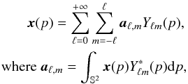 where
the complex-valued functions Yℓm are the
co-called spherical harmonics, ℓ is the multipole moment, and
m is the phase ranging from − ℓ to ℓ.
The aℓ,m are the spherical
harmonic coefficients of x. In the following we will denote
S the spherical harmonic transform operator and S∗
its adjoint (hence its inverse since spherical harmonics form an orthobasis of
L2(S2)).
where
the complex-valued functions Yℓm are the
co-called spherical harmonics, ℓ is the multipole moment, and
m is the phase ranging from − ℓ to ℓ.
The aℓ,m are the spherical
harmonic coefficients of x. In the following we will denote
S the spherical harmonic transform operator and S∗
its adjoint (hence its inverse since spherical harmonics form an orthobasis of
L2(S2)).
If x is a wide-sense stationary (i.e., homogeneous) random
field, the spherical harmonic coefficients are uncorrelated,
 Moreover,
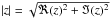
if the process is isotropic, then
Moreover,
if the process is isotropic, then  where
Cℓ is the angular power spectrum, which
depends solely on ℓ.
where
Cℓ is the angular power spectrum, which
depends solely on ℓ.
In the remainder of the paper, we consider a finite-dimensional setting, where the sphere is discretized. x can be rearranged in a column vector in Rn, and similarly for z ∈ Rm, with m < n, and a ∈ Cp. Therefore, M can be seen as a matrix taking values in { 0,1 }, i.e., M ∈ Mm × n({ 0,1 }). The goal of inpainting is to recover x from z.
2.2. a general inpainting framework
The recovery of x from z when m < n amounts to solving an underdetermined system of linear equations. Traditional mathematical reasoning, in fact the fundamental theorem of linear algebra, tells us not to attempt this: there are more unknowns than equations. However, if we have prior information about the underlying field, there are some rigorous results showing that such an inversion might be possible (Starck et al. 2010).
In general, we can write the inpainting problem as the following optimization program
 (1)where R
is a proper lower-bounded penalty function reflecting some prior on
x, and
(1)where R
is a proper lower-bounded penalty function reflecting some prior on
x, and  is closed constraint set expressing the fidelity term. Typically, in the noiseless case,
 .
This is what we focus on in the remainder of the paper. We consider three types of priors,
each corresponding to a specific choice of R.
.
This is what we focus on in the remainder of the paper. We consider three types of priors,
each corresponding to a specific choice of R.
3. Sparsity prior
Sparsity-based inpainting has been proposed for the CMB in (Abrial et al. 2007, 2008) and for weak-lensing mass map reconstruction in Pires et al. (2009, 2010). In Perotto et al. (2010), Dupé et al. (2011) and Rassat et al. (2012), it was shown that sparsity-based inpainting does not destroy CMB weak-lensing, ISW signals or some large-scale anomalies in the CMB, and is therefore an elegant way to handle the masking problem. The masking effect can be thought of as a loss of sparsity in the spherical harmonic domain because the information required to define the map has been spread across the spherical harmonic basis (leakage effect).
Optimization problem
If the spherical harmonic coefficients a of
x (i.e.
a = Sx) are
assumed to be sparse, then a well-known penalty to promote sparsity is the
lq (pseudo- or quasi-)norm, with
q ∈ [0,1]. Therefore, Eq. (1)becomes  (2)where
 , and where
 for z ∈C. For q = 0, the l0
pseudo-norm counts the number of non-zero entries of its argument. The inpainted map is
finally reconstructed as
for z ∈C. For q = 0, the l0
pseudo-norm counts the number of non-zero entries of its argument. The inpainted map is
finally reconstructed as  .
.
Solving Eq. (2)when q = 0 is known to be NP-hard. This is additionaly complicated by the non-smooth constraint term. Iterative Hard thresholding (IHT), described in Appendix A, attempts to solve this problem. It is also well-known that the l1 norm is the tightest convex relaxation (in the ℓ2 ball) of the l0 penalty (Starck et al. 2010). This suggests solving Eq. (2)with q = 1. In this case, the problem is well-posed: it has at least a minimizer, and all minimizers are global. Furthermore, although it is completely non-smooth, it can be solved efficiently with a provably converging algorithm that belongs to the family of proximal splitting schemes (Combettes & Pesquet 2011; Starck et al. 2010). This can be done with the Douglas-Rachford (DR) algorithm described in Appendix B.
Comparison between IHT and DR
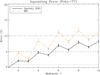 |
Fig. 1 Relative MSE per ℓ in percent for the two sparsity-based inpainting algorithms, IHT (dashed red line) and DR (continuous black line). |
We compared the IHT and DR sparsity-based inpainting algorithms in 100 Monte-Carlo
simulations using a mask with sky coverage Fsky = 77%. In all our experiments, we used 150
iterations for both iterative schemes, β = 1 and
αn ≡ 1 (∀n) in the DR
scheme (see Appendix B). For each inpainted map
i ∈ {1,··· ,100}, we computed the
relative mean squared-error (MSE) ![Mathematical equation: \begin{eqnarray*} e^{(i)}[\ell] = \left< \frac{ \abs{\cmba^{\mathrm{True}}_{\ell,m} - \cmba^{(i)}_{\ell,m} }^2 }{C_{\ell} } \right>_m \end{eqnarray*}](/articles/aa/full_html/2013/02/aa20332-12/aa20332-12-eq54.png) and
the its version in percent per ℓ
and
the its version in percent per ℓ![Mathematical equation: \begin{eqnarray*} E[\ell] = 100 \times \left< e^{(i)}[\ell] \right>_i ~ (\%) . \end{eqnarray*}](/articles/aa/full_html/2013/02/aa20332-12/aa20332-12-eq55.png) Figure
1 depicts the relative MSE in percent per
ℓ for the two sparsity-based inpainting algorithms IHT
(l0) and DR (l1). We see that at
very low ℓ, l1-sparsity inpainting as provided
by the DR algorithm yields better results. We performed the test with other masks and
arrived at similar conclusions. Because we focus on low-ℓ, only the
l1 inpainting as solved by the DR algorithm is considered
below.
Figure
1 depicts the relative MSE in percent per
ℓ for the two sparsity-based inpainting algorithms IHT
(l0) and DR (l1). We see that at
very low ℓ, l1-sparsity inpainting as provided
by the DR algorithm yields better results. We performed the test with other masks and
arrived at similar conclusions. Because we focus on low-ℓ, only the
l1 inpainting as solved by the DR algorithm is considered
below.
4. Energy prior
Optimization problem
If we know a priori the power-spectrum
(Cℓ,m)ℓ,m (not
the angular one, which implicitly assumes isotropy) of the Gaussian field
x, then using a maximum a posteriori (MAP) argument, the
inpainting problem amounts to minimizing a weighted ℓ2-norm
subject to a linear constraint 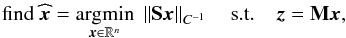 (3)where for a
complex-valued vector a,
(3)where for a
complex-valued vector a,
 ,
i.e. a weighted ℓ2 norm. By strong convexity, Problem Eq. (3)is well-posed and has exactly one minimizer,
therefore justifying equality instead of inclusion in the argument of the minimum in Eq.
(3).
,
i.e. a weighted ℓ2 norm. By strong convexity, Problem Eq. (3)is well-posed and has exactly one minimizer,
therefore justifying equality instead of inclusion in the argument of the minimum in Eq.
(3).
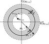 |
Fig. 2 Set Bℓ. |
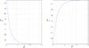 |
Fig. 3 Normalized critical thresholds at the significance level 0.05 as a function of ℓ. |
Since the objective is differentiable with a Lipschitz-continuous gradient, and the projector Proj{ x:z = Mx } on the linear equality set is known in closed-form, one can use a projected gradient-scheme to solve Eq. (3). However, it turns that the estimate of the descent step-size can be rather crude, which may hinder the convergence speed. One can think of using an inexact line-search, but this will complicate the algorithm unnecessarily. This is why we propose a new algorithm in Appendix C, based on the Douglas-Rachford splitting method, which is easy to implement and efficient.
In all our experiments in the remainder of the paper, we used 150 iterations for this
algorithm with β = 50 and
αn ≡ 1 (∀n) (see Appendix C).
This approach requires the power-spectrum Cℓ,m
as an input parameter. In practice, an estimate  of the power spectrum from the data using MASTER was used, and we set
 .
The latter is reminiscent of an isotropy assumption, which is not necessarily true.
.
The latter is reminiscent of an isotropy assumption, which is not necessarily true.
5. Isotropy prior
5.1. Structural constraints on the power spectrum
Strictly speaking, we would define the set of isotropic homogeneous random processes on
the (discrete) sphere as the closed set  where
Cℓ,m = E[|(Sx)ℓ,m|2]
and Cℓ is the angular power spectrum, which
depends solely on ℓ. Given a realization x
of a random field, we can then naively state the orthogonal projection of
x onto
where
Cℓ,m = E[|(Sx)ℓ,m|2]
and Cℓ is the angular power spectrum, which
depends solely on ℓ. Given a realization x
of a random field, we can then naively state the orthogonal projection of
x onto  by solving
  This
formulation of the projection constraint set is not straightforward to deal with for at
least the following reasons: (i) the isotropy constraint set involves the unknown true
Cℓ (through the expectation operator),
which necessitates resorting to stochastic programming; (ii) the constraint set is not
convex.
This
formulation of the projection constraint set is not straightforward to deal with for at
least the following reasons: (i) the isotropy constraint set involves the unknown true
Cℓ (through the expectation operator),
which necessitates resorting to stochastic programming; (ii) the constraint set is not
convex.
5.2. Projection with a deterministic constraint
An alternative to the constraint set
would be to replace Cℓ,m and
Cℓ by their empirical sample estimates,
i.e., Cℓ,m by
|aℓ,m|2 and
Cℓ by
 . However, this
hard constraint might be too strict in practice and we propose to make it softer by taking
into account the variability inherent to the sample estimates, as we explain now.
. However, this
hard constraint might be too strict in practice and we propose to make it softer by taking
into account the variability inherent to the sample estimates, as we explain now.
In a nutshell, the goal is to formulate a constraint set, where for each
ℓ, the entries
aℓ,m of the spherical harmonic
coefficient vector a deviate the least possible in magnitude
(up to a certain accuracy) from some pre-specified vector μ;
typically we take  or its empirical estimate
  .
Put formally, this reads
.
Put formally, this reads 
 is a compact set, although not convex.
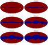 |
Fig. 4 Six masks with Fsky ∈ { 0.98,0.93,0.87,0.77,0.67,0.57 }. The masked area is in blue. |
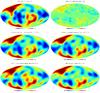 |
Fig. 5 Top: input-smoothed simulated CMB map (ℓmax = 10) and the same map, but masked (Fsky = 77%) and not smoothed (i.e., input-simulated data). Middle: inpainting of the top right image up to ℓmax = 10, using a sparsity prior (left) and an energy prior (right). Bottom: inpainting of the top right image up to ℓmax = 10, using an isotropy prior (left) and a simple Fsky correction (right). |
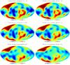 |
Fig. 6 ℓ1 sparsity-based inpainting of a simulated CMB map with different masks. Top: Fsky = 98% and 93%, middle: 87% and 77%, and bottom: 67% and 57%. |
We now turn to the projection on .
We begin by noting that this set is separable, i.e.,
 ,
,
where Bℓ is the band depicted Fig. 2. It turns out that for fixed μ,
Bℓ is so-called prox-regular since its associated
orthogonal projector is single-valued with a closed-form. Indeed, the projector onto
 is
is  (4)where
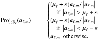 (5)
(5)
Choice of the constraint radius:
to devise a meaningful choice (from a statistical perspective) of the constraint
radius ε, we first need to derive the null distribution1 of
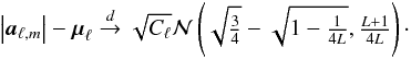
|aℓ,m| − μℓ,∀(ℓ,m),
with the particular case when  .
aℓ,m being the spherical
harmonic coefficients of a zero-mean stationary and isotropic Gaussian process whose
angular power spectrum is Cℓ, it is easy to
show that
.
aℓ,m being the spherical
harmonic coefficients of a zero-mean stationary and isotropic Gaussian process whose
angular power spectrum is Cℓ, it is easy to
show that 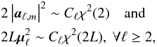 where
L = 2ℓ + 1. By the Fisher asymptotic formula, we
then obtain
where
L = 2ℓ + 1. By the Fisher asymptotic formula, we
then obtain 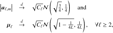 where
where
 means convergence
in distribution. Thus, ignoring the obvious dependency between
|aℓ,m| and
μℓ, we obtain
means convergence
in distribution. Thus, ignoring the obvious dependency between
|aℓ,m| and
μℓ, we obtain
 The
distribution of this difference can be derived properly using the delta method in law,
but computing the covariance matrix of the augmented vector
(aℓ,m)m,
remains a problem. The quality of the above asymptotic approximation increases as
ℓ increases.
The
distribution of this difference can be derived properly using the delta method in law,
but computing the covariance matrix of the augmented vector
(aℓ,m)m,
remains a problem. The quality of the above asymptotic approximation increases as
ℓ increases.
The upper and lower critical thresholds at the double-sided significance level
0 ≤ α ≤ 1 are 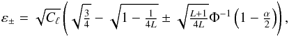 where
Φ is the standard normal cumulative distribution function.
where
Φ is the standard normal cumulative distribution function.
We depict in Fig. 3 the upper and lower critical
thresholds normalized by  at the classical significance level 0.05 as a function of ℓ. One can
observe that the thresholds are not symmetric. This entails that different values of
ε should be used in Eq. (5). Furthermore, as expected, the two thresholds decrease in magnitude as
ℓ increases. They attain a plateau for ℓ that is
sufficiently high (typically ≥ 100). It is easy to see that the two limit values are
at the classical significance level 0.05 as a function of ℓ. One can
observe that the thresholds are not symmetric. This entails that different values of
ε should be used in Eq. (5). Furthermore, as expected, the two thresholds decrease in magnitude as
ℓ increases. They attain a plateau for ℓ that is
sufficiently high (typically ≥ 100). It is easy to see that the two limit values are
 and
and
 .
.
The isotropy-constrained inpainting algorithm is given is Appendix D.
6. Experiments
6.1. aℓ,m reconstruction
In this section, we compare the different inpainting methods described above: the
DR-sparsity prior inpainting, the DR-energy prior inpainting, and the isotropy prior
inpainting. We also test the case of no-inpainting by applying just an Fsky correction to
the aℓ,m spherical harmonic
coefficients of the map (i.e., data aℓ,m are
corrected with a correction term equal to  ). We
ran 100 CMB Monte-Carlo simulations with a resolution corresponding to nside equal to 32,
which is precise enough for the large scales we are considering. We considered six
different masks with sky coverage Fsky of
{ 0.98,0.93,0.87,0.77,0.67,0.57 }.
). We
ran 100 CMB Monte-Carlo simulations with a resolution corresponding to nside equal to 32,
which is precise enough for the large scales we are considering. We considered six
different masks with sky coverage Fsky of
{ 0.98,0.93,0.87,0.77,0.67,0.57 }.
Figure 4 displays these masks. Point source masks were not considered here, since they should not affect aℓ,m estimation at very low multipole. Each of these simulated CMB maps was masked with the six masks. Figure 5 top right shows one CMB realization masked with the 77% Fsky mask. Figure 5 middle and bottom show the inpainting of the Fig. 5 top right image with the four methods (i.e., using sparsity, energy, isotropy priors, and Fsky correction). Figure 6 depicts the results given by the ℓ1 sparsity-based inpainting method for the six different masks. We can clearly see that the quality of the reconstruction degrades with decreasing sky coverage.
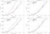 |
Fig. 7 Relative MSE (in percent) per ℓ versus sky coverage for different multipoles. See text for details. |
The aℓ,m coefficients of the six hundred maps (100 realizations masked with the six different masks) were then estimated using the three inpainting methods and the Fsky correction methods. The approaches were compared in terms of the relative MSE and relative MSE per ℓ; see end of Sect. 3 for their definition.
Figure 7 shows the relative MSE for ℓ = 2 to 5 versus the sky coverage Fsky. The three horizontal lines correspond to 1%, 5%, and 10% of the cosmic variance (CV). Inpainting based on the sparsity and energy priors give relatively close results, which are better than the one assuming the isotropy prior or the Fsky correction. It is interesting to notice that a very high quality reconstruction (with 1% of the CV) can be obtained with both the sparsity- and energy-based inpainting methods up to ℓ = 4 for a mask with an Fsky exceeding 80%. If WMAP data do not allow us to study non-Gaussianity with such a small mask, Planck component separation will certainly be able to achieve the required quality to enable make possible the useusing of such a small Galactic mask. With a 77%-coverage Galactic mask, the error increases by a factor 5 at ℓ = 4 !
Figure 8 shows the same errors, but they are now plotted versus the multipoles for the six different masks. The ℓ1 sparsity-based inpainting method seems to be slightly better than the one based on the energy prior, especially when the sky coverage decreases.
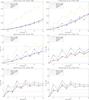 |
Fig. 8 Relative MSE in percent per sky coverage versus ℓ for the six masks. |
6.2. Anomalies in CMB maps
One of the main motivations of recovering full-sky maps is to be able to study
statistical properties such as Gaussianity and statistical isotropy on large scales.
Statistical isotropy is violated if there exists a preferred axis in the map. Mirror
parity, i.e., parity with respect to reflections through a plane:
 , where
 is the normal vector to the plane, is an example of a statistic where a preferred axis can
be sought (Ben-David et al. 2012; Land & Magueijo 2005).
is the normal vector to the plane, is an example of a statistic where a preferred axis can
be sought (Ben-David et al. 2012; Land & Magueijo 2005).
With full-sky data, one can estimate the S-map for a given multipole in
spherical harmonics by considering (Ben-David et al.
2012): 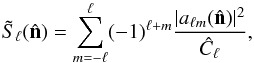 (6)where
 corresponds to the value of the aℓm
coefficients when the map is rotated to have
as the z-axis. Positive (negative) values of
corresponds to the value of the aℓm
coefficients when the map is rotated to have
as the z-axis. Positive (negative) values of
 correspond to even (odd)
mirror parities in the
direction. The same statistic can also be considered summed over all low multipoles one
wishes to consider(e.g., focusing only on low multipoles as in Ben-David et al. 2012):
correspond to even (odd)
mirror parities in the
direction. The same statistic can also be considered summed over all low multipoles one
wishes to consider(e.g., focusing only on low multipoles as in Ben-David et al. 2012):
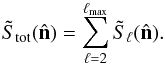 (7)It is convenient
to redefine the parity estimator as
(7)It is convenient
to redefine the parity estimator as  , so
that ⟨S⟩ = 0.
, so
that ⟨S⟩ = 0.
The most even and odd mirror-parity directions for a given map can be considered by
estimating (Ben-David et al. 2012)
 (8)
(8) (9)where
μ(S) and σ(S) are
the mean and standard deviation of the S map. The quantities
S+ and S− each correspond to
different axes
(9)where
μ(S) and σ(S) are
the mean and standard deviation of the S map. The quantities
S+ and S− each correspond to
different axes  and
and
 and are the quantities
which we consider when discussing mirror parity in CMB maps.
and are the quantities
which we consider when discussing mirror parity in CMB maps.
To use inpainted maps to study mirror parity, it is crucial that the inpainting method constitutes a bias-free reconstruction method, i.e., that it does not destroy existing mirror parities nor that it creates previously inexistent mirror parity anomalies.
In order to test this, we considered three sets of 1000 simulated CMB maps using a WMAP7 best-fit cosmology with nside = 32, one set for each inpainting prior. For each simulation we calculated the mirror parity estimators S±. We isolated the anomalous maps, defined as those whose S± value is higher than twice the standard deviation given by the simulations. This yielded 34 maps (3.4%) for the even mirror parity and 40 maps (4%) for the odd mirror parity in the full-sky simulations.
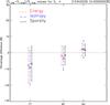 |
Fig. 9 Percentage difference between anomalous (i.e., high) odd mirror parity scores (S−) before (i.e., full-sky) and after inpainting for three different inpainting priors. |
Since recent work showed a potential odd-mirror anomaly in WMAP data (Ben-David et al. 2012), we focused on testing for potential biases in odd-mirror anomalies. Figure 9 shows the percentage difference between the true S− value and the one estimated from the inpainted map. For this statistical test, the result does not depend on the inpainting method because the three different priors give similar biases and error bars. For positive-mirror anomalies, we find similar results (not shown in figure). Similarly to the previous experiment, we can see that a very good estimation of the parity statistic can be achieved for masks with Fsky exceeding 0.8.
7. Software and reproducible research
To support reproducible research, the developed IDL code will be released with the next version of ISAP (Interactive Sparse astronomical data Analysis Packages) via the web site: http://www.cosmostat.org
All experiments were performed using the default options
-
Sparsity:
Alm = cmb_lowl_alm_inpainting(CMBMap, Mask, /sparsity)
-
Energy:
Pd = mrs_powspec( CMBMap, Mask)
P = mrs_deconv_powspec( pd, Mask)
Alm = cmb_lowl_alm_inpainting(CMBMap, /Energy, Prea=P)
-
Isotropy:
Pd = mrs_powspec( CMBMap, Mask)
P = mrs_deconv_powspec( Pd, Mask)
Alm = cmb_lowl_alm_inpainting(CMBMap, /Isotropy, Prea=P)
8. Conclusion
We have investigated three priors to regularize the CMB inpainting problem: Gaussianity, sparsity, and isotropy. To solve the corresponding minimization problems, we also proposed fast novel algorithms, based for instance on proximal splitting methods for convex non-smooth optimization. We found that both Gaussianity and ℓ1 sparsity priors lead to very good results. The isotropy prior does not provide comparably good results. The sparsity prior seems to lead to slightly better results for ℓ > 2, and more robust when the sky coverage decreases. Furthermore, unlike the energy-prior based inpainting, the sparsity-based one does not require a power spectrum as an input, which is a significant advantage.
Then we evaluated the reconstruction quality as a function of the sky coverage and saw that a high-quality reconstruction, within 1% of the cosmic variance, can be reached for a mask with an Fsky exceeding 80%. We also studied mirror-parity anomalies and found that mask with an Fsky exceeding 80% also permitted nearly bias-free reconstructions of the mirror parity scores. Such a mask seems unrealistic for a WMAP data analysis, but it could and should be a target for Planck component separation methods. To know if this 80% mask is realistic for Planck, we will need more realistic simulations including the ISW effect, and residual foregrounds at amplitudes similar to those achieved by the actual best Planck component separation methods. Another interesting study will consist of comparing the sparse inpainting to other methods such as the maximum likelihood or the Wiener filtering (Ben-David et al. 2012; Feeney et al. 2011).
Appendix A: Algorithm for the l 0 problem
Solving Eq. (2)when q = 0
is known to be NP-hard. This is further complicated by the presence of the non-smooth
constraint term. Iterative Hard thresholding (IHT) attempts to solve this problem through
the following scheme  (10)where the nonlinear
operator
(10)where the nonlinear
operator  is a
term-by-term hard thresholding, i.e.
is a
term-by-term hard thresholding, i.e.  , where
 if
| ai| > λ
and 0 otherwise. The threshold parameter λn
decreases with the iteration number and is supposed to play a role similar to the cooling
parameter in simulated annealing, i.e. hopefully it allows to avoid stationary points and
local minima.
if
| ai| > λ
and 0 otherwise. The threshold parameter λn
decreases with the iteration number and is supposed to play a role similar to the cooling
parameter in simulated annealing, i.e. hopefully it allows to avoid stationary points and
local minima.
Appendix B: Algorithm for the l 1 problem
It is now well-known that l1 norm is the tightest convex relaxation (in the ℓ2 ball) of the l0 penalty (Starck et al. 2010). This suggests solving Eq. (2)with q = 1. In this case, the problem is well-posed: it has at least a minimizer, and all minimizers are global. Furthermore, although it is completely non-smooth, it can be solved efficiently with a provably convergent algorithm that belongs to the family of proximal splitting schemes (Combettes & Pesquet 2011; Starck et al. 2010).
In particular, we propose to use the Douglas-Rachford (DR) splitting scheme. Let
β > 0,  be a sequence in ]0, 2[ such that
∑ t ∈Nαn(2 − αn) = +∞.
The DR recursion, applied to Eq. (2)with
q = 1, reads
be a sequence in ]0, 2[ such that
∑ t ∈Nαn(2 − αn) = +∞.
The DR recursion, applied to Eq. (2)with
q = 1, reads 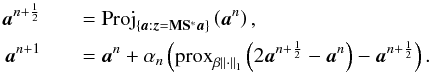 (11)proxβ∥·∥1is
the proximity operator of the l1-norm, which can be easily shown
to be soft-thresholding
(11)proxβ∥·∥1is
the proximity operator of the l1-norm, which can be easily shown
to be soft-thresholding 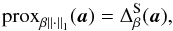 (12)where
 and
and
 .
Proj{ a:z = MS∗a }
is the orthogonal projector on the corresponding set, and it consists of taking the inverse
spherical harmonic transform of its argument, setting its pixel values to the observed ones
at the corresponding locations, and taking the forward spherical harmonic transform. It can
be shown that the sequence
.
Proj{ a:z = MS∗a }
is the orthogonal projector on the corresponding set, and it consists of taking the inverse
spherical harmonic transform of its argument, setting its pixel values to the observed ones
at the corresponding locations, and taking the forward spherical harmonic transform. It can
be shown that the sequence  converges to a global minimizer of Eq. (2)for
q = 1.
converges to a global minimizer of Eq. (2)for
q = 1.
Appendix C: Algorithm for the l 2 problem,
This scheme is based again on Douglas-Rachford splitting applied to solve problem Eq.
(3). Its steps are  (13)where
β and αn are defined as
above, and the proximity operator of the squared weighted
ℓ2-norm is
(13)where
β and αn are defined as
above, and the proximity operator of the squared weighted
ℓ2-norm is  (14)where ⊗ stands for the
entry-wise multiplication between two vectors, and the division is also to be understood
entry-wise. The projector
Proj{x:z = Mx}
has a simple closed-form and consists in setting pixel values to the observed ones at the
corresponding
(14)where ⊗ stands for the
entry-wise multiplication between two vectors, and the division is also to be understood
entry-wise. The projector
Proj{x:z = Mx}
has a simple closed-form and consists in setting pixel values to the observed ones at the
corresponding
locations, and keeping the others intact. It can be shown that the sequence
 converges to the unique global minimizer of Eq. (3).
Appendix D: Algorithm for isotropy inpainting
The isotropy-constrained inpainting problem can be cast as the non-convex
feasibility problem  (15)The feasible set is
nonempty since the constraint set is non-empty and closed; the CMB is in it under the
isotropy hypothesis. To solve Eq. (15), we
propose to use the von Neumann method of alternating projections onto the two constraint
sets, whose recursion can be written
(15)The feasible set is
nonempty since the constraint set is non-empty and closed; the CMB is in it under the
isotropy hypothesis. To solve Eq. (15), we
propose to use the von Neumann method of alternating projections onto the two constraint
sets, whose recursion can be written
 (16)Using closedness and
prox-regularity of the constraints, and by arguments from Lewis & Malick (2008), we can conclude that our non-convex alternating
projections algorithm for inpainting converges locally to a point of the intersection
(16)Using closedness and
prox-regularity of the constraints, and by arguments from Lewis & Malick (2008), we can conclude that our non-convex alternating
projections algorithm for inpainting converges locally to a point of the intersection
 which is non-empty.
That is the distribution under the isotropy hypothesis.
Acknowledgments
The authors would like to thank Hiranya Peiris and Stephen Feeney for useful discussions. This work was supported by the French National Agency for Research (ANR -08-EMER-009-01), the European Research Council grant SparseAstro (ERC-228261), and the Swiss National Science Foundation (SNSF).
References
- Abrial, P., Moudden, Y., Starck, J., et al. 2007, J. Fourier Anal. Appl., 13, 729 [Google Scholar]
- Abrial, P., Moudden, Y., Starck, J., et al. 2008, Stat. Meth., 5, 289 [NASA ADS] [CrossRef] [Google Scholar]
- Ben-David, A., Kovetz, E. D., & Itzhaki, N. 2012, ApJ, 748, 39 [NASA ADS] [CrossRef] [Google Scholar]
- Bobin, J., Starck, J.-L., Sureau, F., & Basak, S. 2012, A&A, in press DOI: 10.1051/0004-6361/201219781 [Google Scholar]
- Bucher, M., & Louis, T. 2012, MNRAS, 3271 [Google Scholar]
- Combettes, P. L., & Pesquet, J.-C. 2011, Fixed-Point Algorithms for Inverse Problems in Science and Engineering (Springer-Verlag), 185 [Google Scholar]
- de Oliveira-Costa, A., & Tegmark, M. 2006, Phys. Rev. D, 74, 023005 [NASA ADS] [CrossRef] [Google Scholar]
- Dupé, F.-X., Rassat, A., Starck, J.-L., & Fadili, M. J. 2011, A&A, 534, A51 [NASA ADS] [CrossRef] [EDP Sciences] [Google Scholar]
- Feeney, S. M., Peiris, H. V., & Pontzen, A. 2011, Phys. Rev. D, 84, 103002 [NASA ADS] [CrossRef] [Google Scholar]
- Hivon, E., Górski, K. M., Netterfield, C. B., et al. 2002, ApJ, 567, 2 [NASA ADS] [CrossRef] [Google Scholar]
- Kim, J., Naselsky, P., & Mandolesi, N. 2012, ApJ, 750, L9 [NASA ADS] [CrossRef] [Google Scholar]
- Land, K., & Magueijo, J. 2005, Phys. Rev. Lett., 72, 101302 [Google Scholar]
- Lewis, A., & Malick, J. 2008, Math. Oper. Res., 33, 216 [NASA ADS] [CrossRef] [Google Scholar]
- Paykari, P., Starck, J.-L., & Fadili, M. J. 2012, A&A, 541, A74 [NASA ADS] [CrossRef] [EDP Sciences] [Google Scholar]
- Perotto, L., Bobin, J., Plaszczynski, S., Starck, J., & Lavabre, A. 2010, A&A, 519, A4 [NASA ADS] [CrossRef] [EDP Sciences] [Google Scholar]
- Pires, S., Starck, J., Amara, A., et al. 2009, MNRAS, 395, 1265 [NASA ADS] [CrossRef] [Google Scholar]
- Pires, S., Starck, J., & Refregier, A. 2010, IEEE Sign. Proc. Mag., 27, 76 [NASA ADS] [CrossRef] [Google Scholar]
- Plaszczynski, S., Lavabre, A., Perotto, L., & Starck, J.-L. 2012, A&A, 544, A27 [NASA ADS] [CrossRef] [EDP Sciences] [Google Scholar]
- Rassat, A., Starck, J.-L., & Dupe, F. X. 2012, A&A, submitted [Google Scholar]
- Sato, K. H., Garcia, R. A., Pires, S., et al. 2010, Astron. Nachr., submitted [arXiv:1003.5178] [Google Scholar]
- Schmitt, J., Starck, J. L., Casandjian, J. M., Fadili, J., & Grenier, I. 2010, A&A, 517, A26 [NASA ADS] [CrossRef] [EDP Sciences] [Google Scholar]
- Starck, J.-L., Murtagh, F., & Fadili, M. 2010, Sparse Image and Signal Processing (Cambridge University Press) [Google Scholar]
- Zacchei, A., Maino, D., Baccigalupi, C., et al. 2011, A&A, 536, A5 [NASA ADS] [CrossRef] [EDP Sciences] [Google Scholar]
All Figures
|
Fig. 1 Relative MSE per ℓ in percent for the two sparsity-based inpainting algorithms, IHT (dashed red line) and DR (continuous black line). |
| In the text | |
|
Fig. 2 Set Bℓ. |
| In the text | |
|
Fig. 3 Normalized critical thresholds at the significance level 0.05 as a function of ℓ. |
| In the text | |
|
Fig. 4 Six masks with Fsky ∈ { 0.98,0.93,0.87,0.77,0.67,0.57 }. The masked area is in blue. |
| In the text | |
|
Fig. 5 Top: input-smoothed simulated CMB map (ℓmax = 10) and the same map, but masked (Fsky = 77%) and not smoothed (i.e., input-simulated data). Middle: inpainting of the top right image up to ℓmax = 10, using a sparsity prior (left) and an energy prior (right). Bottom: inpainting of the top right image up to ℓmax = 10, using an isotropy prior (left) and a simple Fsky correction (right). |
| In the text | |
|
Fig. 6 ℓ1 sparsity-based inpainting of a simulated CMB map with different masks. Top: Fsky = 98% and 93%, middle: 87% and 77%, and bottom: 67% and 57%. |
| In the text | |
|
Fig. 7 Relative MSE (in percent) per ℓ versus sky coverage for different multipoles. See text for details. |
| In the text | |
|
Fig. 8 Relative MSE in percent per sky coverage versus ℓ for the six masks. |
| In the text | |
|
Fig. 9 Percentage difference between anomalous (i.e., high) odd mirror parity scores (S−) before (i.e., full-sky) and after inpainting for three different inpainting priors. |
| In the text | |
Current usage metrics show cumulative count of Article Views (full-text article views including HTML views, PDF and ePub downloads, according to the available data) and Abstracts Views on Vision4Press platform.
Data correspond to usage on the plateform after 2015. The current usage metrics is available 48-96 hours after online publication and is updated daily on week days.
Initial download of the metrics may take a while.