| Issue |
A&A
Volume 550, February 2013
|
|
|---|---|---|
| Article Number | A32 | |
| Number of page(s) | 7 | |
| Section | Stellar structure and evolution | |
| DOI | https://doi.org/10.1051/0004-6361/201117913 | |
| Published online | 21 January 2013 | |
Constraining magnetic-activity modulations in three solar-like stars observed by CoRoT and NARVAL
1 High Altitude Observatory, NCAR, PO Box 3000, Boulder, CO 80307, USA
e-mail: This email address is being protected from spambots. You need JavaScript enabled to view it.
2 Laboratoire AIM, CEA/DSM-CNRS-Université Paris Diderot; IRFU/SAp, Centre de Saclay, 91191 Gif-sur-Yvette Cedex, France
e-mail: This email address is being protected from spambots. You need JavaScript enabled to view it.
3 CNRS, Institut de Recherche en Astrophysique et Planétologie, 14 avenue Edouard Belin, 31400 Toulouse, France
e-mail: This email address is being protected from spambots. You need JavaScript enabled to view it.
; This email address is being protected from spambots. You need JavaScript enabled to view it.
; This email address is being protected from spambots. You need JavaScript enabled to view it.
;
4 Université de Toulouse, UPS-OMP, IRAP, 31400 Toulouse, France
5 Laboratoire Lagrange, UMR7293, Université de Nice Sophia-Antipolis, CNRS, Observatoire de la Côte d’Azur, BP 4229, 06304 Nice Cedex 4, France
e-mail: This email address is being protected from spambots. You need JavaScript enabled to view it.
6 Instituto de Astrofísica de Canarias, 38200 La Laguna, Tenerife, Spain
e-mail: This email address is being protected from spambots. You need JavaScript enabled to view it.
7 Departamento de Astrofísica, Universidad de La Laguna, 38206 La Laguna, Tenerife, Spain
8 LESIA, CNRS, Université Pierre et Marie Curie, Université Denis Diderot, Observatoire de Paris, 92195 Meudon Cedex, France
e-mail: This email address is being protected from spambots. You need JavaScript enabled to view it.
Received: 18 August 2011
Accepted: 28 November 2011
Abstract
Context. Stellar activity cycles are the manifestation of dynamo process running in the stellar interiors. They have been observed from years to decades thanks to the measurement of stellar magnetic proxies on the surface of the stars, such as the chromospheric and X-ray emissions, and to the measurement of the magnetic field with spectropolarimetry. However, all of these measurements rely on external features that cannot be visible during, for example, a Maunder-type minimum. With the advent of long observations provided by space asteroseismic missions, it has been possible to penetrate the stars and study their properties. Moreover, the acoustic-mode properties are also perturbed by the presence of these dynamos.
Aims. We track the temporal variations of the amplitudes and frequencies of acoustic modes allowing us to search for signature of magnetic activity cycles, as has already been done in the Sun and in the CoRoT target HD 49933.
Methods. We used asteroseimic tools and more classical spectroscopic measurements performed with the NARVAL spectropolarimeter to check that there are hints of any activity cycle in three solar-like stars observed continuously for more than 117 days by the CoRoT satellite: HD 49385, HD 181420, and HD 52265. To consider that we have found a hint of magnetic activity in a star we require finding a change in the amplitude of the p modes that should be anti-correlated with a change in their frequency shifts, as well as a change in the spectroscopic observations in the same direction as the asteroseismic data.
Results. Our analysis gives very small variation in the seismic parameters preventing us from detecting any magnetic modulation. However, we are able to provide a lower limit of any magnetic-activity change in the three stars that should be longer than 120 days, which is the length of the time series. Moreover we computed the upper limit for the line-of-sight magnetic field component being 1, 3, and 0.6 G for HD 49385, HD 181420, and HD 52265, respectively. More seismic and spectroscopic data would be required to have a firm detection in these stars.
Key words: asteroseismology / methods: data analysis / stars: solar-type / stars: activity / stars: general
© ESO, 2013
1. Introduction
The physical processes behind the dynamos producing magnetic activity cycles in stars have not yet been explained perfectly (e.g., Browning et al. 2006; Lanza 2010, and references there in). Observing many stars showing magnetic cycles could help for better understanding their dependence with the stellar properties and the place occupied by the Sun in this context. Moreover, the features on the surface of the stars, in particular their magnetism, are extremely important for understanding the characteristics of stellar neighbourhoods and, therefore, the properties and conditions in the exoplanets systems (e.g., Ribas et al. 2010, and references therein).
Stellar activity cycles have been measured for a long time (e.g., Wilson 1978; Baliunas & Vaughan 1985; Baliunas et al. 1995; Hall et al. 2007) mostly thanks to variations related to the presence of starspots crossing the visible stellar disk (e.g., Strassmeier 2009). Indeed, in many cases, these cycles were in a range of 2.5 to 25 years. Based on emission proxies, Batalha et al. (2002) could estimate that about two-thirds of the solar-type stars lie in the same range of magnetism as the Sun (minimum to maximum) with one-third of them being more magnetically active. Recently, spectropolarimetric observations of cool active stars unveiled the evolution of magnetic topologies of cool stars across their magnetic cycles, witnessed as polarity reversals of their large-scale surface field (Fares et al. 2009; Petit et al. 2009). More recently, other short activity cycles have also been detected using chromospheric activity indexes (Metcalfe et al. 2010). With all this information, it has been suggested that the length of the activity cycle increases proportionally to the stellar rotational periods along two distinct paths in main-sequence stars: the active and the inactive stars (Saar & Brandenburg 1999; Böhm-Vitense 2007).
Most of the activity-cycle studies are based, however, on proxies of the surface magnetism at different wavelengths. This could be a problem because solar-like stars can suffer from periods of extended minima as happened to the Sun during the Maunder minimum or between cycles 23 and 24. Nevertheless, during this unexpectedly long minimum, there was seismic evidence for the start of a new cycle in 2008 whereas the classical surface indicators were still at a low level (Salabert et al. 2009; Fletcher et al. 2010).Besides this, Beer et al. (1998) have shown that during the Maunder minimum while no sunspots were visible on the surface, internal changes seemed to be going on. Therefore, having complementary diagnostics on the internal magnetic activity of the stars could help better understand the coupling between internal and external manifestations of magnetic phenomena.
It is now well known that the frequencies of the solar acoustic (p) modes change with the solar activity level (see Woodard & Noyes 1985; Pallé et al. 1989). These changes in p modes are induced by the perturbations of the solar structure in the photosphere and just below it (e.g., Goldreich et al. 1991; Chaplin et al. 2001). Therefore, the variation in the mean values of several global p-mode properties with the magnetic cycle – with different geometrical weights – will be sensitive to overall changes in the structure of the Sun and not to a particular spot crossing the visible solar disk.
The advent of long and continuous asteroseismic measurements, provided by the recent spacecrafts, such as CoRoT (Convection Rotation and planetary Transits, Baglin et al. 2006; Michel et al. 2008) or Kepler (Borucki et al. 2010; Chaplin et al. 2011b, for a description of the solar-like observations done with this instrument), allows us to study magnetic activity cycles by means of p-mode frequencies and amplitudes, as has already been done for the Sun using Sun-as-a-star observations (e.g., Anguera Gubau et al. 1992; Jiménez-Reyes et al. 2004). This technique has already been used successfully on HD 49933, a solar-like star observed by CoRoT (García et al. 2010; Salabert et al. 2011b). These same observations can also be used to study the surface magnetism with starspot proxies (García et al. 2010; Chaplin et al. 2011a) or with spot-modelling techniques (e.g., Mosser et al. 2009; Mathur et al. 2010a).
In this work, we study the temporal variations in the p-mode characteristics of three of the highest signal-to-noise ratio solar-like stars observed by CoRoT during more than 117 continuous days: HD 49385 (Deheuvels et al. 2010), HD 181420 (Barban et al. 2009), and HD 52265 (Ballot et al. 2011). In Sect. 2 we describe the methodology followed in this paper to analyse both the asteroseismic and spectroscopic observations. Then, in Sect. 3, we discuss the results obtained for each of the three stars studied. Finally, we give our conclusions in Sect. 4.
Frequency range used to compute the averaged frequency shift and Amax of the 3 stars.
2. Methodology and data analysis
2.1. Asteroseismic parameters
Acoustic-mode parameters were obtained from the analysis of subseries of 30 days, shifted every 15 days, therefore, only every other point is independent. We chose this length of subseries to have a good trade-off between having good enough resolution in the acoustic modes and enough subseries to study a hypothetical cycle. We had checked with solar observations (using the Global Oscillation at Low Frequency (Gabriel et al. 1995; García et al. 2005) instrument aboard the Solar Heliospheric Observatory) that the differences between different lengths of subseries are well within the uncertainties. In each of the subseries we used, individual p-mode frequencies were extracted with a maximum likelihood estimator (Anderson et al. 1990). We fitted Lorentzian profiles with a local approach on successive series of l = 0, 1, and 2 modes (Salabert et al. 2004).
The background was fitted using a Harvey-like profile describing the granulation (e.g., Harvey 1985; Mathur et al. 2011b). The amplitude ratio between the l = 0, 1, and 2 modes was fixed to 1, 1.5, and 0.5 respectively (Salabert et al. 2011a), and only one linewidth was fitted per radial order. For HD 52265, the rotational splitting and the inclination angle of the star were fixed to the values given in Ballot et al. (2011). For the other two stars, HD 181420 and HD 49385, because of less reliable estimates in these parameters, no splitting and no inclination angle were fitted, i.e. only one Lorentzian profile was used to model each of the modes as is commonly done in cases where the linewidth of the modes is too big to properly disentangle the splitting or else when the signal-to-noise ratio is low (e.g., Mathur et al. 2011a). The mode identification #1 from Barban et al. (2009) and from Deheuvels et al. (2010) were respectively used. Table 1 summarizes the frequency range used to compute the averaged frequency shift of each star. It is important to note that we also used cross-correlation techniques (Pallé et al. 1989; García et al. 2010) to compute the frequency shifts in a global way. The results of both methods are quantitatively the same within their uncertainties. For the sake of clarity we therefore decided to show the frequency shifts obtained by the first method alone.
To extract the maximum amplitude per radial mode, Amax, we used the method described by Mathur et al. (2010b), fully tested with the Kepler targets (Huber et al. 2010; Hekker et al. 2011; Verner et al. 2011; Mosser et al. 2012). Briefly, we first subtract the background model (one Harvey-law function as explained previously) fitted including a white noise component from the power density spectrum (PDS). We then smooth the PDS over 3 × ⟨ Δν ⟩ , where ⟨ Δν ⟩ is the mean large separation obtained with the A2Z pipeline (Mathur et al. 2010b). Finally, we fit a Gaussian function around the p-mode bump giving us the maximum height of the modes. This power, Pmax, is converted into a bolometric amplitude, Amax, by using the method based on Kjeldsen et al. (2008) and adapted to CoRoT by Michel et al. (2009), following the formula, 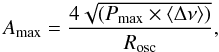 (1)where the response function Rosc for CoRoT observations given by Michel et al. (2009) is
 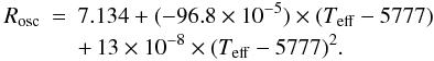 (2)The frequency interval used in this analysis is defined in the last column of Table 1. We used different frequency ranges when we computed the frequency shifts and when we computed the maximum amplitude of the modes. Indeed, for measuring the frequency shift, we fitted individual modes. We needed a high signal-to-noise ratio to have lower uncertainties in the frequency shifts leading to a very narrow frequency range. To measure the maximum amplitude per radial mode, we fit a Gaussian function over the p-mode bump and thus, generally, we needed a much broader frequency range.
For each star we also calculated a starspot proxy, as described in García et al. (2010) and Chaplin et al. (2011a), i.e., we computed the standard deviation of the light curve of each subseries, which gives some information on the fluctuation of the brightness of the star. We assumed that this modulation is due to starspots crossing the visible stellar disk. Indeed, the photometry of these CoRoT targets is dominated by the stellar signal and not by the photon noise. Taking as an example HD 52265, the measured level of the photon noise is ~ 0.5 ppm2/μHz (Ballot et al. 2011), i.e. ~ 88 ppm in the flux, which is three to four times less than the dispersion we had measured with the magnetic proxy. However, the starspot proxy could be more perturbed than the global p modes. If a large spot crosses the visible stellar disk, on the one hand, it will induce a more or less significant fluctuation in the light curve hence in the starspot proxy. On the other hand, the global p modes will not be affected because they are sensitive to the global magnetic field of the star. As a consequence, there could be a mismatch between the evolution of the starspot proxy and the p modes.
To follow the time evolution of structures in the frequency domain all along the length of the observations, we analysed the time series with the wavelet tool (Torrence & Compo 1998; Liu et al. 2007). In our case, we took the Morlet wavelet, which is the product of a sinusoid and a Gaussian function and we calculated the wavelet power spectrum (WPS). By collapsing the WPS along the time axis, we obtained the global wavelet power spectrum (GWPS). With this technique, we were able to track the temporal evolution of the starspots and look for any increase in the activity level while we could verify the presence of any harmonic of the rotation at lower frequency. Indeed, the wavelet analysis reconstructs the signal by putting most of the power in the fundamental harmonic reducing the leakage on the overtones. An example of the use of this technique of studying the solar activity cycle and the rotation period of the Sun during the last three cycles (using a combination of real data and simulations) can be seen in Vázquez Ramió et al. (2011). In that analysis it is shown how the main signature in the WPS is the rotation period at ~ 26 days instead of the first overtone at ~ 13 days, which is the most important peak in the power spectrum of the Sun at low frequency for photometric and Doppler velocity observations (except during the minimum activity periods where no signal of the rotation can be measured above the general background level). We computed the 95% confidence level for the GWPS to quantify the detection of a peak. The 95% confidence levels were obtained as described in Sect. 5 of Torrence & Compo (1998) knowing that the GWPS has a χ2 distribution.
2.2. Spectroscopic analyses
To complement the seismic studies, we observed our sample of three stars with the NARVAL spectropolarimeter placed at the Bernard Lyot, a 2 m telescope at the Pic du Midi Observatory (Aurière 2003). The instrumental setup (in its polarimetric mode) and reduction pipeline are strictly identical to the one described by Petit et al. (2008). With the adopted instrumental configuration, it was possible to perform the simultaneous recording of a high-resolution spectrum in unpolarised and circularly polarised light. Except for a fraction of the data sets collected for HD 52265 and HD 181420, the available spectroscopic material is not contemporaneous to the CoRoT runs.
We used the unpolarised spectrum to estimate the stellar chromospheric emission in the cores of the Ca ii H spectral line. We employed the same approach as the one used by Wright et al. (2004) to calculate an activity proxy calibrated against Mount Wilson S-index measurements.
For the Sun, the variations in the S index are ~0.04, while the associated uncertainties in stellar measurements are typically 10-3. Therefore the uncertainties are one order of magnitude smaller than the S-index variations for a star like the Sun. This sensitivity is enough to detect a stellar cycle that is similar to the one observed in the Sun.
In a highly sensitive search for Zeeman signatures generated by a large-scale photospheric field, we extracted from each polarised spectrum a mean photospheric line profile with enhanced signal-to-noise ratio, using the cross-correlation method as defined by Donati et al. (1997). The line-of-sight component of the magnetic field was then calculated with the centre-of-gravity technique (Rees & Semel 1979).
3. Results
3.1. HD 49385
HD 49385 is a G-type star that is more evolved than the Sun, so it is placed in the HR diagram at the end of the main sequence or lying shortly after it. The effective temperature, Teff, is about 6095 ± 65 K, and it has a projected rotational velocity of  km s-1. The seismic analysis of the CoRoT data provides a mean large spacing, ⟨ Δν ⟩ = 56.3 μHz, and the frequency of the maximum amplitude of the p-mode bump, νmax, of 1013 μHz (see a detailed compilation of the parameters of the star in Deheuvels et al. 2010).
Unfortunately, for this star the analysis of the light curve does not provide with certainty the surface rotation period, any more than the rotational splittings of the acoustic modes do not provide the internal rotation. Deheuvels et al. (2010) explain that there might be a hint of the rotation period, Prot, at around ten days. However, the WPS shown in Fig. 1, does present some enhanced power around 29 days as well, with much higher power than the peak at about ten days. Unfortunately, the cone of influence, which shows the region where the WPS is reliable, is too close to this value, so longer observations would be needed to confirm such periodicity. We note that this longer rotation period is compatible with the spectroscopic vsini when we use the seismic parameters combined with the effective temperature given above and a radius of R = 1.96 R⊙ obtained from the scaling relations based on solar values (Kjeldsen & Bedding 1995; Huber et al. 2011). Indeed, with this longer rotation rate, a wider range of stellar-inclination angles (60 ± 30°) are allowed than if the rotation of ten days is considered. A period of 29 days also agrees with the Skumanich law (Skumanich 1972), which gives ~27 days when assuming an age of 5 Gyr as given from the model of Deheuvels & Michel (2011), as well as with the Asteroseismic Modeling Portal (Metcalfe et al. 2009; Mathur et al. 2012).
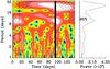 |
Fig. 1 Left panel: wavelet power spectrum (WPS) as a function of time of HD 49385. The origin of time is October 18, 2007. Right panel: global WPS (GWPS). The shaded region in the WPS corresponds to the cone of influence, i.e. the region in which the periods cannot be analysed due to the short length of the observations. |
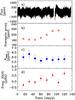 |
Fig. 2 a) Flux of HD 49385 as a function of time (starting October 18, 2007) measured by CoRoT (only 1 point every 5 has been plotted). b) starspot proxy computed as described in Sect. 2. c) temporal variation of the maximum amplitude per radial mode with their associated error bar. d) temporal variation of the averaged frequency shift of the p modes. In panels b), c), and d), only every other point is independent. |
The temporal evolution of the maximum amplitude and of the averaged frequency shift of the acoustic modes are shown in Figs. 2c and d.
When comparing these trends visually, we see an anti-correlation between both parameters: Amax, which slightly decreases and the averaged frequency shift, which presents a slight increase during the observations. According to what we know of the Sun and HD 49933, a situation like this corresponds to a small increase in the activity level of the star, which is corroborated by the surface activity measured by the starspot proxy (see Fig. 2b). The correlation coefficient was computed using the Spearmans rank correlation on independent points alone (one over two, starting with the first one). We chose the rank correlation because the two variables are not expected to have a linear relationship. This analysis confirms that there is an anti-correlation between the two signals but the numerical value is low (−0.4, see Table 3). The high value of the false-alarm probability associated to the correlation coefficient indicates that the anti-correlation has not been firmly detected.
The spectropolarimetric observations of HD 49385 are constituted of four spectra collected between December 21, 2008 and April 13, 2009, i.e. one year after the CoRoT observations. Over this timespan, we observe a low-level chromospheric flux, with an average value of the chromospheric index equal to 0.139 (see Table 2). The measured temporal fluctuations of the chromospheric emission are not statistically significant. The polarised spectra provide us with an upper limit of about 1 Gauss on the line-of-sight magnetic field component. This analysis is compatible with a general low-activity period. This result combined with the seismic observations do not allow us to make a firm detection of any magnetic modulation in this star. However, HD 49385 will deserve to be revisited with CoRoT during the extension of the mission to confirm the tendency unveiled here. It would be the first subgiant with an on-going magnetic-activity cycle seismically observed.
Chromospheric emission in the core of the Ca ii H spectral line.
Spearmans correlation coefficients of Amax and the averaged frequency shifts using only the independent points (one over two) starting by the first one and its associated false-alarm probability.
3.2. HD 181420
HD 181420 is an F2 star with Teff = 6580 ± 105 K. The projected rotational velocity vsini = 18 ± 1 km s-1 (see Bruntt 2009, for a detailed description of the spectroscopic properties of this star). The surface rotation period, derived from the light curve observed by CoRoT, was estimated by Barban et al. (2009) to be around 2.6 days with an important surface differential rotation. This yields – in combination with the vsini given previously – an inclination angle for the star of 35 ± 21°. With the wavelet analysis, we also find this main periodicity (Fig. 3). The WPS shows a broad peak confirming the presence of an important differential rotation at the surface of the star. Moreover, there is no signature of any other harmonic at longer periods.
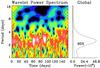 |
Fig. 3 WPS (left) and GWPS (right) of HD 181420 (same legend as in Fig. 1). Observations started on May 11, 2007. |
The temporal evolution of the averaged frequency shift and Amax are shown in Figs. 4c and d. Amax shows a small modulation, while the averaged frequency shift exhibits flat behaviour (excepting the last point). It is no surprise that the correlation of the independent points of the two signals is weak with the same sign, making a small correlation of 0.3 and a false-alarm probability close to 60% (see Table 3).
When we analyse the light curve, in both the WPS and the starspot proxy, we see an increase in the signal around the sixtieth and the eightieth days of the measurements. This region of higher surface activity corresponds to the small maximum we observe in Amax, which is not what we expect if this is an activity effect. We can conclude from the seismic analysis that we do not see any change related to a magnetic activity modulation in this star, while in the light curve we do see the starspots (see Fig. 4a).
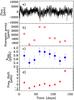 |
Fig. 4 Analysis of HD 181420. Same legend as in Fig. 2. Observations started on May 11, 2007. In panels b), c), and d), only every other point is independent. |
Spectropolarimetric data for HD 181420 were collected between June 2, 2007 and July 15, 2008, and they overlap slightly with the asteroseismic data. Over this period, the average chromospheric index was equal to 0.245, with values ranging from 0.227 and 0.265 (see Table 2). The observed temporal fluctuations do not reveal a long-term trend. In spite of a chromospheric flux higher than solar, the signal-to-noise ratio of the polarised spectra is not sufficient for the detection of Zeeman signatures because of a significant rotational broadening of the line profile. We infer an upper limit of about 3 Gauss on the line-of-sight magnetic field component.
3.3. HD 52265
HD 52265 is a G0V, metal-rich, main-sequence star hosting a planet (Butler et al. 2000; Naef et al. 2001). Its effective temperature is Teff = 6100 ± 60 K, and the projected rotational velocity is  km s-1 (see Ballot et al. 2011, for a complete review of the stellar parameters and the seismic analysis). Using the measurements provided by CoRoT – during 117 continuous days starting on November 13, 2008, we determined the rotation rate of the star: Prot = 12.3 ± 0.15 days, with a stellar inclination angle of 30 ± 10°.
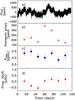 |
Fig. 5 Analysis of HD 52265. Same legend as in Fig. 2. Observations started in November 13, 2008. In panels b), c), and d), only every other point is independent. |
The visual inspection of the averaged frequency shift and Amax – plotted in Figs. 5c and d – presents very small variations. This is confirmed by the cross correlation coefficient which is of the order of +0.4, indicating that both signals are not anti-correlated (see Table 3). Once again the non-negligible false-alarm probability does not support the correlation between the two quantities.
The starspot proxy (Fig. 5b) presents an increase around the middle of the data set. We notice that in the light curve displayed in Fig. 5a, there is indeed a sudden increase in the flux around that period. Although we cannot rule out a stellar origin, this kind of modulation is often due to instrumental instabilities in the CoRoT satellite and should then be treated with some precaution.
Our spectropolarimetric observations of HD 52265 were obtained between December 20, 2008 and January 11, 2009, i.e. the first part was collected during the CoRoT observations. From these time series, we derive an average chromospheric index of 0.159 (see Table 2), with a slight increase over the observing run, which is visible in Fig. 6. Here again, the noise level in the polarised spectra remains too high to reach the detection threshold of Zeeman signatures, which can at least allow us to place a tight upper limit of 0.6 Gauss on the longitudinal component of its large-scale photospheric field.
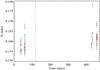 |
Fig. 6 Chromospheric emission of the Ca ii H line measured at different epochs with NARVAL for HD 52265. Grey points are the individual measurements, while the red ones correspond to the daily averages. The starting date of the time series coincides with the beginning of CoRoT observations, i.e. November 13, 2008. The end of CoRoT observations is delineated with a vertical dashed line. |
4. Discussion and conclusion
In the present paper we have performed an extended analysis of seismic and spectroscopic data using CoRoT and NARVAL to look for signatures of magnetic activity cycles in three stars: HD 49385, HD 181420, and HD 52265. The seismic analysis was done by studying the temporal variation of the maximum amplitude of the modes, Amax and of the averaged frequency shifts, while the spectroscopic analysis consisted of measurements in Ca H chromospheric emission lines and we also researched for any Zeeman polarised signatures.
The information that we can extract from this analysis is limited by the data we have in hand and the length of the observations. Indeed, we only have seven or eight data points and in each case, two consecutive points are correlated because of an overlap between the subseries analysed.
Given the limitation of our analysis related to the length of the observations, we require that three criteria are fulfilled to be able to firmly detect magnetic modulations with our analysis. The amplitude of the modes and their frequency shifts must show a temporal variation. These two parameters have to be anti-correlated. Finally, we should observe a temporal variation in the spectroscopic data correlated with the seismic quantities.
For all the stars the seismic indicators show very small variations, which are, in general compatible with no variation at all at a 2-σ level. Only HD 49385 presents an anti-correlation between the two parameters, suggesting a rising phase of a possible magnetic activity cycle but with a small correlation coefficient (~−40%) and a false-alarm probability of ~50%. No confirmation could be done with the spectropolarimetric measurements. Nevertheless we infer an upper limit of the line-of-sight magnetic field component of 1 G. Therefore, these results prevent us from concluding that we detected any magnetic modulation in this star.
For the other two stars, HD 181420 and HD 52265, the correlation between the two seismic indicators has a positive sign and is lower then 40%, ruling out the existence of a magnetic modulation on this time scale. However, HD 52265 shows a small increase in the S-index (using two sets of observations separated by about one year). This could indicate a change in magnetic activity towards a maximum of activity. However, since we do not have any variation in the seismic indicators we cannot claim for any firm detection of any magnetic activity change. The upper limit of the line-of-sight magnetic field component obtained was 3 G for HD 181420 and 0.6 G for HD 52265.
In conclusion, the analysis presented here established that if there are any magnetic activity cycles in these stars, they would be longer than the CoRoT observation period of ~120 days, which is a limiting factor. The false-alarm probabilities of the correlation coefficients are too high to confirm any trend. Moreover, through the spectroscopic analysis we can say that for HD 52265, the lower limit could be about a year, but this should be taken with caution because the magnitude of the variation measured is very small.
Longer datasets will be needed to further investigate the presence of magnetic cycles in stars other than the Sun. This could be soon possible thanks to the data collected by the Kepler satellite or by revisiting these stars with CoRoT in the incoming years during the extension of the mission.
Acknowledgments
The CoRoT space mission has been developed and is operated by CNES, with contributions from Austria, Belgium, Brazil, ESA (RSSD and Science Program), Germany and Spain. NARVAL is a collaborative project funded by France (Région Midi-Pyrénées, CNRS, MENESR, Conseil Général des Hautes Pyrénées) and the European Union (FEDER funds). D.S. acknowledges the financial support from CNES. J.B., R.A.G., S.M., A.M., and P.P. acknowledge the support given by the French “Programme National de Physique Stellaire”. RAG also acknowledges the CNES for the support of the CoRoT activities at the SAp, CEA/Saclay. This research has been partially supported by the Spanish Ministry of Science and Innovation (MICINN) under the grant AYA2010-20982-C02-02.NCAR is supported by the National Science Foundation. Wavelet software was provided by C. Torrence and G. Compo, and is available at URL: http://paos.colorado.edu/research/wavelets/.
References
- Anderson, E. R., Duvall, Jr., T. L., & Jefferies, S. M. 1990, ApJ, 364, 699 [NASA ADS] [CrossRef] [Google Scholar]
- Anguera Gubau, M., Palle, P. L., Perez Hernandez, F., Regulo, C., & Roca Cortes, T. 1992, A&A, 255, 363 [NASA ADS] [Google Scholar]
- Aurière, M. 2003, in EAS Publ. Ser. 9, eds. J. Arnaud, & N. Meunier, 105 [Google Scholar]
- Baglin, A., Auvergne, M., Barge, P., et al. 2006, in ESA SP 1306, eds. M. Fridlund, A. Baglin, J. Lochard, & L. Conroy, 33 [Google Scholar]
- Baliunas, S. L., & Vaughan, A. H. 1985, ARA&A, 23, 379 [NASA ADS] [CrossRef] [Google Scholar]
- Baliunas, S. L., Donahue, R. A., Soon, W. H., et al. 1995, ApJ, 438, 269 [NASA ADS] [CrossRef] [Google Scholar]
- Ballot, J., Gizon, L., Samadi, R., et al. 2011, A&A, 530, A97 [NASA ADS] [CrossRef] [EDP Sciences] [Google Scholar]
- Barban, C., Deheuvels, S., Baudin, F., et al. 2009, A&A, 506, 51 [NASA ADS] [CrossRef] [EDP Sciences] [Google Scholar]
- Batalha, N. M., Jenkins, J., Basri, G. S., Borucki, W. J., & Koch, D. G. 2002, in Stellar Structure and Habitable Planet Finding, eds. B. Battrick, F. Favata, I. W. Roxburgh, & D. Galadi, ESA SP, 485, 35 [Google Scholar]
- Beer, J., Tobias, S., & Weiss, N. 1998, Sol. Phys., 181, 237 [Google Scholar]
- Böhm-Vitense, E. 2007, ApJ, 657, 486 [NASA ADS] [CrossRef] [Google Scholar]
- Borucki, W. J., Koch, D., Basri, G., et al. 2010, Science, 327, 977 [NASA ADS] [CrossRef] [PubMed] [Google Scholar]
- Browning, M. K., Miesch, M. S., Brun, A. S., & Toomre, J. 2006, ApJ, 648, L157 [Google Scholar]
- Bruntt, H. 2009, A&A, 506, 235 [NASA ADS] [CrossRef] [EDP Sciences] [Google Scholar]
- Butler, R. P., Vogt, S. S., Marcy, G. W., et al. 2000, ApJ, 545, 504 [NASA ADS] [CrossRef] [Google Scholar]
- Chaplin, W. J., Appourchaux, T., Elsworth, Y., Isaak, G. R., & New, R. 2001, MNRAS, 324, 910 [NASA ADS] [CrossRef] [Google Scholar]
- Chaplin, W. J., Bedding, T. R., Bonanno, A., et al. 2011a, ApJ, 732, L5 [Google Scholar]
- Chaplin, W. J., Kjeldsen, H., Christensen-Dalsgaard, J., et al. 2011b, Science, 332, 213 [NASA ADS] [CrossRef] [PubMed] [Google Scholar]
- Deheuvels, S., & Michel, E. 2011, A&A, 535, A91 [NASA ADS] [CrossRef] [EDP Sciences] [Google Scholar]
- Deheuvels, S., Bruntt, H., Michel, E., et al. 2010, A&A, 515, A87 [NASA ADS] [CrossRef] [EDP Sciences] [Google Scholar]
- Donati, J., Semel, M., Carter, B. D., Rees, D. E., & Collier Cameron, A. 1997, MNRAS, 291, 658 [NASA ADS] [CrossRef] [MathSciNet] [Google Scholar]
- Fares, R., Donati, J.-F., Moutou, C., et al. 2009, MNRAS, 398, 1383 [NASA ADS] [CrossRef] [MathSciNet] [Google Scholar]
- Fletcher, S., New, R., Broomhall, A.-M., Chaplin, W., & Elsworth, Y. 2010, in SOHO-23: Understanding a Peculiar Solar Minimum, eds. S. R. Cranmer, J. T. Hoeksema, & J. L. Kohl, ASP Conf. Ser., 428, 43 [Google Scholar]
- Gabriel, A. H., Grec, G., Charra, J., et al. 1995, Sol. Phys., 162, 61 [NASA ADS] [CrossRef] [Google Scholar]
- García, R. A., Turck-Chièze, S., Boumier, P., et al. 2005, A&A, 442, 385 [NASA ADS] [CrossRef] [EDP Sciences] [Google Scholar]
- García, R. A., Mathur, S., Salabert, D., et al. 2010, Science, 329, 1032 [NASA ADS] [CrossRef] [PubMed] [Google Scholar]
- Goldreich, P., Murray, N., Willette, G., & Kumar, P. 1991, ApJ, 370, 752 [NASA ADS] [CrossRef] [Google Scholar]
- Hall, J. C., Lockwood, G. W., & Skiff, B. A. 2007, AJ, 133, 862 [NASA ADS] [CrossRef] [Google Scholar]
- Harvey, J. 1985, in Future Missions in Solar, Heliospheric & Space Plasma Physics, eds. E. Rolfe, & B. Battrick, ESA SP, 235, 199 [Google Scholar]
- Hekker, S., Elsworth, Y., De Ridder, J., et al. 2011, A&A, 525, A131 [NASA ADS] [CrossRef] [EDP Sciences] [Google Scholar]
- Huber, D., Bedding, T. R., Stello, D., et al. 2010, ApJ, 723, 1607 [NASA ADS] [CrossRef] [Google Scholar]
- Huber, D., Bedding, T. R., Stello, D., et al. 2011, ApJ, 743, 143 [NASA ADS] [CrossRef] [Google Scholar]
- Jiménez-Reyes, S. J., Chaplin, W. J., Elsworth, Y., & García, R. A. 2004, ApJ, 604, 969 [NASA ADS] [CrossRef] [Google Scholar]
- Kjeldsen, H., & Bedding, T. R. 1995, A&A, 293, 87 [NASA ADS] [Google Scholar]
- Kjeldsen, H., Bedding, T. R., Arentoft, T., et al. 2008, ApJ, 682, 1370 [NASA ADS] [CrossRef] [Google Scholar]
- Lanza, A. F. 2010, in IAU Symp. 264, eds. A. G. Kosovichev, A. H. Andrei, & J.-P. Roelot, 120 [Google Scholar]
- Liu, Y., Liang, X., & Weisberg, R. 2007, Atmos. Ocean Tech., 24, 2093 [Google Scholar]
- Mathur, S., García, R. A., Catala, C., et al. 2010a, A&A, 518, A53 [NASA ADS] [CrossRef] [EDP Sciences] [Google Scholar]
- Mathur, S., García, R. A., Régulo, C., et al. 2010b, A&A, 511, A46 [NASA ADS] [CrossRef] [EDP Sciences] [Google Scholar]
- Mathur, S., Handberg, R., Campante, T. L., et al. 2011a, ApJ, 733, 95 [NASA ADS] [CrossRef] [Google Scholar]
- Mathur, S., Hekker, S., Trampedach, R., et al. 2011b, ApJ, 741, 119 [NASA ADS] [CrossRef] [Google Scholar]
- Mathur, S., Metcalfe, T. S., Woitaszek, M., et al. 2012, ApJ, 749, 152 [NASA ADS] [CrossRef] [Google Scholar]
- Metcalfe, T. S., Creevey, O. L., & Christensen-Dalsgaard, J. 2009, ApJ, 699, 373 [NASA ADS] [CrossRef] [Google Scholar]
- Metcalfe, T. S., Basu, S., Henry, T. J., et al. 2010, ApJ, 723, L213 [NASA ADS] [CrossRef] [Google Scholar]
- Michel, E., Baglin, A., Auvergne, M., et al. 2008, Science, 322, 558 [NASA ADS] [CrossRef] [PubMed] [Google Scholar]
- Michel, E., Samadi, R., Baudin, F., et al. 2009, A&A, 495, 979 [NASA ADS] [CrossRef] [EDP Sciences] [Google Scholar]
- Mosser, B., Baudin, F., Lanza, A. F., et al. 2009, A&A, 506, 245 [NASA ADS] [CrossRef] [EDP Sciences] [Google Scholar]
- Mosser, B., Elsworth, Y., Hekker, S., et al. 2012, A&A, 537, A30 [NASA ADS] [CrossRef] [EDP Sciences] [Google Scholar]
- Naef, D., Mayor, M., Pepe, F., et al. 2001, A&A, 375, 205 [NASA ADS] [CrossRef] [EDP Sciences] [Google Scholar]
- Pallé, P. L., Regulo, C., & Roca Cortes, T. 1989, A&A, 224, 253 [NASA ADS] [Google Scholar]
- Petit, P., Dintrans, B., Solanki, S. K., et al. 2008, MNRAS, 388, 80 [NASA ADS] [CrossRef] [MathSciNet] [Google Scholar]
- Petit, P., Dintrans, B., Morgenthaler, A., et al. 2009, A&A, 508, L9 [NASA ADS] [CrossRef] [EDP Sciences] [Google Scholar]
- Rees, D. E., & Semel, M. D. 1979, A&A, 74, 1 [NASA ADS] [Google Scholar]
- Ribas, I., Porto de Mello, G. F., Ferreira, L. D., et al. 2010, ApJ, 714, 384 [NASA ADS] [CrossRef] [Google Scholar]
- Saar, S. H., & Brandenburg, A. 1999, ApJ, 524, 295 [NASA ADS] [CrossRef] [Google Scholar]
- Salabert, D., Fossat, E., Gelly, B., et al. 2004, A&A, 413, 1135 [NASA ADS] [CrossRef] [EDP Sciences] [Google Scholar]
- Salabert, D., García, R. A., Pallé, P. L., & Jiménez-Reyes, S. J. 2009, A&A, 504, L1 [NASA ADS] [CrossRef] [EDP Sciences] [Google Scholar]
- Salabert, D., Ballot, J., & García, R. A. 2011a, A&A, 528, A25 [NASA ADS] [CrossRef] [EDP Sciences] [Google Scholar]
- Salabert, D., Régulo, C., Ballot, J., García, R. A., & Mathur, S. 2011b, A&A, 530, A127 [NASA ADS] [CrossRef] [EDP Sciences] [Google Scholar]
- Skumanich, A. 1972, ApJ, 171, 565 [NASA ADS] [CrossRef] [Google Scholar]
- Strassmeier, K. G. 2009, in IAU Symp., 259, 363 [Google Scholar]
- Torrence, C., & Compo, G. P. 1998, Bull. Am. Meteor. Soc., 79, 61 [Google Scholar]
- Vázquez Ramió, H., Mathur, S., Régulo, C., & García, R. A. 2011, J. Phys. Conf. Ser., 271, 012056 [NASA ADS] [CrossRef] [Google Scholar]
- Verner, G. A., Elsworth, Y., Chaplin, W. J., et al. 2011, MNRAS, 415, 3539 [NASA ADS] [CrossRef] [Google Scholar]
- Wilson, O. C. 1978, ApJ, 226, 379 [NASA ADS] [CrossRef] [Google Scholar]
- Woodard, M. F., & Noyes, R. W. 1985, Nature, 318, 449 [NASA ADS] [CrossRef] [Google Scholar]
- Wright, J. T., Marcy, G. W., Butler, R. P., & Vogt, S. S. 2004, ApJS, 152, 261 [NASA ADS] [CrossRef] [Google Scholar]
All Tables
Frequency range used to compute the averaged frequency shift and Amax of the 3 stars.
Spearmans correlation coefficients of Amax and the averaged frequency shifts using only the independent points (one over two) starting by the first one and its associated false-alarm probability.
All Figures
|
Fig. 1 Left panel: wavelet power spectrum (WPS) as a function of time of HD 49385. The origin of time is October 18, 2007. Right panel: global WPS (GWPS). The shaded region in the WPS corresponds to the cone of influence, i.e. the region in which the periods cannot be analysed due to the short length of the observations. |
| In the text | |
|
Fig. 2 a) Flux of HD 49385 as a function of time (starting October 18, 2007) measured by CoRoT (only 1 point every 5 has been plotted). b) starspot proxy computed as described in Sect. 2. c) temporal variation of the maximum amplitude per radial mode with their associated error bar. d) temporal variation of the averaged frequency shift of the p modes. In panels b), c), and d), only every other point is independent. |
| In the text | |
|
Fig. 3 WPS (left) and GWPS (right) of HD 181420 (same legend as in Fig. 1). Observations started on May 11, 2007. |
| In the text | |
|
Fig. 4 Analysis of HD 181420. Same legend as in Fig. 2. Observations started on May 11, 2007. In panels b), c), and d), only every other point is independent. |
| In the text | |
|
Fig. 5 Analysis of HD 52265. Same legend as in Fig. 2. Observations started in November 13, 2008. In panels b), c), and d), only every other point is independent. |
| In the text | |
|
Fig. 6 Chromospheric emission of the Ca ii H line measured at different epochs with NARVAL for HD 52265. Grey points are the individual measurements, while the red ones correspond to the daily averages. The starting date of the time series coincides with the beginning of CoRoT observations, i.e. November 13, 2008. The end of CoRoT observations is delineated with a vertical dashed line. |
| In the text | |
Current usage metrics show cumulative count of Article Views (full-text article views including HTML views, PDF and ePub downloads, according to the available data) and Abstracts Views on Vision4Press platform.
Data correspond to usage on the plateform after 2015. The current usage metrics is available 48-96 hours after online publication and is updated daily on week days.
Initial download of the metrics may take a while.