| Issue |
A&A
Volume 549, January 2013
|
|
|---|---|---|
| Article Number | A113 | |
| Number of page(s) | 9 | |
| Section | The Sun | |
| DOI | https://doi.org/10.1051/0004-6361/201220272 | |
| Published online | 08 January 2013 | |
Torsional Alfvén waves in partially ionized solar plasma: effects of neutral helium and stratification
1
Space Research Institute, Austrian Academy of Sciences,
Schmiedlstrasse 6,
8042
Graz,
Austria
e-mail: teimuraz.zaqarashvili@oeaw.ac.at; maxim.khodachenko@oeaw.ac.at
2
Departament de Física, Universitat de les Illes
Balears, 07122
Palma de Mallorca,
Spain
e-mail: roberto.soler@uib.es
3
Abastumani Astrophysical Observatory at Ilia State University,
University St. 2, 1060
Tbilisi,
Georgia
Received:
22
August
2012
Accepted:
14
November
2012
Context. Ion-neutral collisions may lead to the damping of Alfvén waves in chromospheric and prominence plasmas. Neutral helium atoms enhance the damping in certain temperature intervals, where the ratio of neutral helium and neutral hydrogen atoms is increased. Therefore, the height dependence of the ionization degrees of hydrogen and helium may influence the damping rate of Alfvén waves.
Aims. We aim to study the effect of neutral helium on the damping of Alfvén waves in stratified, partially ionized plasma of the solar chromosphere.
Methods. We consider a magnetic flux tube, which is expanded up to 1000 km height and then becomes vertical owing to merging with neighboring tubes, and study the dynamics of linear torsional Alfvén waves in the presence of neutral hydrogen and neutral helium atoms. We start with a three-fluid description of plasma and subsequently derive single-fluid magnetohydrodynamic (MHD) equations for torsional Alfvén waves. Thin flux tube approximation allows us to obtain the dispersion relation of the waves in the lower part of tubes, while the spatial dependence of steady-state Alfvén waves is governed by a Bessel-type equation in the upper parts of the tubes.
Results. Consecutive derivation of single-fluid MHD equations results in a new Cowling diffusion coefficient in the presence of neutral helium, which is different from the previously used one. We find that shorter period (<5 s) torsional Alfvén waves damp quickly in the chromospheric network owing to ion-neutral collision. On the other hand, longer period (>5 s) waves do not reach the transition region because they become evanescent at lower heights in the network cores.
Conclusions. Propagation of torsional Alfvén waves through the chromosphere into the solar corona should be considered with caution: low-frequency waves are evanescent owing to the stratification, while high-frequency waves are damped by ion-neutral collisions.
Key words: Sun: atmosphere / Sun: oscillations
© ESO, 2013
1. Introduction
Alfvén waves play an important role in the dynamics of the solar atmosphere. Photospheric motions may excite the waves, which then propagate upwards along the anchored magnetic field and transport the energy into upper layers, where they may deposit the energy back leading to the chromospheric/coronal heating and/or the acceleration of solar wind particles. The photospheric magnetic field is concentrated in flux tubes, which are very dynamic and may continuously change shape and/or merge because of granular motions. Nevertheless, in a crude representation useful for theoretical modeling, the magnetic field can be approximated as axis-symmetric tubes, therefore the excited pure Alfvén waves are axis-symmetric; i.e. they are torsional Alfvén waves. If considering a cylindrically symmetric flux tube, torsional waves correspond to the azimuthal wavenumber set to m = 0 in the standard notation. On the other hand, granular buffeting may excite transverse magnetohydrodynamic (MHD) kink waves in the tubes, which then can be transformed into linearly polarized Alfvén waves in the upper layer thanks to the expansion of tubes (Cranmer & van Ballegooijen 2005). The transverse oscillations have been observed with both imaging and spectroscopic observations (Kukhianidze et al. 2006; Zaqarashvili et al. 2007; De Pontieu et al. 2007, the interested reader may find a detailed review of oscillations in Zaqarashvili & Erdélyi 2009).
Torsional Alfvén waves do not lead to the displacement of magnetic tube axis, therefore they can only be observed with spectroscopic observations as a periodic variation in spectral line width (Zaqarashvili 2003). Observations of torsional Alfvén waves have been recently reported in chromospheric spectral lines (Jess et al. 2009; De Pontieu et al. 2012). Upward propagating undamped Alfvén waves can also be observed in the solar corona as an increase in nonthermal broadening of coronal spectral lines with height (Hassler et al. 1990).
The dynamics of Alfvén waves in the chromosphere/corona and their role in plasma heating have been studied quite well (Hollweg 1981; 1984; Copil et al. 2008; Antolin & Shibata 2010; Vasheghani Farahani et al. 2010; 2011; Morton et al. 2011). They can be excited by the vortex motion at the photospheric level (Fedun et al. 2011a). In the case of inhomogeneous plasma, Alfvén waves may also be excited by resonances with other wave modes (see, e.g., Soler et al. 2012). Torsional Alfvén waves can be used as supplementary tool for solar magnetoseismology (Zaqarashvili & Murawski 2007; Verth et al. 2010; Fedun et al. 2011b).
In the solar chromosphere and prominences, plasma is only partially ionized, which leads to damping of Alfvén waves owing to collision between ions and neutral hydrogen atoms (De Pontieu et al. 2001; Khodachenko et al. 2004; Leake et al. 2005; Forteza et al. 2007; Soler et al. 2009; Carbonell et al. 2010; Singh & Krishan 2010). Upward propagating Alfvén waves may also drive spicules through ion-neutral collisions (Haerendel 1992; James & Erdélyi 2002; Erdélyi & James 2004).
Single-fluid MHD description is a good approximation for low-frequency waves, but it fails when the wave frequency approaches an ion-neutral collision frequency, and consequently the multi-fluid MHD description should be used. It was shown by Zaqarashvili et al. (2011a) that the damping rate is maximum for the waves those frequency is near an ion-neutral collision frequency; i.e., higher and lower frequency waves have less damping rates.
Besides the neutral hydrogen atoms, the solar plasma may contain significant amount of neutral helium atoms, which may enhance the damping of Alfvén waves. Soler et al. (2010) suggested that the neutral helium has no significant influence on the damping rate in the prominence cores with 8000 K temperature. On the other hand, Zaqarashvili et al. (2011b) showed that the neutral helium may significantly enhance the damping of Alfvén waves in the temperature interval of 10 000−40 000 K, where the ratio of neutral helium and neutral hydrogen atoms is increased. This means that the helium atoms can be important in upper chromosphere, spicules, and prominence-corona transition regions. The neutral helium effects in Zaqarashvili et al. (2011b) was calculated in a homogeneous medium with uniform magnetic field and ionization degree. On the other hand, the ion and neutral atom number densities, hence ionization degree, are significantly changed with height in the chromosphere, which may influence the damping of Alfvén waves due to ion-neutral collisions.
Stratification may significantly influence the dynamics of waves, leading to their reflection in the transition region, mutual transformation, and/or evanescence. It introduces a cut-off frequency for Alfvén waves in fully ionized plasma; i.e., waves with lower frequency than the cut-off value are evanescent in the solar atmosphere (Musielak et al. 1995; Murawski & Musielak 2010).
In this paper, we study the effects of stratification and neutral helium atoms on the propagation/damping of Alfvén waves in the solar chromosphere. We consider a magnetic flux tube, which is expanded up to 1000 km height and then becomes vertical owing to merging with neighboring tubes. Consequently, we consider torsional Alfvén waves, which are only purely incompressible waves in tubes.
2. Linear torsional Alfvén waves
We consider a vertical magnetic flux tube embedded in the stratified solar atmosphere. We
use cylindrical coordinate system (r,θ,z) and suppose that the unperturbed
magnetic field, B0, is untwisted i.e.
B0θ = 0. Plasma consists in electrons,
protons (H + ), singly ionized helium (He + ), neutral hydrogen (H),
and neutral helium (He) atoms. We consider the Alfvén waves polarized in θ
direction; i.e., the only non-zero components of the perturbations are
vθ and
bθ. Therefore, the waves are torsional
Alfvén waves. We start with the three-fluid approach for partially ionized hydrogen-helium
plasma, when one component is ion + electron gas and the other two components are neutral
hydrogen and neutral helium gasses (Zaqarashvili et al. 2011b). Then, the linear Alfvén waves are governed by the following equations
(magnetic diffusion due to ion-electron collision is neglected): 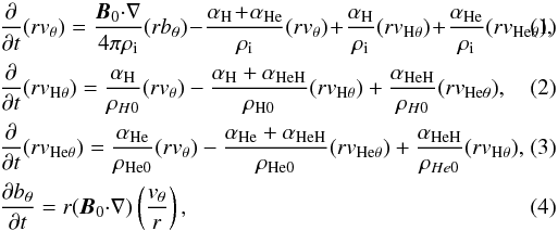 \arraycolsep1.75ptwhere
vθ
(vHθ,
vHeθ) are the perturbations of ion (neutral
hydrogen, neutral helium) velocity, bθ is the
perturbation of the magnetic field, and ρi
(ρH0, ρHe0) is the unperturbed ion
(neutral hydrogen, neutral helium) density. Here we use the definitions
\arraycolsep1.75ptwhere
vθ
(vHθ,
vHeθ) are the perturbations of ion (neutral
hydrogen, neutral helium) velocity, bθ is the
perturbation of the magnetic field, and ρi
(ρH0, ρHe0) is the unperturbed ion
(neutral hydrogen, neutral helium) density. Here we use the definitions  (5)where
α denotes the coefficient of friction between different sorts of species.
The collision between electrons and neutral atoms is also neglected since it has much less
of an effect on the damping of MHD waves than the collision between ions and neutrals. In
the present model the motions of torsional Alfvén waves are normal to the direction of
gravity, so that gravity does not explicitly appear in the equations. The effect of gravity
is indirectly present in the equations through the stratification of plasma density.
(5)where
α denotes the coefficient of friction between different sorts of species.
The collision between electrons and neutral atoms is also neglected since it has much less
of an effect on the damping of MHD waves than the collision between ions and neutrals. In
the present model the motions of torsional Alfvén waves are normal to the direction of
gravity, so that gravity does not explicitly appear in the equations. The effect of gravity
is indirectly present in the equations through the stratification of plasma density.
The coefficient of friction between ions and neutrals (in the case of same temperature) is
calculated as (Braginskii 1965) 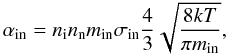 (6)where T is
the plasma temperature, mi (mn) the
ion (neutral atom) mass,
min = mimn/(mi + mn)
is reduced mass, ni (nn) is the ion
(neutral atom) number density,
(6)where T is
the plasma temperature, mi (mn) the
ion (neutral atom) mass,
min = mimn/(mi + mn)
is reduced mass, ni (nn) is the ion
(neutral atom) number density, 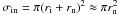 is the
ion-neutral collision cross section for direct, elastic collisions from Braginskii (1965) (mean atomic cross section is
is the
ion-neutral collision cross section for direct, elastic collisions from Braginskii (1965) (mean atomic cross section is
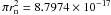 cm2),
and k = 1.38 × 10⁻¹⁶ erg K-1 is the Boltzmann
constant.
cm2),
and k = 1.38 × 10⁻¹⁶ erg K-1 is the Boltzmann
constant.
From here we adopt the single-fluid approximation. To justify whether or not the
single-fluid approximation is valid in the solar atmosphere we estimate the ion-neutral
collision frequency. Mean collision frequency between ions and neutrals can be calculated as
(Zaqarashvili et al. 2011b)  (7)The collision frequency is
very high in the photosphere and decreases upwards. For example, The collision frequency
between protons and neutral hydrogen can be estimated as 8.6 × 10⁶ Hz,
6.2 × 10³ Hz, and 24 Hz, at z = 0,
z = 900 km, and z = 1900 km correspondingly. Ion and
neutral atom number densities were taken from Fontenla et al. (1993, model-F). Therefore, the Alfvén waves with periods >1 s
can be studied in the single-fluid approach.
(7)The collision frequency is
very high in the photosphere and decreases upwards. For example, The collision frequency
between protons and neutral hydrogen can be estimated as 8.6 × 10⁶ Hz,
6.2 × 10³ Hz, and 24 Hz, at z = 0,
z = 900 km, and z = 1900 km correspondingly. Ion and
neutral atom number densities were taken from Fontenla et al. (1993, model-F). Therefore, the Alfvén waves with periods >1 s
can be studied in the single-fluid approach.
To obtain the governing equations in the single-fluid approximation, we consider the total
density  (8)and the
velocity of center of mass
(8)and the
velocity of center of mass 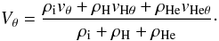 (9)We also consider the
relative velocity of ion and neutral hydrogen as
wHθ = vθ − vHθ
and the relative velocity of ion and neutral helium as
wHeθ = vθ − vHeθ.
Then one may find that
(9)We also consider the
relative velocity of ion and neutral hydrogen as
wHθ = vθ − vHθ
and the relative velocity of ion and neutral helium as
wHeθ = vθ − vHeθ.
Then one may find that  (10)where
ξH = ρH/ρ and
ξHe = ρHe/ρ.
(10)where
ξH = ρH/ρ and
ξHe = ρHe/ρ.
Consecutive substraction of Eqs. (1)
and (2), Eqs. (1) and (3), Eqs. (2) and (3) and neglecting the inertial terms for relative
velocities lead to the equations ![\begin{eqnarray} \label{w_H1} rw_{\mathrm {H}\theta}&=&\left [{{\alpha_{\rm He}}\over {\alpha}}\xi_{\rm H}+{{\alpha_{\rm HeH}}\over {\alpha}}(\xi_{\rm H}+\xi_{\rm He})\right ]{\vec B_0{\cdot}\nabla\over {4 \pi}}(rb_{\theta}), \\ \label{w_He1} rw_{\rm He}&=&\left [{{\alpha_{\rm H}}\over {\alpha}}\xi_{\rm He}+{{\alpha_{\rm HeH}}\over {\alpha}}(\xi_{\rm H}+\xi_{\rm He})\right ]{\vec B_0{\cdot}\nabla\over {4 \pi}}(rb_{\theta}), \end{eqnarray}](/articles/aa/full_html/2013/01/aa20272-12/aa20272-12-eq48.png) where
α = αHαHe + αHαHeH + αHeαHeH.
Neglecting the inertial terms is justified for waves whose frequency is less than the
ion-neutral collision frequency. This is the key step in transforming the multi fluid
equations into the single fluid description.
where
α = αHαHe + αHαHeH + αHeαHeH.
Neglecting the inertial terms is justified for waves whose frequency is less than the
ion-neutral collision frequency. This is the key step in transforming the multi fluid
equations into the single fluid description.
Then the sum of Eqs. (1)−(3) and use of Eqs. (4), (10)−(12) lead to the single-fluid equations
![\begin{eqnarray} \label{eqs1} &&{{\partial }\over {\partial t}}(rV_{\theta})= {\vec B_0{\cdot}\nabla\over {4 \pi \rho(z)}}(rb_{\theta}), \\ \label{eqs2} &&{{\partial b_{\theta}}\over {\partial t}}=r(\vec B_0{\cdot}\nabla)\left ({{V_{\theta}}\over {r}}\right ) +r(\vec B_0{\cdot}\nabla)\left [ {{\eta_{\rm c}(z)}\over {B^2_0}} {\vec B_0{\cdot}\nabla\over {r^2}}(rb_{\theta})\right ], \end{eqnarray}](/articles/aa/full_html/2013/01/aa20272-12/aa20272-12-eq50.png) where
where
 (15)is
the coefficient of Cowling diffusion. The first two terms in the nominator of Eq. (15) are due the frictions of neutral hydrogen
and neutral helium separately with regard to ions, while the last term is the friction of
neutral hydrogen+helium fluid with regards to ions. Therefore, the last term is important in
weakly ionized plasmas, while the first two terms are important for a relatively high value
for the ionization degree. Soler et al. (2010) used
the following expression for Cowling diffusion in the presence of neutral helium
(15)is
the coefficient of Cowling diffusion. The first two terms in the nominator of Eq. (15) are due the frictions of neutral hydrogen
and neutral helium separately with regard to ions, while the last term is the friction of
neutral hydrogen+helium fluid with regards to ions. Therefore, the last term is important in
weakly ionized plasmas, while the first two terms are important for a relatively high value
for the ionization degree. Soler et al. (2010) used
the following expression for Cowling diffusion in the presence of neutral helium
 (16)which can be obtained from
our expression (Eq. (15))
when αH,αHe ≪ αHeH,
i.e., when plasma is only weakly ionized. This is so because in their derivation Soler
et al. (2010) considered that both neutral hydrogen
and neutral helium have the same velocity. That is equivalent to takeing
αHeH → ∞. Therefore the present description is more general
than that of Soler et al. (2010). The expression used
by Soler et al. (2010) is only approximately valid
for the photosphere and lower chromosphere, while the general expression Eq. (15) should be used in the upper chromosphere,
spicules and prominences.
(16)which can be obtained from
our expression (Eq. (15))
when αH,αHe ≪ αHeH,
i.e., when plasma is only weakly ionized. This is so because in their derivation Soler
et al. (2010) considered that both neutral hydrogen
and neutral helium have the same velocity. That is equivalent to takeing
αHeH → ∞. Therefore the present description is more general
than that of Soler et al. (2010). The expression used
by Soler et al. (2010) is only approximately valid
for the photosphere and lower chromosphere, while the general expression Eq. (15) should be used in the upper chromosphere,
spicules and prominences.
We next consider a new coordinate s, which represents a longitudinal
coordinate along the unperturbed magnetic field,
B0. Then Eqs. (13), (14) can be combined
into the single equation in terms of this new coordinate, namely
![\begin{eqnarray} {{\partial^2 {U_{\theta}}}\over {\partial t^2}}&=&{{B_{\rm 0s}}\over {4\pi \rho r^2}} {{\partial }\over {\partial s}}\left [r^2 B_{\rm 0s} {{\partial {U_{\theta}}}\over {\partial s}}\right]\notag\\ &&+{{B_{\rm 0s}}\over {4\pi \rho r^2}} {{\partial }\over {\partial s}}\left [r^2 B_{\rm 0s} {{\partial }\over {\partial s}} \left ({{4\pi \rho \eta_{\rm c}}\over {B^2_{\rm 0s}}}{{\partial {U_{\theta}}}\over {\partial t}} \right )\right ], \end{eqnarray}](/articles/aa/full_html/2013/01/aa20272-12/aa20272-12-eq56.png) (17)where
Uθ = Vθ/r.
We note that r is a function of s. This equation is
simplified near the axis of symmetry, where
B0s(s)r2(s) ≈ const.
(Hollweg 1981), which is the conservation of magnetic
flux near the tube axis, where field lines are almost perpendicular to the tube’s
cross-section. Then this equation may be written as
(17)where
Uθ = Vθ/r.
We note that r is a function of s. This equation is
simplified near the axis of symmetry, where
B0s(s)r2(s) ≈ const.
(Hollweg 1981), which is the conservation of magnetic
flux near the tube axis, where field lines are almost perpendicular to the tube’s
cross-section. Then this equation may be written as ![\begin{equation} \label{eqs4} {{\partial^2 {U_{\theta}}}\over {\partial t^2}}=V^2_{\rm A}(s) {{\partial^2 }\over {\partial s^2}}\left [\left (1+ {{\eta_{\rm c}(s)}\over {V^2_{\rm A}(s)}} {{\partial }\over {\partial t}}\right ){U_{\theta}}\right ], \end{equation}](/articles/aa/full_html/2013/01/aa20272-12/aa20272-12-eq60.png) (18)where
(18)where  (19)is
the Alfvén speed.
(19)is
the Alfvén speed.
Solar atmospheric parameters depend on the height owing to gravity. The plasma ionization degree is also a function of altitude because of the increase in temperature with height. The plasma is only weakly ionized in the photosphere/lower chromosphere. The increase in temperature with height leads to the ionization of hydrogen and helium atoms, which become almost fully ionized in the solar corona, so the transition occurs near the region of a sharp temperature rise.
 |
Fig. 1 Height dependence of atmospheric parameters according to FAL93-F model (Fontenla et al. 1993): magenta, red, and blue lines correspond to proton, neutral helium, and neutral hydrogen number densities, respectively. Green line is the total (proton + neutral hydrogen+neutral helium) number density. |
 |
Fig. 2 Ratio of Cowling diffusion coefficient and Alfvén speed square,
|
Figure 1 shows the density of different species vs. height according to the FAL93-F model (Fontenla et al. 1993). This model includes the dependence of ionization degree on the heights for both hydrogen and helium. The neutral atom number densities are much higher than the ion number densities at the lower heights, but become comparable near ~1900 km, which corresponds to the temperature of about 10 000 K. It is seen that the neutral atoms are more stratified than protons between 500 and 2000 km heights: the neutral hydrogen, neutral helium, and total number densities have scale heights of about 180 km, while the scale height of protons is much greater. The total number density is similar to the neutral hydrogen number density until ~1500 km. Above this height they start to diverge due to the increase in ionization degree.
Fourier analysis of Eq. (18) with
exp [− iωt] , where ω is the wave frequency, gives
the equation ![\begin{equation} \label{strat0} V^2_{\rm A}(s) {{\partial^2 }\over {\partial s^2}}\left[\left(1- {\rm i}{{\omega \eta_{\rm c}(s)}\over {V^2_{\rm A}(s)}}\right){U_{\theta}}\right]+\omega^2 {U_{\theta}}=0, \end{equation}](/articles/aa/full_html/2013/01/aa20272-12/aa20272-12-eq66.png) (20)which governs the spatial
dependence of steady-state torsional Alfvén waves. The type of the equation depends on the
dependence of VA and ηc
on s.
(20)which governs the spatial
dependence of steady-state torsional Alfvén waves. The type of the equation depends on the
dependence of VA and ηc
on s.
A very important parameter in Eq. (20) is
the ratio  , which does not
depend on the magnetic field structure with height because
, which does not
depend on the magnetic field structure with height because
 is canceled. We plot
the ratio vs. height according to the VAL93-F model in Fig. 2. It is clearly seen that the ratio is almost constant throughout the
chromosphere and abruptly increases near the transition region. Therefore, to find
analytical solutions to Eq. (20) we consider
the ratio as a constant along s in the chromosphere
is canceled. We plot
the ratio vs. height according to the VAL93-F model in Fig. 2. It is clearly seen that the ratio is almost constant throughout the
chromosphere and abruptly increases near the transition region. Therefore, to find
analytical solutions to Eq. (20) we consider
the ratio as a constant along s in the chromosphere 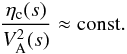 (21)From
Fig. 2 we see that this approximation seems to be
good in the upper part of the chromosphere, i.e., between 800−2000 km, while it may be not
as accurate in the lower part of the chromosphere, i.e., in the interval
between 500−800 km. Nevertheless, we use this approximation in the whole chromosphere for
convenience.
(21)From
Fig. 2 we see that this approximation seems to be
good in the upper part of the chromosphere, i.e., between 800−2000 km, while it may be not
as accurate in the lower part of the chromosphere, i.e., in the interval
between 500−800 km. Nevertheless, we use this approximation in the whole chromosphere for
convenience.
Plasma β (= ) is constant with
height in the isothermal atmosphere in thin vertical magnetic flux tubes, when temperatures
inside and outside the tubes are the same (Roberts 2004). In this case, the Alfvén speed is also constant with height, yielding
VA(s) = VA0 = const.
The constancy of the Alfvén speed in thin tubes is caused by the compensation for density
variation by the magnetic field strength variation with height. The thin flux tube
approximation is valid up to 1000 km above the photosphere (Hasan et al. 2003; Cranmer & van Ballegooijen 2005). Above this height, the magnetic tubes are thick,
and they probably merge with neighboring tubes to produce an almost vertical magnetic field
(Fig. 3). Then, the Alfvén speed may vary with height
owing to the decrease in density, while the magnetic field is constant. According to this
model, we consider the vertical magnetic tube, which consists in two different parts: the
lower part with constant Alfvén speed and the upper part with exponentially increasing
Alfvén speed. Then we study the torsional Alfvén waves in the two parts of magnetic flux
tube separately.
) is constant with
height in the isothermal atmosphere in thin vertical magnetic flux tubes, when temperatures
inside and outside the tubes are the same (Roberts 2004). In this case, the Alfvén speed is also constant with height, yielding
VA(s) = VA0 = const.
The constancy of the Alfvén speed in thin tubes is caused by the compensation for density
variation by the magnetic field strength variation with height. The thin flux tube
approximation is valid up to 1000 km above the photosphere (Hasan et al. 2003; Cranmer & van Ballegooijen 2005). Above this height, the magnetic tubes are thick,
and they probably merge with neighboring tubes to produce an almost vertical magnetic field
(Fig. 3). Then, the Alfvén speed may vary with height
owing to the decrease in density, while the magnetic field is constant. According to this
model, we consider the vertical magnetic tube, which consists in two different parts: the
lower part with constant Alfvén speed and the upper part with exponentially increasing
Alfvén speed. Then we study the torsional Alfvén waves in the two parts of magnetic flux
tube separately.
 |
Fig. 3 Vertical magnetic flux tube model: below 1000 km the Alfvén speed is constant due to the thin flux tube approximation and above 1000 km height the Alfvén speed increases exponentially. |
3. Lower chromosphere: thin flux tube approximation
In the lower part of the magnetic flux tube, the thin tube approximation is used, which
yields VA(s) = const. (see
previous section). The thin tube approximation is still compatible with a magnetic flux tube
expanding with height. The only restriction is that the wavelength remains much longer than
the tube radius. This case was also studied by Soler et al. (2009) for the case of torsional Alfvén waves in prominence threads. The constancy
of Alfvén speed means that the coefficient of Cowling diffusion is also constant. Then the
coefficients of Eq. (20) do not depend on
s, therefore Fourier analysis with
exp [i(kss − ωt)] gives
the dispersion relation  (22)which has two
complex solutions
(22)which has two
complex solutions  (23)The dispersion relation and
its solutions agree with Eqs. (33) and (34) of Soler et al. (2009). The real part of this expression gives the wave frequency, which shows that
there is the cut-off wavenumber due to Cowling’s diffusion,
ks = 2VA/ηc.
The cut-off wave number due to ion-neutral collision was found in different situations of
the solar prominences (Forteza et al. 2007; Soler
et al. 2009; Barcélo et al. 2011). It is the result of approximation when one transforms multifluid
equations into the single-fluid MHD, and therefore it has no physical basis (Zaqarashvili
et al. 2012).
(23)The dispersion relation and
its solutions agree with Eqs. (33) and (34) of Soler et al. (2009). The real part of this expression gives the wave frequency, which shows that
there is the cut-off wavenumber due to Cowling’s diffusion,
ks = 2VA/ηc.
The cut-off wave number due to ion-neutral collision was found in different situations of
the solar prominences (Forteza et al. 2007; Soler
et al. 2009; Barcélo et al. 2011). It is the result of approximation when one transforms multifluid
equations into the single-fluid MHD, and therefore it has no physical basis (Zaqarashvili
et al. 2012).
On the other hand, the imaginary part of this expression gives the normalized damping rate
as 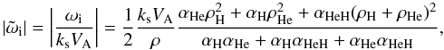 (24)where we have used the full
expression of Cowling’s coefficient, ηc. The plasma is almost
neutral in the low chromosphere, therefore
αHeH ≫ αH,αHe.
This leads to the normalized damping rate
(24)where we have used the full
expression of Cowling’s coefficient, ηc. The plasma is almost
neutral in the low chromosphere, therefore
αHeH ≫ αH,αHe.
This leads to the normalized damping rate ![\begin{equation} \label{damping1} |{\tilde \omega_{\rm i}}|\approx{1\over 2} {{k_{\rm s} V_{\rm A}}\over {\rho}} \left [{{(\rho_{\rm H}+\rho_{\rm He})^2}\over {\alpha_{\rm H}+\alpha_{\rm He}}}\right ]\cdot \end{equation}](/articles/aa/full_html/2013/01/aa20272-12/aa20272-12-eq81.png) (25)This expression was used by
Soler et al. (2010) to calculate the effect of neutral helium in prominence cores.
(25)This expression was used by
Soler et al. (2010) to calculate the effect of neutral helium in prominence cores.
On the other hand, when the number density of neutral atoms is much less than ion number
density, then
αHeH ≪ αH,αHe
and the normalized damping rate is ![\begin{equation} \label{damping2} |{\tilde \omega_{\rm i}}|\approx{1\over 2} {{k_{\rm s} V_{\rm A}}\over {\rho}} \left[{{\rho^2_{\rm H}}\over {\alpha_{\rm H}}}+{{\rho^2_{\rm He}}\over {\alpha_{\rm He}}}\right]\cdot \end{equation}](/articles/aa/full_html/2013/01/aa20272-12/aa20272-12-eq83.png) (26)When ion number density is
similar to the number density of neutral atoms (as in spicules or in prominence cores), then
the general expression of damping rate (Eq. (24)) should be used. The expression Eq. (24) may significantly change the contribution of neutral helium atoms.
(26)When ion number density is
similar to the number density of neutral atoms (as in spicules or in prominence cores), then
the general expression of damping rate (Eq. (24)) should be used. The expression Eq. (24) may significantly change the contribution of neutral helium atoms.
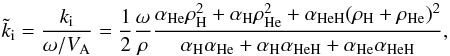
Figure 4 shows the normalized damping time
( )
vs. the period of Alfvén waves
(T0 = 2π/ksVA)
for three different areas: a) FAL93-A corresponding to faint cell center area; b) FAL93-F
corresponding to bright area of chromospheric network; and c) prominence cores. We use the
following parameters: a)
ni = 3.26 × 1010 cm-3,
nH = 3.01 × 1013 cm-3,
nHe = 3.01 × 1012 cm-3 taken from
FAL93-A at 975 km height corresponding to ≈ 5480 K temperature; b)
ni = 2.49 × 1011 cm-3,
nH = 5.24 × 1013 cm-3,
nHe = 5.26 × 1012 cm-3 was taken from
FAL93-F at 975 km height corresponding to 6180 K temperature; and c)
ni = 1010 cm-3,
nH = 2 × 1010 cm-3,
nHe = 2 × 109 cm-3 was taken for
prominence cores corresponding to 8000 K temperature. It is clearly seen that the presence
of neutral helium atoms significantly enhances the damping of Alfvén waves. It is also seen
that the damping of torsional Alfvén waves is more efficient in the faint cell center area
in the chromosphere and in prominence cores, where the waves are damped over a few wave
periods. On the other hand, the damping of torsional Alfvén waves due to ion-neutral
collision is inefficient in the bright chromospheric network center. The clear difference in
damping in these two areas can be understood in terms of the ion-neutral collision
frequency. In the absence of neutral helium atoms, Eq. (24) can be rewritten as (Zaqarashvili et al. 2011b)
)
vs. the period of Alfvén waves
(T0 = 2π/ksVA)
for three different areas: a) FAL93-A corresponding to faint cell center area; b) FAL93-F
corresponding to bright area of chromospheric network; and c) prominence cores. We use the
following parameters: a)
ni = 3.26 × 1010 cm-3,
nH = 3.01 × 1013 cm-3,
nHe = 3.01 × 1012 cm-3 taken from
FAL93-A at 975 km height corresponding to ≈ 5480 K temperature; b)
ni = 2.49 × 1011 cm-3,
nH = 5.24 × 1013 cm-3,
nHe = 5.26 × 1012 cm-3 was taken from
FAL93-F at 975 km height corresponding to 6180 K temperature; and c)
ni = 1010 cm-3,
nH = 2 × 1010 cm-3,
nHe = 2 × 109 cm-3 was taken for
prominence cores corresponding to 8000 K temperature. It is clearly seen that the presence
of neutral helium atoms significantly enhances the damping of Alfvén waves. It is also seen
that the damping of torsional Alfvén waves is more efficient in the faint cell center area
in the chromosphere and in prominence cores, where the waves are damped over a few wave
periods. On the other hand, the damping of torsional Alfvén waves due to ion-neutral
collision is inefficient in the bright chromospheric network center. The clear difference in
damping in these two areas can be understood in terms of the ion-neutral collision
frequency. In the absence of neutral helium atoms, Eq. (24) can be rewritten as (Zaqarashvili et al. 2011b) 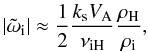 (27)which clearly indicates
that the normalized damping rate depends on the ratio of Alfvén frequency over ion-neutral
hydrogen collision frequency (νiH) and the ratio of neutral and
ion fluid densities. For ρi ≪ ρH,
which is the case at 975 km height, ion-neutral hydrogen collision frequency is proportional
to neutral hydrogen density,
νiH ~ ρH. This means that
the normalized damping rate is inversely proportional to ion number density,
ρi. The proton number density is almost ten times lower in the
cell center than in the network center, which leads to almost ten times difference in
damping (Fig. 4).
(27)which clearly indicates
that the normalized damping rate depends on the ratio of Alfvén frequency over ion-neutral
hydrogen collision frequency (νiH) and the ratio of neutral and
ion fluid densities. For ρi ≪ ρH,
which is the case at 975 km height, ion-neutral hydrogen collision frequency is proportional
to neutral hydrogen density,
νiH ~ ρH. This means that
the normalized damping rate is inversely proportional to ion number density,
ρi. The proton number density is almost ten times lower in the
cell center than in the network center, which leads to almost ten times difference in
damping (Fig. 4).
 |
Fig. 4 Normalized damping time of torsional Alfvén waves (Td/T0) vs. wave period (T0) for three different situations from top to bottom: faint cell center area (FAL93-A), bright network (FAL93-F), and prominence core. The blue line indicates the wave damping due to collision of ions with neutral hydrogen atoms alone. The red line indicates the wave damping due to collision of ions with neutral hydrogen and neutral helium atoms. |
In the first part of this section, we have studied the temporal damping of Alfvén waves,
i.e., we set a real ks and solved the dispersion relation to
obtain the complex ω. In the following paragraphs, we study the spatial
damping. This means that the dispersion relation (Eq. (22)) is now solved for the complex wavenumber,
ks, assuming a fixed and real ω. The solution
of the dispersion relation for the square of ks is 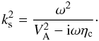 (28)We use this expression to
find the real and imaginary parts of ks, assuming
ks = kr + iki.
After some algebraic manipulations we can obtain the expressions for
(28)We use this expression to
find the real and imaginary parts of ks, assuming
ks = kr + iki.
After some algebraic manipulations we can obtain the expressions for
 and
ki, namely
and
ki, namely 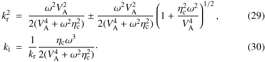 The
expression of kr is computed from Eq. (29) as
The
expression of kr is computed from Eq. (29) as  .
The ± sign in front of the second term in the expression of
leads to four
possible values of kr. The two values of
kr with + sign in the expression of
correspond to
propagating waves, namely
.
The ± sign in front of the second term in the expression of
leads to four
possible values of kr. The two values of
kr with + sign in the expression of
correspond to
propagating waves, namely 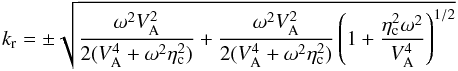 (31)where
the ± sign in front of the square root refers to upward and downward waves.
(31)where
the ± sign in front of the square root refers to upward and downward waves.
To obtain more simplified analytical formulas we consider the case of weak damping; i.e.,
 . The expression of
kr for propagating waves becomes
. The expression of
kr for propagating waves becomes
 (32)We now take the + sign
corresponding to upward propagating waves and use this expression to compute the value of
ki in the limit ,
(32)We now take the + sign
corresponding to upward propagating waves and use this expression to compute the value of
ki in the limit ,
 (33)The corresponding
normalized damping rate using the full expression of ηc is
(33)The corresponding
normalized damping rate using the full expression of ηc is
 (34)which is equivalent to
Eq. (24) obtained for the temporal damping
if we replace ω by
ksVA. Therefore, both spatial and
temporal damping rates of the Alfvén waves are equivalent.
(34)which is equivalent to
Eq. (24) obtained for the temporal damping
if we replace ω by
ksVA. Therefore, both spatial and
temporal damping rates of the Alfvén waves are equivalent.
 |
Fig. 5 Height dependence of steady-state, torsional Alfvén waves with periods of 5 s. Green
line corresponds to |
On the other hand, the two values of kr corresponding to
the−sign in the expression of (Eq. (29)) correspond to evanescent waves,
 (35)which for weak damping,
i.e., , becomes
(35)which for weak damping,
i.e., , becomes
 (36)This corresponds to
evanescent perturbations that do not propagate from the location of the excitation, so these
solutions are not relevant for the present study.
(36)This corresponds to
evanescent perturbations that do not propagate from the location of the excitation, so these
solutions are not relevant for the present study.
4. Upper chromosphere: exponentially increasing Alfvén speed
In the upper part of magnetic flux tube, where the neighboring tubes are merged, we assume
that the Alfvén speed is exponentially increasing (the ratio of Cowling diffusion
coefficient and Alfvén speed square is assumed to be constant again), 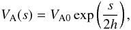 (37)where h is
the scale height and VA0 corresponds to the value of Alfvén
speed at the height of 1000 km (i.e., s = 0 also corresponds to the height
of 1000 km). In this case, Eq. (20) can be
rewritten as
(37)where h is
the scale height and VA0 corresponds to the value of Alfvén
speed at the height of 1000 km (i.e., s = 0 also corresponds to the height
of 1000 km). In this case, Eq. (20) can be
rewritten as 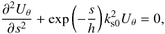 (38)where
 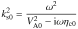 (39)and
ηc0 is the value of Cowling diffusion at the height of
1000 km. The solution of this equation is
(39)and
ηc0 is the value of Cowling diffusion at the height of
1000 km. The solution of this equation is 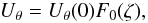 (40)where
F0 is Bessel, modified Bessel or Hankel functions of zero
order and
(40)where
F0 is Bessel, modified Bessel or Hankel functions of zero
order and
![$$ \zeta=2hk_{\rm s0}\exp\left [{-{s\over {2h}}}\right ]\cdot $$](/articles/aa/full_html/2013/01/aa20272-12/aa20272-12-eq132.png) Propagating waves are
described by Hankel functions (
Propagating waves are
described by Hankel functions ( ,
,
 ), and
standing waves are described by Bessel functions
(J0(ζ)).
), and
standing waves are described by Bessel functions
(J0(ζ)).
 and
and
 functions have the same spatial
dependence in the case of fully ionized plasma (Fig. 5). The upward and downward propagating waves can be distinguished by the sign of
time-averaged Pointing flux (Hollweg 1984), which
shows that is upward-propagating and
is downward-propagating waves. In
the case of partially ionized plasma distinguishing between upward and downward propagating
waves is complicated by the complex argument of Hankel functions (De Pontieu et al. 2001). However, it is still possible to distinguish them
by a careful look into the height structure of waves (Fig. 5). has smaller amplitude at higher
heights in partially ionized case compared to the fully ionized case, while
has the stronger amplitude. This
means that governs the wave, which damps at
higher heights owing to ion-neutral collisions, therefore it governs the dynamics of
upwardly propagating waves. On the same basis, governs the downwardly
propagating waves. The standing waves, expressed by
J0(ζ), can be formed after superposition of
upward- and downward-propagating waves.
functions have the same spatial
dependence in the case of fully ionized plasma (Fig. 5). The upward and downward propagating waves can be distinguished by the sign of
time-averaged Pointing flux (Hollweg 1984), which
shows that is upward-propagating and
is downward-propagating waves. In
the case of partially ionized plasma distinguishing between upward and downward propagating
waves is complicated by the complex argument of Hankel functions (De Pontieu et al. 2001). However, it is still possible to distinguish them
by a careful look into the height structure of waves (Fig. 5). has smaller amplitude at higher
heights in partially ionized case compared to the fully ionized case, while
has the stronger amplitude. This
means that governs the wave, which damps at
higher heights owing to ion-neutral collisions, therefore it governs the dynamics of
upwardly propagating waves. On the same basis, governs the downwardly
propagating waves. The standing waves, expressed by
J0(ζ), can be formed after superposition of
upward- and downward-propagating waves.
A mathematical proof that the function  corresponds to
upward waves is obtained from the asymptotic expansion of the Hankel functions for large
arguments (see, e.g., Stenuit et al. 1999). For large
ζ, which eventually means small s, the dependence of
Hankel functions on s can be written as
corresponds to
upward waves is obtained from the asymptotic expansion of the Hankel functions for large
arguments (see, e.g., Stenuit et al. 1999). For large
ζ, which eventually means small s, the dependence of
Hankel functions on s can be written as
 where
ks0 is given in Eq. (39). These expansions clearly show that corresponds to
upwardly propagating waves when the temporal dependence is exp [− iωt] .
In the rest of the paper we only consider upwardly propagating waves. Only the real parts of
and
, i.e., the part of the solution
with the physical meaning, are shown in all plots.
where
ks0 is given in Eq. (39). These expansions clearly show that corresponds to
upwardly propagating waves when the temporal dependence is exp [− iωt] .
In the rest of the paper we only consider upwardly propagating waves. Only the real parts of
and
, i.e., the part of the solution
with the physical meaning, are shown in all plots.
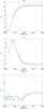 |
Fig. 6 Height dependence of steady-state, upward propagating torsional Alfvén waves with periods of 20 s (upper panel), 10 s (middle panel), and 3 s (lower panel). Green lines correspond to the fully ionized plasma, and blue (red) lines correspond to partially ionized plasma with neutral hydrogen atoms (neutral hydrogen + neutral helium atoms). |
Figure 6 shows the height dependence of upward propagating torsional Alfvén waves with different periods in the bright chromospheric network cores. At a 1000 km height we use the number densities from the FAL93-F model such as ni = 3.22 × 1011 cm-3, nH = 2.65 × 1013 cm-3, and nHe = 2.68 × 1012 cm-3. The plasma temperature is set as T = 8000 K and the Alfvén speed as VA0 = 20 km s-1. It is seen that the behavior of longer period waves (>10 s) is not significantly affected by ion-neutral collisions: the height dependence is similar for fully ionized and partially ionized plasmas (upper panel). The shorter period waves display more significant dependence on ion-neutral collisions. For example, the torsional Alfvén waves with periods of 3 s are significantly damped in partially ionized plasma compared to the fully ionized case (lower panel). It is also seen that the presence of neutral helium enhances the damping of Alfvén waves compared to neutral hydrogen only. Figure 6 shows that the spatial dependence of waves is not oscillatory above particular heights; i.e., waves become evanescent. To study this phenomenon, we consider wave propagation in fully ionized plasma.
Figure 7 displays the velocity of torsional Alfvén waves vs. height for different wave periods. It is seen that torsional Alfvén waves with periods of 20 s become evanescent above a 1500 km height. Waves with 5 s periods become evanescent above a 1800 km height, but the waves with 1 s periods penetrate up to a 2600 km height. Therefore, the longer period waves (>5 s) do not reach transition region (2000 km height), but become evanescent at lower heights. This gravitational cut-off of Alfvén waves has been known for a long time (Musielak & Moore 1995). Recently, Murawski & Musielak (2010) have also shown that the linearly polarized Alfvén waves become evanescent above some heights in fully ionized plasma. Our result confirms their analyses.
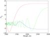 |
Fig. 7 Height dependence of steady-state, upward-propagating torsional Alfvén waves with periods of 20 s (red line), 5 s (blue line), and 1 s (green line) in fully ionized plasma. |
5. Discussion
Propagation of Alfvén waves in the chromosphere is very important for chromospheric/coronal heating because they may carry the photospheric energy into the upper layers. The magnetic field is concentrated in flux tubes at the photospheric level, therefore the torsional Alfvén waves can be generated by vortex motions (Fedun et al. 2011a). Observation of torsional Alfvén waves is possible through the periodic variation in spectral line width (Zaqarashvili 2003). Recently, Jess et al. (2009) have reported the observation of torsional Alfvén waves in the lower chromosphere. The energy flux carried by the waves was enough to heat the solar corona. Therefore, it is interesting to study whether the waves may penetrate the corona.
Here we study the torsional Alfvén waves in chromospheric magnetic flux tubes with partially ionized plasma taking neutral hydrogen and neutral helium atoms into account. We consider the stratification due to gravity, therefore the tubes are expanding with height. Hasan et al. (2003) showed that the magnetic flux tubes can be considered as thin up to a 1000 km height from the surface. Above this height, the neighboring magnetic flux tubes merge and the field lines are almost vertical. We use this model and split the magnetic tubes into two layers. We use the expanding thin flux tube approximation in the lower chromosphere below 1000 km. In the upper layer, above 1000 km we consider the magnetic field lines as vertical, so only medium density changes with height. We use the FAL93 model (Fontenla et al. 1993) for the dependence of ion, neutral hydrogen, and neutral helium number densities with height.
We start with a three-fluid MHD description of partially ionized plasma, where one component is electron-proton-singly ionized helium and the other two components are neutral hydrogen and neutral helium gasses. Then we proceed to the single-fluid description by standard procedures and neglect the inertial terms of ion-neutral hydrogen and ion-neutral helium relative velocities. We obtain the Cowling diffusion coefficient (Eq. (15)), which is different from the previously used one. Namely, the expression Eq. (15) contains additional terms (the first and second terms in nominator) that express the collision of ions with neutral hydrogen and neutral helium atoms separately. The previously used expression of the Cowling diffusion coefficient is valid in weakly ionized plasma, where the coupling between neutral atoms is stronger.
In the lower part of magnetic flux tube, where the thin tube approximations is used, the dispersion relation for the torsional Alfvén waves is obtained. The solution of the dispersion relation shows that the damping of Alfvén waves due to ion-neutral collision is significant in faint cell center areas at all frequencies, while only high-frequency waves are damped in the chromospheric network cores (Fig. 4). This means that torsional Alfvén waves may propagate without any problem up to 1000 km above the surface in chromospheric network cores. The effect of neutral helium atoms is significant in all cases, and it increases for lower frequency waves.
In the upper part of magnetic flux tube, the height dependence of torsional Alfvén wave
velocity is governed by a Bessel-type equation, therefore the solutions are Bessel or Hankel
functions with zero-order and complex arguments. We consider only upward propagating waves,
which are expressed by Hankel functions, . The solution
of steady-state torsional Alfvén waves shows that the long-period waves are not affected by
ion-neutral collisions. Only short-period waves (<5 s) are damped significantly
(Fig. 6). The existence of neutral helium atoms
enhances damping of the waves but not significantly. On the other hand, long-period waves
show no oscillatory behavior above certain heights, so they become evanescent in the upper
part of the chromosphere. This phenomenon is called gravitational cut-off (Musielak et al.
1995; Murawski & Musielak 2010). It is seen that only the waves with very short
periods (~1 s) may reach the transition region and corona in the case of fully
ionized plasma (Fig. 7). This means that the
low-frequency waves cannot reach the transition region due to the gravitational cut-off, but
high-frequency waves are damped due to ion-neutral collision. Then the torsional Alfvén
waves cannot reach the transition region at all. This is true near the axis of magnetic flux
tubes, where our approximations are valid. However, it is possible that some wave tunneling
exists there, and the evanescent tail of the waves can indeed reach the transition region
and the corona. Owing to the change in the ambient conditions, the waves may propagate again
in the corona. In the outer part of tubes, where magnetic field lines are more inclined, the
problem of wave propagation along the chromosphere may not arise at all. This requires
further detailed study.
On the other hand, Alfvén waves may easily penetrate the corona if they are excited in the higher part of the chromosphere (Hansen & Cally 2012). Long-period acoustic oscillations (p-modes) are evanescent in the lower atmosphere owing to the gravitational stratification; however, they may propagate with an angle about the vertical and may trigger Alfvén waves in the upper chromosphere through mode conversion (Zaqarashvili & Roberts 2006; Cally & Goossens 2008; Cally & Hansen 2011; Khomenko & Cally 2012). If low-frequency torsional Alfvén waves are excited above a 1000 km height, then our model also allows the propagation of the waves into the corona since the evanescent point can be shifted up above the transition region (Fig. 7).
Recently, Vranjes et al. (2008) have suggested that the energy flux of Alfvén waves excited in the photosphere is overestimated, and thus the Alfvén waves can hardly be excited in the photosphere (but see Tsap et al. 2011, for alternative point of view). This is indeed an interesting question that should be addressed adequately. One possible explanation is that Vranjes et al. (2008) considered the magnetic field strength of 100 G in the photosphere, which is too weak for flux tubes, where the magnetic field strength is of order kG. Therefore, it is possible that the Alfvén waves are excited only inside flux tubes, but not outside the tubes, where the magnetic field is relatively weak. This point needs further discussion.
Ion-neutral collisions are only important for short-period waves (<5 s). On the other hand, only long-period transverse oscillations (≥ 3 min) have so far been observed frequently in the solar atmosphere. However, some observations from ground based coronagraphs show the oscillations of spicule axes with periods of ≤ 1 min (Zaqarashvili et al. 2007; Zaqarashvili & Erdélyi 2009). Several reasons could explain the absence of high-frequency oscillations: not enough tempo-spatial resolution of observations, hard excitation in the photospheric level, quick damping in the lower atmosphere, etc. We hope that more sophisticated observations will help us improve our knowledge about high-frequency oscillations in the future.
6. Conclusions
Propagation of torsional Alfvén waves along expanding vertical magnetic flux tubes in the partially ionized solar chromosphere was studied, the ion collisions with neutral hydrogen and neutral helium atoms taking into account. The waves propagate freely in the lower chromosphere up to 1000 km and may be damped by ion-neutral collisions. The new expression of the Cowling diffusion (and consequently damping rate) including the neutral helium was obtained (Eq. (15)). Neutral helium atoms may significantly enhance the damping of Alfvén waves. On the other hand, the long-period (>5 s) waves propagating near the tube axis become evanescent above some height in the upper chromosphere and do not reach the transition region, while the short-period waves (<5 s) are damped by ion-neutral collisions. As a result, the torsional Alfvén waves may not reach the transition region and the corona, unless some tunneling effects are considered. This means that the coronal heating by photospheric Alfvén waves should be considered with caution. At the same time, energy of the waves can be dissipated in the chromosphere, leading to the heating of ambient plasma.
Acknowledgments
The work was supported by the Austrian Fonds zur Förderung der wissenschaftlichen Forschung (project P21197-N16) and by the European FP7-PEOPLE-2010-IRSES-269299 project-SOLSPANET. R.S. acknowledges support from a Marie Curie Intra-European Fellowship within the European Commission 7th Framework Program (PIEF-GA-2010-274716). R.S. also acknowledges support from MINECO and FEDER funds through project AYA2011-22846 and from CAIB through the “Grups Competitius” scheme.
References
- Antolin, P., & Shibata, K. 2010, ApJ, 712, 494 [NASA ADS] [CrossRef] [Google Scholar]
- Barcélo, S., Carbonell, M., & Ballester, J. L. 2011, A&A, 525, A60 [NASA ADS] [CrossRef] [EDP Sciences] [Google Scholar]
- Braginskii, S. I. 1965, Rev. Plasma Phys., 1, 205 [NASA ADS] [Google Scholar]
- Cally, P. S., & Goossens, M. 2008, Sol. Phys., 251, 251 [NASA ADS] [CrossRef] [Google Scholar]
- Cally, P. S., & Hansen, S. C. 2011, ApJ, 738, 119 [NASA ADS] [CrossRef] [Google Scholar]
- Carbonell, M., Forteza, P., Oliver, R., & Ballester, J. L. 2010, A&A, 515, A80 [NASA ADS] [CrossRef] [EDP Sciences] [Google Scholar]
- Copil, P., Voitenko, Y., & Goossens, M. 2008, A&A, 478, 921 [NASA ADS] [CrossRef] [EDP Sciences] [Google Scholar]
- Cranmer, S. R., & van Ballegooijen, A. A. 2005, ApJ, 156, 265 [Google Scholar]
- De Pontieu, B., Martens, P. C. H., & Hudson, H. S. 2001, ApJ, 558, 859 [NASA ADS] [CrossRef] [Google Scholar]
- De Pontieu, B., McIntosh, S. W., Carlsson, M., et al. 2007, Science, 318, 1574 [NASA ADS] [CrossRef] [PubMed] [Google Scholar]
- De Pontieu, B., Carlsson, M., Rouppe van der Voort, L. H. M., et al. 2012, ApJ, 752, L12 [NASA ADS] [CrossRef] [Google Scholar]
- Erdélyi, R., & James, S. P. 2004, A&A, 427, 1055 [NASA ADS] [CrossRef] [EDP Sciences] [Google Scholar]
- Fedun, V., Shelyag, S., Verth, G., Mathioudakis, M., & Erdélyi, R. 2011a, Ann. Geophys., 29, 1029 [Google Scholar]
- Fedun, V., Verth, G., Jess, D. B., & Erdélyi, R. 2011b, ApJ, 740, L46 [NASA ADS] [CrossRef] [Google Scholar]
- Fontenla, J. M., Avrett, E. H., & Loeser, R. 1993, ApJ, 406, 319 [NASA ADS] [CrossRef] [Google Scholar]
- Forteza, P., Oliver, R., Ballester, J. L., & Khodachenko, M. L. 2007, A&A, 461, 731 [NASA ADS] [CrossRef] [EDP Sciences] [Google Scholar]
- Haerendel, G. 1992, Nature, 360, 241 [NASA ADS] [CrossRef] [Google Scholar]
- Hansen, S. C., & Cally, P. S. 2012, ApJ, 751, 31 [NASA ADS] [CrossRef] [Google Scholar]
- Hasan, S. S., Kalkofen, W., van Ballegooijen, A. A., & Ulmschneider, P. 2003, ApJ, 585, 1138 [NASA ADS] [CrossRef] [Google Scholar]
- Hassler, D. M., Rottman, G. J., Shoub, E. C., & Holzer, T. E. 1990, ApJ, 348, L77 [NASA ADS] [CrossRef] [Google Scholar]
- Hollweg, J. V. 1981, Sol. Phys., 70, 25 [NASA ADS] [CrossRef] [Google Scholar]
- Hollweg, J. V. 1984, ApJ, 277, 392 [NASA ADS] [CrossRef] [Google Scholar]
- James, S. P., & Erdélyi, R. 2002, A&A, 393, L11 [NASA ADS] [CrossRef] [EDP Sciences] [Google Scholar]
- Jess, D. B., Mathioudakis, M., Erdïlyi, R., et al. 2009, Science, 323, 1582 [NASA ADS] [CrossRef] [PubMed] [Google Scholar]
- Kukhianidze, V., Zaqarashvili, T. V., & Khutsishvili, E. 2006, A&A, 449, L35 [Google Scholar]
- Khodachenko, M. L. Arber, T. D., Rucker, H. O., & Hanslmeier, A. 2004, A&A, 422, 1073 [NASA ADS] [CrossRef] [EDP Sciences] [Google Scholar]
- Khomenko, E., & Cally, P. S. 2012, ApJ, 746, 68 [NASA ADS] [CrossRef] [Google Scholar]
- Leake, J. E., Arber, T. D., & Khodachenko, M. L. 2005, A&A, 442, 1091 [NASA ADS] [CrossRef] [EDP Sciences] [Google Scholar]
- Morton, R. J., Ruderman, M. S., & Erdélyi, R. 2011, A&A, 534, A27 [NASA ADS] [CrossRef] [EDP Sciences] [Google Scholar]
- Murawski, K., & Musielak, Z. E. 2010, A&A, 518, A37 [NASA ADS] [CrossRef] [EDP Sciences] [Google Scholar]
- Musielak, Z. E., & Moore, R. J. 1995, ApJ, 452, 434 [NASA ADS] [CrossRef] [Google Scholar]
- Roberts, B. 2004, Proc. SOHO 13 – Waves, Oscillations and Small-Scale Transient Events in the Solar Atmosphere: A Joint View from SOHO and TRACE, ESA SP-547, 1 [Google Scholar]
- Singh, K. A. P., & Krishan, V. 2010, New Astron., 15, 119 [NASA ADS] [CrossRef] [Google Scholar]
- Soler, R., Oliver, R., & Ballester, J. L. 2009, ApJ, 699, 1553 [NASA ADS] [CrossRef] [Google Scholar]
- Soler, R., Oliver, R., & Ballester, J. L. 2010, A&A, 512, A28 [NASA ADS] [CrossRef] [EDP Sciences] [Google Scholar]
- Soler, R., Andries, J., & Goossens, M. 2012, A&A, 537, A84 [NASA ADS] [CrossRef] [EDP Sciences] [Google Scholar]
- Stenuit, H., Tirry, W. J., Keppens, R., & Goossens, M. 1999, A&A, 342, 863 [NASA ADS] [Google Scholar]
- Tsap, Y. T., Stepanov, A. V., & Kopylova, Y. G. 2011, Sol. Phys., 270, 205 [NASA ADS] [CrossRef] [Google Scholar]
- VasheghaniFarahani, S., Nakariakov, V. M., & van Doorsselaere, T. 2010, A&A, 517, A29 [NASA ADS] [CrossRef] [EDP Sciences] [Google Scholar]
- Vasheghani Farahani, S., Nakariakov, V. M., van Doorsselaere, T., & Verwichte, E. 2011, A&A, 526, A80 [NASA ADS] [CrossRef] [EDP Sciences] [Google Scholar]
- Verth, G., Erdélyi, R., & Goossens, M. 2010, ApJ, 714, 1637 [NASA ADS] [CrossRef] [Google Scholar]
- Vranjes, J., Poedts, S., Pandey, B. P., & de Pontieu, B. 2008, A&A, 478, 553 [NASA ADS] [CrossRef] [EDP Sciences] [Google Scholar]
- Zaqarashvili, T. V. 2003, A&A, 399, L15 [NASA ADS] [CrossRef] [EDP Sciences] [Google Scholar]
- Zaqarashvili, T. V., & Erdélyi, R. 2009, Space Sci. Rev., 149, 355 [NASA ADS] [CrossRef] [Google Scholar]
- Zaqarashvili, T. V., & Murawski, K. 2007, A&A, 470, 353 [NASA ADS] [CrossRef] [EDP Sciences] [Google Scholar]
- Zaqarashvili, T. V., & Roberts, B. 2006, A&A, 452, 1053 [NASA ADS] [CrossRef] [EDP Sciences] [Google Scholar]
- Zaqarashvili, T. V., Khutsishvili, E., Kukhianidze, V., & Ramishvili, G. 2007, A&A, 474, 627 [NASA ADS] [CrossRef] [EDP Sciences] [Google Scholar]
- Zaqarashvili, T. V., Khodachenko, M. L., & Rucker, H. O. 2011a, A&A, 529, A82 [NASA ADS] [CrossRef] [EDP Sciences] [Google Scholar]
- Zaqarashvili, T. V., Khodachenko, M. L., & Rucker, H. O. 2011b, A&A, 534, A93 [NASA ADS] [CrossRef] [EDP Sciences] [Google Scholar]
- Zaqarashvili, T. V., Carbonell, M., Ballester, J. L., & Khodachenko, M. L. 2012, A&A, 544, A143 [NASA ADS] [CrossRef] [EDP Sciences] [Google Scholar]
All Figures
|
Fig. 1 Height dependence of atmospheric parameters according to FAL93-F model (Fontenla et al. 1993): magenta, red, and blue lines correspond to proton, neutral helium, and neutral hydrogen number densities, respectively. Green line is the total (proton + neutral hydrogen+neutral helium) number density. |
| In the text | |
|
Fig. 2 Ratio of Cowling diffusion coefficient and Alfvén speed square,
|
| In the text | |
|
Fig. 3 Vertical magnetic flux tube model: below 1000 km the Alfvén speed is constant due to the thin flux tube approximation and above 1000 km height the Alfvén speed increases exponentially. |
| In the text | |
|
Fig. 4 Normalized damping time of torsional Alfvén waves (Td/T0) vs. wave period (T0) for three different situations from top to bottom: faint cell center area (FAL93-A), bright network (FAL93-F), and prominence core. The blue line indicates the wave damping due to collision of ions with neutral hydrogen atoms alone. The red line indicates the wave damping due to collision of ions with neutral hydrogen and neutral helium atoms. |
| In the text | |
|
Fig. 5 Height dependence of steady-state, torsional Alfvén waves with periods of 5 s. Green
line corresponds to |
| In the text | |
|
Fig. 6 Height dependence of steady-state, upward propagating torsional Alfvén waves with periods of 20 s (upper panel), 10 s (middle panel), and 3 s (lower panel). Green lines correspond to the fully ionized plasma, and blue (red) lines correspond to partially ionized plasma with neutral hydrogen atoms (neutral hydrogen + neutral helium atoms). |
| In the text | |
|
Fig. 7 Height dependence of steady-state, upward-propagating torsional Alfvén waves with periods of 20 s (red line), 5 s (blue line), and 1 s (green line) in fully ionized plasma. |
| In the text | |
Current usage metrics show cumulative count of Article Views (full-text article views including HTML views, PDF and ePub downloads, according to the available data) and Abstracts Views on Vision4Press platform.
Data correspond to usage on the plateform after 2015. The current usage metrics is available 48-96 hours after online publication and is updated daily on week days.
Initial download of the metrics may take a while.