| Issue |
A&A
Volume 549, January 2013
|
|
|---|---|---|
| Article Number | A89 | |
| Number of page(s) | 11 | |
| Section | Galactic structure, stellar clusters and populations | |
| DOI | https://doi.org/10.1051/0004-6361/201220008 | |
| Published online | 03 January 2013 | |
Approximate integrals of motion
1
Observatoire Astronomique de Strasbourg, UMR 7550 CNRS/Université de
Strasbourg,
Strasbourg,
France
e-mail: This email address is being protected from spambots. You need JavaScript enabled to view it.
2
University of Ljubljana, Faculty of Mathematics and Physics,
Slovenia
Received: 13 July 2012
Accepted: 14 November 2012
Abstract
We determine approximate numerical integrals of motion of 2D symmetric Hamiltonian systems. We detail for a few gravitational potentials the conditions under which quasi-integrals are obtained as polynomial series. We show that each of these potentials has a wide range of regular orbits that are accurately modelled with a unique approximate integral of motion.
Key words: gravitation / methods: numerical / galaxies: kinematics and dynamics
© ESO, 2013
1. Introduction
Gravitational potentials with explicitly known second integrals of motion are rare, the most frequently used in astronomy are axisymmetric potentials and also Stäckel (1893) potentials1 that cover a large class of potentials, but are not always sufficiently realistic. Such explicit forms are useful, for instance, to understand more clearly the underlying physics of dynamical systems, to build stationary distribution functions, etc. Hietarinta (1987) gives such a list of other potentials with known second integrals, but potentials with an analytic second integral of motion are the exception as shown by Poincaré, and ergodic motions should be the rule. However, according to the KAM theorem, at low energies many orbits are regular and remain confined on tori, while for irregular orbits the time diffusion may be exponentially long (Nekhoroshev 1977; Morbidelli & Giorgilli 1995a,b). For these orbits, as shown numerically by Ollongren (1962) for a realistic galactic potential, we expect the existence of approximate first integrals.
The need for generality leads to numerous efforts to obtain tractable integrals of motion for more realistic potentials. Among the developed methods, we can mention the dynamical spectra and more specifically the frequency analysis (Binney & Spergel 1982; Laskar 1993) with a recent 3D application to numerical simulations of galaxies (Valluri et al. 2012). Frequencies associated to each orbit are constants of motion and allow accurate classifications of orbits. Another example, closer to the work developed here, is the tori reconstruction of McGill & Binney (1990), who modelled the tori on which orbits circulate in the phase space. Their analysis is based on the angle-action variables, and the time dependency remains explicit. This method is very attractive since the dynamics of the system becomes very simple. They distort analytic tori of a toy Hamiltonian into the tori of the Hamiltonian of interest. This allows the analysis of any non-integrable potential as a perturbation of a nearly integrable one (Binney & Kumar 1993). Extensions for the separate modelling of orbit families are described by Kaasalainen & Binney (1994), Kaasalainen (1994, 1995). More direct modellings of orbits are also proposed by Prendergast (1982) using the ratio of trigonometric functions, or by Robnik (1993) using Padé approximations (rational functions). Close to our work, Warnock (1991) determined approximate integrals by fitting orbits. He developed a fit using an approximate discrete Fourier transform of positions along orbits and recovered the coefficients of an integral of motion. This method works for non-resonant or high-order resonant orbits but fails for low-order resonant orbits. Bazzani et al. (1991) determined an approximate integral for (2D) sympletic maps, minimising the variation of the approximate integral along the orbit under study.
Formal integrals of motion can be obtained by directly solving the Boltzmann equation assuming that the integral may be written as a polynomial (see Contopoulos 1960). The convergence of these series is not guaranted, but they may be asymptotic (i.e. semi convergent series), allowing one to approximate integrals. Birkhoff (1927) and Gustavson (1966), using normal forms, proposed a process to build such approximate formal integrals of motions. A more complete description of all these subjects can be found in Contopoulos (2002). Introductory lectures on these questions of galactic dynamics and celestial mechanics may be found in Hénon (1983) or Efthymiopoulos et al. (2007).
The motivation of the work presented in this paper is to obtain tractable and approximate integrals of motion for a few simple potentials that are representative of galactic potentials. We restricted our study to 2D motions. Future applications might be the building of dynamically self-consistent galactic models for stationary potentials, and modelling the kinematics of its stellar populations with distribution functions. These goals are usually achieved with N-body numerical simulations, with the Schwarzschild (1979), or with the Syer & Tremaine (1996) methods.
Our method consists of solving the stationary Boltzmann equation for a second integral of motion. Instead of using a formal integration, we numerically determine the coefficients of a series by a least-squares minimisation of the integral variance along orbits. This allows us to obtain a single expression for different orbit families. The method is described in Sect. 2 and detailed explanations and discussion for a simple 2D potential are given in Sect. 3. Applications to other potentials are briefly described in Sects. 4, 5, and the conclusion is presented in Sect. 6.
2. Method and algorithm
According to a definition proposed by Hietarinta (1987), the concept of integrability is to be able to make some quantitative general statements of the dynamical system under study using a quantity whose value is conserved during the time evolution of a system.
In this paper we approach this problem numerically and consider two degrees of freedom time independent Hamiltonian systems of the form  with x,y the space coordinates and u,v their conjugate momenta. The energy is naturally a first invariant, and we search numerically for a second invariant
  independent of the energy.
We recall that this problem is closely related to the collisionless Bolztmann equation and that any distribution function independent of time of the form f(x,v) = g(I(x,v),E(x,v)) will be the solution of the stationary 2D Boltzmann equation, 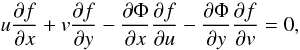 since this equation is also the Poisson bracket { f,H } = 0 that is a property satisfied by any invariant of the Hamiltonian systems.
From Hamilton’s equations of motion, we can determine orbits and note that if a second invariant I(x,v) independent of the energy exists, it remains constant, by definition, along any regular orbit. Thus we assume the existence of such a second invariant, and we also assume that it may be written as a polynomial finite series of the coordinates and momenta (x,y,u,v): 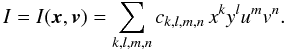 (1)To determine the coefficients of the series, we select a set of regular orbits for a given potential, for each orbit a set of positions (x,y,u,v) along that orbit, and for each position I is evaluated. Coefficients are computed by a least-squares minimisation that minimises the variation of I around its mean value, (i.e. minimising the standard error of I) along each orbit. This standard error would be zero if an exact integral I existed for the considered potential and, according to our construction here, if it were also a polynomial. Before realising the minimisation, a number of considerations allows us to cancel redundant and useless coefficients within Eq. (1). First, to avoid obtaining the trivial solution where all coefficients are null, we fix a coefficient to the value one: here, we will fix the coefficient of one these terms: either x2, v2, or x2v2. Many degrees of freedom remain to determine the coefficients within the series of I, and we may want that the process to build I leads to a unique solution. The unicity of adjusted solutions is necessary and useful to allow the comparison of solutions obtained using different orbits, different integration time for orbits, different number of coefficients, etc. We also want that the integral of motion I is independent of the energy. For that purpose, we modify I by removing the term u2m from the series by subtracting from I a quantity proportional to Em (thus the modified I remains an integral). Starting with m = 1 and increasing m, we iteratively modify I, removing all terms um, and now I(x,v) and E(x,v) are independent. All this is to explain that we do not remove useful terms, because the independence is satisfied if the rank of the Jacobian ∂(E,I)/∂(xi,pj) is 2 (instead of removing the um terms, we could have cancelled the coefficients of the v2n terms, or as efficiently those of the xk or yl terms).
Some other coefficients are redundant. If I is an invariant, so is g(I), where g is any analytic function. To ensure that our minimisation process produces a unique solution, we reiterate and now subtract from I a quantity proportional to Ik (k > 1) to remove the term xk. Iterating this operation2, all terms of the form xk, except the first one, are removed from the series. If the potential is even for the x coordinate, the first remaining term is in general the x2 term. We find that selections of the coefficients and energy independence are critical for obtaining a numerically accurate second integral of motion.
Finally, a significant number of other coefficients are removed for symmetry reasons. Each of the x and y axial symmetry of the potentials considered in this paper allows us to cancel half of the coefficients. Moreover, it is also known (Hietarinta 1987) that if I is an integral of motion, it can be split according to the momenta parity, and the odd and even part I + and I− are also integrals. If the potential is not superintegrable (and thus has at most two integrals), I + or I− must be equal to zero (otherwise they are dependent), and then the momenta parity of I is clearly defined (in practice if the potential contains box orbits, the momenta parity of I is even).
Practically, we rewrite the polynomial I, where the ai are N distinct monomials and the ci are N adjusted coefficients, as  We set, for instance, a0 = x2 and its coefficient c0 is 1.
From M positions along a given orbit, we set ai,m = ai(xm,ym,um,vm), with m = 1 to M.
We define the mean value of I over the M positions as  and its standard deviation as
  Minimising the standard deviation reduces to N linear equations equivalent to the matrix equation
  with
with ![Mathematical equation: \begin{eqnarray*} &&C_i=c_i, \\begin{equation*}1mm] &&B_i=\Sigma_{m=1}^M \alpha_{0,m}. \alpha_{i,m}, \\[1mm] &&D_{i,j} = \Sigma_{m=1}^M \alpha_{i,m} . \alpha_{j,m} \end{eqnarray*}](/articles/aa/full_html/2013/01/aa20008-12/aa20008-12-eq45.png) \arraycolsep1.75ptand
\arraycolsep1.75ptand ![Mathematical equation: \begin{equation*} \alpha_{i,m}=\left[ \,a_{i,m} - \frac{1}{M}\Sigma_{m''=1}^M \,a_{i,m''} \right]. \end{equation*}](/articles/aa/full_html/2013/01/aa20008-12/aa20008-12-eq46.png) In the case of simultaneous fitting of P different orbits with M positions along each orbit, the linear equations remain similar. If the index m and p refer to the position m on orbit p, we have
In the case of simultaneous fitting of P different orbits with M positions along each orbit, the linear equations remain similar. If the index m and p refer to the position m on orbit p, we have ![Mathematical equation: \begin{eqnarray*} &&B_i= \Sigma_{p=1}^P \,B_{i,p} = \Sigma_{p=1}^P \alpha_{0,m,p}. \alpha_{i,m,p} , \\[1mm] && D_{i,j} = \Sigma_{p=1}^P D_{i,j,p} = \Sigma_{p=1}^P \Sigma_{m=1}^M \alpha_{j,m,p} . \alpha_{i,m,p} \end{eqnarray*}](/articles/aa/full_html/2013/01/aa20008-12/aa20008-12-eq49.png) \arraycolsep1.75ptand
\arraycolsep1.75ptand ![Mathematical equation: \begin{equation*} \alpha_{i,m,p}=\left[ \,a_{i,m,p} - \frac{1}{M}\Sigma_{m''=1}^M \,a_{i,m'',p} \right]. \end{equation*}](/articles/aa/full_html/2013/01/aa20008-12/aa20008-12-eq50.png) When M × P is larger than N, the problem is overdetermined, and we use the dgesv routine (LU decomposition) from the LAPACK software3 to solve the system of linear equations. Other LAPACK routines have been tried and give similar accuracies.
When M × P is larger than N, the problem is overdetermined, and we use the dgesv routine (LU decomposition) from the LAPACK software3 to solve the system of linear equations. Other LAPACK routines have been tried and give similar accuracies.
The various fixed or removed coefficients depend on the shape of the potential. In Sects. 3, 4.1, and 4.2 we set the following coefficients:
-
c2,0,0,0 = 1
-
c2k,0,0,0 = 1 with k > 1
-
c0,2l,0,0 = 0 with l ≥ 1
-
ck,l,m,n = 0 if l + m or k + n or m + n is odd.
In Sect. 4.3 the following coefficients are fixed:
-
c0,0,0,2 = 1
-
c0,0,0,2n = 1 with n > 1
-
c0,0,2m,0 = 0 with m ≥ 1
-
ck,l,m,n = 0 if l + m or k + n or m + n is odd.
In Sect. 5 the following coefficients are fixed:
-
c2,0,0,0 = 1
-
c0,0,0,n2 = 0 with n > 1
-
c2k,0,0,0 = 1 with k ≥ 1
-
ck,l,m,n = 0 if k + n is odd or m + n is even.
In summary, the method presented here to solve the Boltzmann equation and to obtain a first integral I(x,v) consists of computing some regular orbits, and of adjusting I(x,v) to these peculiar solutions. The constraint on the coefficients of the polynomial series modelling I(x,v) is that I remains constant along each selected orbit. The most important details are given within the next section using an “exponential” potential. Other results are summarised for a few potentials in the following sections.
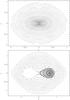 |
Fig. 1 Poincaré surfaces of section for the “exponential” potential with q = 0.8 and energies E = −0.5 (top) and −0.2 (down). |
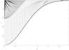 |
Fig. 2 Isolevels of x-axis orbit apocentres versus xinit and E. At low energies box orbits dominate the diagram. Tube orbits (type 1:1) become significantly present at E > −0.4. At E = −0.05, they cover the range xinit from 0 to 1.4. Higher order resonances draw visible “plumes”. |
3. Exponential potential
We apply the method described in Sect. 2 to obtain an approximate integral of motion to the case of the following barred potential: 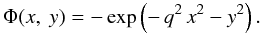 This potential is chosen for its simplicity: bounded orbits have energies in a limited range within [− 1, 0] and most orbits are regular. The density associated to the potential is not positive everywhere but the Taylor series of this potential has an infinite radius of convergence that should allow us, in a future work, an easier comparison of our results to formal integrals obtained by other means (Giorgilli & Galgani 1978).
Most of the bounded orbits (E < 0) are regular. They are box and tube orbits (libration and circulation), and most of the tube orbits are of type (1:1). This can be seen in Poincaré surfaces of section (Figs. 1) or with the 2D isolevel plot of x-apocentre (at u = y = 0) versus the energy and the initial position xinit (at u = y = 0) (Fig. 2). In this last figure, high-order resonances appear at the highest energies and draw inclined “plumes”.
To build the polynomial quasi integral of motion, we select orbits that cover a wide range of energies and a wide range of second constants of motion, taken as the orbit initial position xinit (u = y = 0) (in this example, we consider only orbits that cross the x-axis perpendicularly, which excludes very few orbits that appear mainly at high energies.)
We also select the polynomial terms used to determine I. Due to the x- and y-axis symmetries of the potential, the coefficients of terms in Eq. (1) with l + m or k + n odd are set to zero. The momenta parity of I is even (m + n even). We set the coefficient of x2 to one, remove all x2k (k > 1) and all v2l terms. The final series thus obtained will be independent of E and a unique solution for the coefficients is expected.
The remaining coefficients of the series in Eq. (1) are obtained by a least-squares minimisation, and the quality of the fit is quantitatively defined by the constancy of I along each orbit. The result of the fit critically depends on the existence or non-existence for the examined potential of an approximate integral that remains nearly constant over long periods of time along orbits. But the quality, also critically, depends as any polynomial fit, on a convenient coverage of the fitted space to adjust structures, and on a sufficiently large number of coefficients to model the numerous and small structures. Finally, it also depends on a sufficiently large number of fitted data to avoid or at least to minimise erratic oscillations between fitted data. For this, we impose that the number of fitted positions is sufficiently large by applying the recommended conditions that  (Dalquist & Björk 1974). We must also ensure a sufficient coverage: 1000 positions on each orbit corresponds to a mean distance of 11 deg for the angle positions, assuming the couple of angles and actions were known.
Orbits are computed with a fourth-order Runge-Kutta integrator, the time step is fixed and the energy is conserved at 10-8. The minimisation is written as a linear least-squares fit, inversion is performed using the LAPACK softwares and presents no peculiar difficulties, because the matrix size remains small.
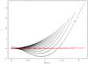 |
Fig. 3 Second integral of motion I (polynomial of order 12) versus xinit for 2085 orbits covering 19 energies. Orbits with the same energy draw 19 dotted lines. Box orbits have I > 0, tube orbits have I < 0. The red continuous line is the dispersion of I, it increases at resonances. |
3.1. Results
The first example is obtained with the following conditions: we select 2085 orbits covering energies E = −0.95, −0.9,..., −0.05 and at each energy with initial conditions (xinit, yinit = 0, uinit = 0, vinit(E,xinit)) xinit covering the interval 0 to xmax(E) by step Δxinit = 0.01. For each orbit, 1000 positions are taken (time step ΔT = 4) from T = 0 to 4000. After removing cancelled terms, we use the first 200 coefficients of Eq. (1), a 12th order polynomial, and after fitting, following the procedure described in the previous section, we obtain I12 a quasi invariant integral of motion.
We find that the mean value,  , varies from orbit to orbit between ~− 1 and ~+ 4.6 (Fig. 3) and that the mode (histogram maximum) of the dispersions σI12 along each orbit is 0.002, and σI remains within [5 × 10⁻⁴−3 × 10⁻³] for the low-energy orbits (E < −0.5). At higher energies, 30 orbits close to resonances have σI within [0.03−0.15] , the remaining 1360 orbits have σI smaller than 0.03 and a mode equal to 0.002.
We find that I12 remains nearly invariant over long periods by computing for each of the 2085 orbits over the time interval ΔT = 4 × 10⁶, corresponding approximately to 50 000 rotations, a much longer time than the interval ΔT = 4 × 10³ used for the fit (50 rotations). The variations of I12 (i.e. its residuals) are identical to a few percent to residuals obtained within the fitted time interval and, thus, we conclude that I12 can be extrapolated in time far outside the fitted domain (but of course not outside the fitted domain in coordinates and momenta).
We extend this check to examine the variation of I12 for orbits not used for the fit. Therefore, we explore in detail the energy-xinit fitted domain with a finer grid in energy (ΔE = 0.01 and Δxinit = 0.0025) using ~32 000 orbits. For these orbits the dispersion remains very close to the dispersion of the nearby orbits used for the fit. This confirms that we use a sufficiently large number of orbits and positions and that the interpolation between fitted orbits is correctly achieved.
Figure 3 presents, for each of the 2085 orbits, the mean value of I12 along the orbit versus its initial positions xinit. For each orbit, xinit is either its x-pericentre or its x-apocentre along the x-axis (thus with y = u = 0). Each dotted line represents a sequence of orbits with an identical value of the energy.
The two main families of orbits are box orbits and tube orbits (with type 1:1), corresponding to positive and negative values of I12. The family of box orbits is dominant at low energies, E ≲ −0.4. At all energies, the 1:1 periodic tube orbit corresponds to the minimum of I12. For most of the orbits, there is a one-to-one relation between each orbit and a couple of values (E,I). This useful property is lost, however, when the fit is improved to adjust higher order resonances, as we show below.
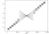 |
Fig. 4 For 19 orbits with E = −0.05 close to the resonance 2:3, I(t) is plotted every Δt = 4 over the time interval T = 4000. The dispersion of I(t) increases for orbits close to the resonance. The time sequence is shifted for each orbit for visibility. |
As a consequence of our specific choice of the cancelled coefficients within Eq. (1), we have I = 0 for the radial orbits aligned along the y-axis. On the other side, the x-axis radial orbits are, at a given energy, the orbit with the largest x-apocentre, Xsup,E, and we have I(Xsup,E,0,0,0) =  .
.
In Fig. 3, the dispersion σI12 is also plotted. This dispersion increases abruptly at the proximity of extended resonances. In Fig. 4, we plot I12(t) for 19 orbits close to a resonance 2:3 at E = −0.05. In this figure, for each orbit I12(t) is plotted every ΔT = 4 from T = 0 to 4000 (and each plotted orbit is shifted for better visibility). Crossing the resonance, the dispersion increases and is of the order of the variation of I, and within the resonance all orbits have approximately the same mean value for I12. As we show below, this can be improved by increasing the number of fitted positions on orbits to improve the sampling of the various tori of orbits, and by increasing the order of the fitting polynomial to allow the modelling of tori with smaller scale structures.
Semi-ergodic orbits are also present and are visible, confined between the tube and box orbits at E = −0.05 (Fig. 5). At energies E = −0.05, they correspond to orbits that pass close to the centre with xinit from 0 to ~0.07. Some of these orbits are included in the fit but do not alter the fitting quality: a possible cause is that they remain confined within a small volume and thus are reasonably adjusted as the immediately nearby regular orbits. The dispersion of I12 of the semi-ergodic orbits is significantly higher than for the nearby regular orbits, however.
Figure 5 (top-right) shows the Poincaré surface of section at E = −0.05 built from the fitted integral of motion I12. We note that only two families of orbits are identifiable because no high-order resonances are modelled.
3.2. Higher orders
To improve the approximate integral using the same data within the same time interval ΔT = 4000, we progressively increase the order of the fitted polynomial up to order 22 (2057 coefficients). By improving the fit, we mean that we reduce the variation of I within a given time interval ΔT. In contrast, we remark that formal forms of the second integral obtained also with polynomial series (Whittaker 1937; Birkhoff 1927; Contopoulos 1960; Gustavson 1966) lead to polynomial series that are asymptotic, i.e., up to an optimal order the accuracy of the series improves, and beyond this optimal order the accuracy decreases, the series being divergent. This is related to the Nekhoroshev (1977) theory (see also Contopoulos 2002, Sect. 2.3.6), which establishes that the formal integrals are valid over exponentially long (or short) times. Here, our approximate integral is different in the sense that it is always adjusted for a finite time interval, and its validity for longer time intervals has to be checked (the accuracy within the finite time interval can always be improved up to a certain limit L, and we expect that this limit L will increase when increasing the time interval, so that it does not contradict with the Nekhoroshev theorem). With the 2D potentials considered here, the long-term behaviour of the orbits can be constrained by absolute barriers in the phase space due to KAM tori (at the opposite of the case of higher dimensional potentials that allow Arnold diffusion). This may imply that our approximate integral variations would not increase for longer time. However, in the case of semi-ergodic orbits, orbits may be confined within a restricted domain of the phase space before reaching another domain if the domains are scarcely connected, as illustrated by Athanassoula et al. (1983, Fig. 8). In such cases we would expect that the integral variations increase for longer times.
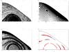 |
Fig. 5 Exponential potential, (x,u) Poincaré surfaces of section at E = −0.05 from the numerical and analytical I: (top-left) Numerical section, (top-right) analytical section obtained from a fit at order 12 and orbits at energies from −1 to −0.05, (bottom-left) from a fit at order 18 and orbits with energy E = −0.05, (bottom-right) from three local fits (order 18) of orbits in the neighbourhood of three resonant orbits, the empty space between the islands of stability is not filled correctly by the analytical integrals (red dots are the sections, y = 0 and v > 0, from computed orbits). |
Figure 6 shows the mean I and dispersion σI for each orbit, the values are presented sequentially by group of energy (left to right E varies from −0.95 to −0.05). Increasing the polynomial order allows us to model more resonances. At order 10 the only one minimum of I corresponds to the resonant orbit 1:1. At higher polynomial order, I has more extrema corresponding to secondary resonances. The dispersion through these resonances decreases progressively as the order of the polynomial increases: from order 12 to 20 the mode (histogram maximum) of σI changes from 0.050 to 0.0007, while the mean of σI varies from 0.18 to 0.011. The mean dispersion increases at order 22, but the highest values of σI at resonances decrease significantly.
We define a more quantitative criterion to consider the ability to distinguish two nearby orbits with the same energy: the relative dispersion as the ratio of the dispersion σI to the variation of I between orbits: 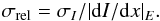 This relative dispersion has the dimension of x, here with values of a few 10-4 and can be compared to the full range of variations of x from 0 to about 2. This relative accuracy is the poorest at resonances when (dI/dx)E = 0, but the mode of σrel varies from 5. × 10-4 to 1.5 × 10⁻⁴ when the polynomial order changes from order 12 to 20. The mean σrel (clipped within [0 to 1. × 10-2]) decreases first but then flattens at 1.0 × 10⁻³ from the orders 14 to 20.
Increasing the polynomial order allows us to model more resonances. At low order from 8 to 16 only the two main families are modelled, as is visible in the reconstructed Poincaré section at E = −0.05 (Fig. 5). At orders 18 to 22 three more resonances are visible in the reconstructed Poincaré surface of section corresponding to families 2:3, 3:4, and 3:5. Only the family 2:3 (extended from x = 0, u = 1.06 to x = 1.9, u = 0) is accurately modelled, the two other ones are incorrectly positioned. Considering the small size of the structures of these resonances, we suspect that a higher order polynomial fit is necessary and also because increasing the polynomial order progressively improves the fit.
Owing to limited computing resources we did not explore this systematically with much higher polynomial orders. Nevertheless, we explored fits with a restriction to orbits just close to the energy E = −0.05 using 2200 orbits. The resulting fit is better (Fig. 5) with now two resonances correctly positioned within the surface of section, but only the family 2:3 has the correct multiplicity of islands. Now the family 3:4 is also correctly positioned, but the number of reconstructed islands is incorrect, but by increasing the polynomial order, the exceeding island progressively disappears.
Finally, we proceed to the local fit of the three resonances. Figure 5 shows the reconstructed Poincaré surface of section from the three analytical approximate integrals of motion that shows a satisfying fit. A second 1:4 family (not used for the fit) is also correctly modelled (the corresponding periodic orbit never cross the x-axis perpendicularly).
All these results point out that for this potential, an approximate integral is constant with a very high accuracy. There is also a strong indication that a better modelling of I could be achieved by using a polynomial of sufficiently high order.
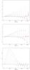 |
Fig. 6 Integral I for 2085 orbits covering 19 energies. From top to bottom, fits with polynomials of order 10,16 and 22. Orbits are plotted sequentially according to their initial position xinit, and according to the energy (E = −0.95 left to E = −0.05 right). The red line is the dispersion of I multiplied by 10. |
3.3. Other combination of coefficients
We have tried about 30 different combinations of coefficients to numerically build quasi integrals I: all with the same number of coefficients, and the fixed term is either x2, v2 or x2v2. The efficiency or accuracy of I is determined according to the value σrel for every orbit. The various combinations are not equivalent in terms of efficiency, some give a better fit for orbits with high energies, others for low energies. The four following combinations give the best results
-
coefficient of x 2 set to 1, all others v 2n and x 2k are zero,
-
coefficient of x 2 set to 1, all others y 2l and x 2k are zero. With these combinations we have

-
coefficient of v 2 set to 1, all other v 2n and x 2k are zero,
-
coefficient of v 2 set to 1, all other v 2n and u 2m are zero. With these combinations

4. Logarithmic potentials
To check that the numerical results described in the previous section have some generality, we considered other potentials. These potentials have a very limited amount of ergodicity, the chaotic orbits remaining confined within a small volume of the phase space. We also limited most of our fits using polynomials with order smaller than 18 to avoid prohibitively long computing times (100 h.cpu).
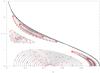 |
Fig. 7 Logarithmic potential: (x,u) Poincaré surface of section at E = 0 for three families of orbits (circles) and three different analytical tori (continuous lines) obtained with polynomials of order 18. |
4.1. Scale-free logarithmic potential
The logarithmic potential introduced by Richstone (1980) to model axisymmetric disc galaxies produces a flat rotation curve: 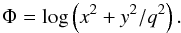 The parameter q allows us to model a flattening of the potential and of the corresponding density. The density is not positive everywhere when with
  , and that with
  the density isocontours present a depression close to the y-axis.
A detailed analysis of orbits in this potential was presented by Miralda-Escudé & Schwarzschild (1989) with plotted Poincaré surfaces of section. This potential has semi-ergodic motions (Papaphilippou & Laskar 1996) and is not integrable. Chaotic orbits have excursions close to the centre and circulate around the sets of tori of the major families of resonant orbits. The phase space is mainly occupied by regular orbits (at least with q from 0.2 to 1) and the dominant families of these regular orbits are tube orbits of type 1:1. Box orbits of type 2:1, 3:2, 4:3, etc. (also named boxlets orbits : banana, fish, pretzel, etc.) cover most of the remaining surface of the Poincaré section.
Using the procedure described in Sect. 2, we determined polynomial forms to evaluate a second integral of motion by fitting orbits of type 1:1, 2:1, and 3:2 (this is done only with E = 0 since the potential is scale-free and the integral can be simply deduced for other energies). Using polynomials of order 18, we succeeded in modelling most of the orbits of each of these three families separately. Thus, a different polynomial was used for each of the three families (Fig. 7). We also obtained a general fit of the three families with a unique polynomial of order 28 (4760 coefficients), but just two-thirds of the orbits plotted in Fig. 7 are fitted (the orbits close the central periodic orbits). Within the surface of section (x, u), these unfitted orbits are poorly fitted when x ≲ 0.1 but are correctly fitted at larger x.
The scale-free logarithmic potential is the one for which the application of our method gives the most limited success. As for the other potentials, we used our program to fit the energy E(x,y,u,v) considering it as a polynomial and consequently also the potential Φ(x,y). Not surprisingly, a polynomial form hardly fits a logarithmic function without core. Furthermore, examining the Boltzmann equation for this potential, we can assume that to build a second integral with a formal series, a series of rational functions will be more suited. Here, the Prendergast (1982) method to obtain rational solutions should be certainly more efficient.
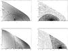 |
Fig. 8 Logarithmic potential with a core: (x,u) (top) and (y,v) (bottom) Poincaré surfaces of section at E = 3. Fits with an 18th order polynomial from orbits with E = 0 to 3.5. Computed orbits (right) and anaytical tori (left). |
4.2. Logarithmic potential with a core
As suggested by Richstone (1980) and already used by Binney (1981) and Magnenat (1982), the logarithmic potential  has a core. We examine this potential with a = 1 and q = 0.8. The presence of a core drastically reduces the extent of the semi-ergodic orbits for energies E < 4 (and a = 1). It is at much higher energies and with x or y coordinates much larger than the core radius a, that orbits are similar to the orbits within the logarithmic potential seen in Sect. 4.1. At low energies box orbits dominate, type 1:1 tube orbits appear at E ~ 0.9.
We obtain a good fit for orbits from E = 0 to 3 with a 12th order polynomial (and coefficients selected as in Sect. 3.1), the fit is good everywhere except close to the transition between box and tube orbits, the less accurately fitted region being at the apparition of tube orbits when E ~ 0.9. The fit is greatly improved, however, by increasing the number of orbits in this transition region, for instance using 23 428 orbits (1000 positions along each orbit) and order 16. Some resonant orbits are not modelled (see Fig. 8, (y,u) Poincaré section at E = 3.0, and (y,v) = (0.8, 0) or (0, 1.5) or (1.7, 1.5)) but they cover a very small volume of the phase space. Increasing the order to the 18th order, the fit improves, but high-order resonances are still poorly fitted. Fitting orbits from E = 0 to 3.5 (with 27 619 orbits) with 5000 positions on each orbit and order 18, the fit improves from E = 0 to 3.
4.3. Axisymmetric scale-free logarithmic potential
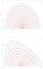 |
Fig. 9 Axisymmetric logarithmic potential: orbits with Lz = 1. (top to bottom): (x,u) Poincaré surface of section with E = 0.01 and .5. Computed orbits (dotted red circles) and analytical reconstructed tori (continuous dark lines) with an 18th order polynomial fitted along orbits with E = 0 to 0.5. |
Still following Richstone (1980), we consider a 3D flattened logarithmic potential and motions with non-null angular momentum. We set no core (a = 0) and a flattening parameter q = 0.8 and consider only orbits with the same angular momentum Lz = 1. Results for any other non-null Lz are easily deduced. Thus we consider orbits in the effective potential  Eeff close to zero corresponds to nearly circular obits around the z-axis. The radial orbits with z = 0 and a null vertical velocity dispersion σz are a first family of periodic orbits. The shell orbits with a null radial velocity vR when z = 0 are another family. For a given Eeff, the amount of radial versus vertical extension of an orbit is constrained by a second integral (see for instance Ollongren 1962). The rotation prevents orbits from circulating close to the centre and thus reduces the amount of ergodic orbits by comparison to the case with Lz = 0. Chaotic orbits occupy an extremely small volume in the phase space, at least for Eeff < 8. At low energies (E ≲ 1) orbits are mainly box orbits.
Radial orbits have z = 0 and at their two extrema Rmin and Rmax have also vR = vz = 0. Thus, for all such orbit: I(Rmin,0,0,0) = I(Rmin,0,0,0), a relation that can be achieved only if I(R,0,0,0) = f(Φ(R,z = 0)). The choice of coefficients in Sect. 3.1 does not allow us to fulfil this condition. Therefore here we set to one the coefficient of  and remove all
  , with n > 1, and all
  terms (removing all , with m > 1, and all R2k is also satisfying).
Figure 9 shows the results of a fit with 24 000 orbits (100 positions on each orbit) with E = 0 to 0.5, and an 18th order polynomial.
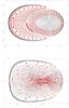 |
Fig. 10 Toda lattice: (top) (y,v) Poincaré section at (x = 0, u > 0) and E = 1/12 and analytical tori (continuous lines) with a 14th order polynomial. (Bottom) (y,v) Poincaré section at (x = 0, u > 0) and E = 1 for a few orbits (dotted red circles) and analytical tori (continuous dark lines) with a 16th order polynomial. |
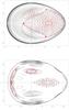 |
Fig. 11 Hénon & Heiles potential: (top) (y,v) Poincaré section at (x = 0 and u > 0) and E = 1/12 for a few orbits (dotted red circles) and analytical tori (continuous dark lines) with a 12th order polynomial. (Bottom) Poincaré section at E = 1/8 for a few regular orbits (dotted red circles) and analytical tori (continuous dark lines) with an 18th order polynomial, the unplotted domain is covered by chaotic orbits. |
5. Hénon & Heiles and Toda lattice potentials
We do not present the various tests of our procedure performed with integrable dynamical systems: axisymmetric, Stäckel potentials, or systems with a second integral with a finite polynomial form.
Instead, we summarise the results obtained for two classic potentials, the Toda (1970) lattice (2D case) and the Hénon & Heiles (1964) potential (a historical description concerning these potentials on simulations in dynamics is given by Weissert 1997). The Toda lattice potential has a known analytical second integral (Hénon 1974; Manakov 1974, 1975; Flaschka 1974). The Hénon & Heiles potential has regular orbits at low energies while nearly full ergodicity appears at high energies. The two potentials are closely linked since the first four terms of the series development of the 2D Toda lattice give the Hénon & Heiles potential, one is integrable, the other one shows a nearly complete dynamical chaos at high energies. The functional form of the second integral of the Toda lattice is known and is odd for the momenta reflecting that there is no box orbit but only circulating motions (tube orbits). The extrema of the second integral at fixed energy allows the precise identification of the family of stable orbits. This potential and its second integral can be written as a polynomial series with an infinite radius of convergence for all coordinates. This was assumed to be important as a first step to test the procedure developed in this paper, which assumes that a polynomial series exists to represent the hypothetic second integral.
5.1. Toda lattice
Selecting 79 orbits with energy E = 1/12, 10 000 positions on each orbit, and a fit at order 14, we obtain a median relative accuracy of 1.2 × 10⁻⁵. We obtain 7.5 × 10⁻⁷ at order 16 (Fig. 10). Selecting a uniform distribution of 1700 orbits from energy E = 0 to 1, still with 10 000 positions, we obtain a median relative accuracy of 1.5 × 10⁻¹ at order 14 and 3.5 × 10⁻² at order 18. We also succeed in obtaining a good fit from E = 0 to 4 with 2800 orbits. The polynomial expansion of the known Toda lattice second integral contains only terms of order 0, 1 or 3 in the momenta v. Our a priori construction and fit of a polynomial series does not impose such a constraint on the coefficients, accordingly our fitted series requires a much larger number of terms and coefficients to achieve the same accuracy as using the polynomial form of the known integral.
5.2. Hénon & Heiles potential
Within the Hénon & Heiles potential, we compute 10 000 positions along 41 orbits with the energy E = 1/12 (ΔT = 10 000). The recovered analytical tori are quantitatively correct and better than a few thousandths in relative accuracy at orders higher than the 7th (83 coefficients). Figure 11 may be compared to the result of Gustavson (1966, Fig. 13), where the integral of motion was determined by symbolically manipulating polynomials up to the order 7. At order 12, our median relative accuracy is improved: 2 × 10⁻⁴, and at order 14 it is 10-4.
At energy E = 1/8 an ergodic orbit covers about half of the phase space (see Fig. 5 in Hénon & Heiles 1964). We obtain a roughly approximate integral of motion for the regular orbits close to the main periodic orbits. With a fit of 54 regular orbits close to the resonance 1:1, the recovered analytical tori (Fig. 11) show that the three main families are recovered. This may be compared to the results of Gustavson (1966, Fig. 10) obtained at the same energy: he obtained analytical sections in good qualitative agreement with the sections plotted from computed orbits. More recent works (see Kaluza & Robnik 1992; Robnik 1993; Contopoulos et al. 2003) give higher orders of formal integrals and show a better agreement at energy E = 1/8 where the chaotic orbits occupy a large volume of the phase space.
6. Conclusion
Obtaining integrals of motion of a dynamical system simplifies the analysis and the understanding of the system, because it allows us for instance to build more easily tractable distribution functions. It also gives a synthetic description of the orbits, the building blocks of galaxies. This is well-known for axisymmetric systems, and it has been also extensively developed for Stäckel potentials. Other systems with known analytic integrals are apparently less interesting for the astronomical community.
Therefore many efforts and methods have been developed to obtain approximate integrals of motions for more general potentials. Moser’s theorem states that most invariant curves will be preserved under a weak perturbation of an integrable dynamical system. A method initiated by Birkhoff (1927) consists of writing the Hamiltonian in the so-called normal form, which allows the formal construction of polynomial series that are solutions of the Boltzmann equation.These series are generally divergent (Siegel 1941; Contopoulos et al. 2003). Even for an integrable system, they may be not convergent (Wood & Ali 1987). Gustavson (1966) developed an algorithm to obtain these formal integrals and applied it to the Hénon & Heyles potential.
A more direct method by Whittaker (1937) or Contopoulos (1960) also consisted of looking for formal polynomial integrals of motion, but did this directly by substituting and comparing coefficients. Giorgilli & Galgani (1978) solved the consistency problem of these direct methods.
Inspired by these methods, Giorgilli & Galgani (1978) proposed a new method for constructing formal integrals near an equilibrium point, and a numerical program (Giorgilli 1979) was used for applications (see for instance Kaluza & Robnik 1992; Contopoulos et al. 2003). The formal integrals are different for resonant and each non-resonant orbit (Contopoulos et al. 2000).
A different technique, called torus construction (for a review, see Valluri & Merritt 1999), consists of numerically mapping the action-angle coordinates of a known potential into the action-angle coordinates for the system under investigation (McGill & Binney 1990). This is obtained by a least-squares procedure. It implies the availability of a close and integrable Hamiltonian whose tori can be simply mapped to the target tori; it also implies mappings from different toy tori for different orbit families (Kaasalainen & Binney 1994). Moreover, there are general methods of semi-numerical perturbation that take into account the full “distortion” of the invariant tori (Henrard 1990).
The method developed in this paper partly builds on previously published methods. We solved the Boltzmann equation with a polynomial, but numerically and with a fit to many peculiar solutions (i.e. orbits). This method is a priorilimited by the accuracy with which the invariant curves are defined on the surfaces of section, i.e. to which point they are effectively invariant and affected by diffusion. This limiting accuracy depends, for a given potential and a given orbit, on the time interval of integration of the orbit. But for a given time interval, it should be sufficient to increase the order of the fitting polynomial to achieve higher accuracy. We succeeded in different examples to fit various resonant and non-resonant families of orbits with the same integral. The quality of the fits depends on selected coefficients of a polynomial series. Here, the method was applied to various 2D potentials representative of motions within elliptical galaxies or motions within a non-axisymmetric disc. For all these potentials, a unique analytical integral of motion was obtained for an extended range of energies and regular orbits. The coefficients of the polynomial of the integrals were obtained from a linear least-squares minimisation. Warnock (1991) and Bazzani et al. (1991) also developed methods of orbit fitting but with limitations; the former with restrictions to high-order resonant orbits or non-resonant orbits, the latter to 2D sections. In addition, they did not impose the energy independence of their integral, which may impact the numerical accuracy of the fitted second integral.
As a future development, the method presented in this paper will be applied to the construction of a simple 3D galactic model. We will use a scale-free logarithmic disc-halo potential (Bienaymé 2009), for which a third integral I3 will be determined: the third integral is first determined for a given value of the energy and a given non-zero angular momentum, and is then simply deduced for other values of E and Lz. Afterwards, the action can be evaluated from I3. Finally, a distribution function for an exponential stellar disc can be built following the generalisation of the Shu distribution function by Kuijken & Dubinski (1995), Bienaymé & Séchaud (1997), or Bienaymé (1999). This model will allow us to explore various properties: for instance, to check the domain of validity of the asymmetric drift relation especially out of the mid-plane, to examine the velocity ellipsoid tilt dependence on the distribution function, or to build a realistic model to measure the Kz force from data far above and below the galactic plane by minimising the number of free parameters and assumptions in the modelling.
Stäckel potentials, as they are called in the astronomical literature, are usualy named Darboux potentials in the mathematics literature. A first systematic attempt to study quadratic invariants is given in Darboux (1901). Contributions on separability, orthogonal coordinate systems, and quadratic invariants may be found in Ankiewicz & Pask (1983).
Here, we do not answer the question of the convergence of these iterative operations. Our success in obtaining approximate integrals in the next paragraphs indicates that the iterations can build at least asymptotic series.
References
- Ankiewicz, A., & Pask, C. 1983, J. Phys. A Math. General, 16, 4203 [NASA ADS] [CrossRef] [Google Scholar]
- Athanassoula, E., Bienaymé, O., Martinet, L., & Pfenniger, D. 1983, A&A, 127, 349 [NASA ADS] [Google Scholar]
- Bazzani, A., Remiddi, E., & Turchetti, G. 1991, J. Phys. A Math. General, 24, 53 [NASA ADS] [CrossRef] [Google Scholar]
- Bienaymé, O. 1999, A&A, 341, 86 [NASA ADS] [Google Scholar]
- Bienaymé, O. 2009, A&A, 500, 781 [NASA ADS] [CrossRef] [EDP Sciences] [Google Scholar]
- Bienaymé, O., & Séchaud, N. 1997, A&A, 323, 781 [NASA ADS] [Google Scholar]
- Binney, J. 1981, MNRAS, 196, 455 [NASA ADS] [Google Scholar]
- Binney, J., & Kumar, S. 1993, MNRAS, 261, 584 [NASA ADS] [Google Scholar]
- Binney, J., & Spergel, D. 1982, ApJ, 252, 308 [NASA ADS] [CrossRef] [Google Scholar]
- Birkhoff, G. 1927, Dynamical systems American Math Soc., New York, IX [Google Scholar]
- Contopoulos, G. 1960, ZAp, 49, 273 [Google Scholar]
- Contopoulos, G. 2002, Order and chaos in dynamical astronomy (Springer, Astronomy and astrophys library) [Google Scholar]
- Contopoulos, G., Efthymiopoulos, C., & Voglis, N. 2000, Celest. Mecha. Dyn. Astron., 78, 243 [Google Scholar]
- Contopoulos, G., Efthymiopoulos, C., & Giorgilli, A. 2003, J. Phys. A Math. General, 36, 8639 [Google Scholar]
- Dalquist, G., & Björk, A. 1974, Numerical Methods (ed. Prentice-Hall) [Google Scholar]
- Darboux, G. 1901, Archives Néerlandaises, 6, 371 [Google Scholar]
- Efthymiopoulos, C., Voglis, N., & Kalapotharakos, C. 2007, in Lect. Not. Phys., eds. D. Benest, C. Froeschle, & E. Lega (Berlin: Springer Verlag), 729, 297 [NASA ADS] [Google Scholar]
- Flaschka, H. 1974, Phys. Rev. B, 9, 1924 [NASA ADS] [CrossRef] [Google Scholar]
- Giorgilli, A. 1979, Comput. Phys. Comm., 16, 331 [Google Scholar]
- Giorgilli, A., & Galgani, L. 1978, Celest. Mecha., 17, 267 [Google Scholar]
- Gustavson, F. G. 1966, AJ, 71, 670 [NASA ADS] [CrossRef] [Google Scholar]
- Hénon, M. 1974, Phys. Rev. B, 9, 1921 [NASA ADS] [CrossRef] [Google Scholar]
- Hénon, M. 1983, in Chaotic behaviour of deterministic systems, eds. G. Ioss, R. Helleman, & R. Stora (North-Holland publishing company), 53 [Google Scholar]
- Hénon, M., & Heiles, C. 1964, AJ, 69, 73 [NASA ADS] [CrossRef] [Google Scholar]
- Henrard, J. 1990, Celest. Mecha. Dyn. Astron., 49, 43 [Google Scholar]
- Hietarinta, J. 1987, Phys. D Nonlinear Phenomena, 28, 248 [Google Scholar]
- Kaasalainen, M. 1994, MNRAS, 268, 1041 [NASA ADS] [Google Scholar]
- Kaasalainen, M. 1995, MNRAS, 275, 162 [NASA ADS] [Google Scholar]
- Kaasalainen, M., & Binney, J. 1994, MNRAS, 268, 1033 [NASA ADS] [Google Scholar]
- Kaluza, M., & Robnik, M. 1992, J. Phys. A Math. General, 25, 5311 [NASA ADS] [CrossRef] [Google Scholar]
- Kuijken, K., & Dubinski, J. 1995, MNRAS, 277, 1341 [CrossRef] [Google Scholar]
- Laskar, J. 1993, Celest. Mecha. Dyn. Astron., 56, 191 [Google Scholar]
- Magnenat, P. 1982, A&A, 108, 89 [NASA ADS] [Google Scholar]
- Manakov, S. V. 1974, Soviet J. Exp. Theoret. Phys., 40, 269 [NASA ADS] [Google Scholar]
- Manakov, S. V. 1975, Z. Eksper. noi Teoretich. Fiz., 67, 543 [NASA ADS] [Google Scholar]
- McGill, C., & Binney, J. 1990, MNRAS, 244, 634 [NASA ADS] [Google Scholar]
- Miralda-Escudé, J., & Schwarzschild, M. 1989, ApJ, 339, 752 [NASA ADS] [CrossRef] [Google Scholar]
- Morbidelli, A., & Giorgilli, A. 1995a, Phys. D Nonlinear Phenomena, 86, 514 [NASA ADS] [CrossRef] [Google Scholar]
- Morbidelli, A., & Giorgilli, A. 1995b, J. Statist. Phys., 78, 1607 [NASA ADS] [CrossRef] [Google Scholar]
- Nekhoroshev, N. N. 1977, Russian Mathematical Surveys, 32, 1 [Google Scholar]
- Ollongren, A. 1962, Bull. Astron. Inst. Netherlands, 16, 241 [Google Scholar]
- Papaphilippou, Y., & Laskar, J. 1996, A&A, 307, 427 [NASA ADS] [Google Scholar]
- Prendergast, K. 1982, in The Riemann Problem, eds. D. Chudnowsky, & G. Chudnowsky (Springer-Verlag) [Google Scholar]
- Richstone, D. O. 1980, ApJ, 238, 103 [NASA ADS] [CrossRef] [Google Scholar]
- Robnik, M. 1993, J. Phys. A Math. General, 26, 7427 [NASA ADS] [CrossRef] [Google Scholar]
- Schwarzschild, M. 1979, ApJ, 232, 236 [NASA ADS] [CrossRef] [Google Scholar]
- Siegel, C. 1941, Ann. Math., 42, 806 [CrossRef] [Google Scholar]
- Stäckel, P. 1893, Math. Ann., 42, 548 [CrossRef] [Google Scholar]
- Syer, D., & Tremaine, S. 1996, MNRAS, 282, 223 [NASA ADS] [CrossRef] [Google Scholar]
- Toda, M. 1970, Prog. Theor. Phys. Suppl., 45, 174 [NASA ADS] [CrossRef] [Google Scholar]
- Valluri, M. & Merritt, D. 1999, in Galaxy Dynamics – A Rutgers Symposium, eds. D. R. Merritt, M. Valluri, & J. A. Sellwood, ASP Conf. Ser., 182, 178 [Google Scholar]
- Valluri, M., Debattista, V. P., Quinn, T. R., Roškar, R., & Wadsley, J. 2012, MNRAS, 419, 1951 [NASA ADS] [CrossRef] [Google Scholar]
- Warnock, R. L. 1991, Phys. Rev. Lett., 66, 1803 [NASA ADS] [CrossRef] [Google Scholar]
- Weissert, T. 1997, The Genesis of Simulation in Dynamics (Springer) [Google Scholar]
- Whittaker, E. 1937, A Treatise on the Analytical Dynamics of Particles and Rigid Bodies (Cambridge University Press) [Google Scholar]
- Wood, W. R., & Ali, M. K. 1987, J. Phys. A Math. General, 20, 351 [NASA ADS] [CrossRef] [Google Scholar]
All Figures
|
Fig. 1 Poincaré surfaces of section for the “exponential” potential with q = 0.8 and energies E = −0.5 (top) and −0.2 (down). |
| In the text | |
|
Fig. 2 Isolevels of x-axis orbit apocentres versus xinit and E. At low energies box orbits dominate the diagram. Tube orbits (type 1:1) become significantly present at E > −0.4. At E = −0.05, they cover the range xinit from 0 to 1.4. Higher order resonances draw visible “plumes”. |
| In the text | |
|
Fig. 3 Second integral of motion I (polynomial of order 12) versus xinit for 2085 orbits covering 19 energies. Orbits with the same energy draw 19 dotted lines. Box orbits have I > 0, tube orbits have I < 0. The red continuous line is the dispersion of I, it increases at resonances. |
| In the text | |
|
Fig. 4 For 19 orbits with E = −0.05 close to the resonance 2:3, I(t) is plotted every Δt = 4 over the time interval T = 4000. The dispersion of I(t) increases for orbits close to the resonance. The time sequence is shifted for each orbit for visibility. |
| In the text | |
|
Fig. 5 Exponential potential, (x,u) Poincaré surfaces of section at E = −0.05 from the numerical and analytical I: (top-left) Numerical section, (top-right) analytical section obtained from a fit at order 12 and orbits at energies from −1 to −0.05, (bottom-left) from a fit at order 18 and orbits with energy E = −0.05, (bottom-right) from three local fits (order 18) of orbits in the neighbourhood of three resonant orbits, the empty space between the islands of stability is not filled correctly by the analytical integrals (red dots are the sections, y = 0 and v > 0, from computed orbits). |
| In the text | |
|
Fig. 6 Integral I for 2085 orbits covering 19 energies. From top to bottom, fits with polynomials of order 10,16 and 22. Orbits are plotted sequentially according to their initial position xinit, and according to the energy (E = −0.95 left to E = −0.05 right). The red line is the dispersion of I multiplied by 10. |
| In the text | |
|
Fig. 7 Logarithmic potential: (x,u) Poincaré surface of section at E = 0 for three families of orbits (circles) and three different analytical tori (continuous lines) obtained with polynomials of order 18. |
| In the text | |
|
Fig. 8 Logarithmic potential with a core: (x,u) (top) and (y,v) (bottom) Poincaré surfaces of section at E = 3. Fits with an 18th order polynomial from orbits with E = 0 to 3.5. Computed orbits (right) and anaytical tori (left). |
| In the text | |
|
Fig. 9 Axisymmetric logarithmic potential: orbits with Lz = 1. (top to bottom): (x,u) Poincaré surface of section with E = 0.01 and .5. Computed orbits (dotted red circles) and analytical reconstructed tori (continuous dark lines) with an 18th order polynomial fitted along orbits with E = 0 to 0.5. |
| In the text | |
|
Fig. 10 Toda lattice: (top) (y,v) Poincaré section at (x = 0, u > 0) and E = 1/12 and analytical tori (continuous lines) with a 14th order polynomial. (Bottom) (y,v) Poincaré section at (x = 0, u > 0) and E = 1 for a few orbits (dotted red circles) and analytical tori (continuous dark lines) with a 16th order polynomial. |
| In the text | |
|
Fig. 11 Hénon & Heiles potential: (top) (y,v) Poincaré section at (x = 0 and u > 0) and E = 1/12 for a few orbits (dotted red circles) and analytical tori (continuous dark lines) with a 12th order polynomial. (Bottom) Poincaré section at E = 1/8 for a few regular orbits (dotted red circles) and analytical tori (continuous dark lines) with an 18th order polynomial, the unplotted domain is covered by chaotic orbits. |
| In the text | |
Current usage metrics show cumulative count of Article Views (full-text article views including HTML views, PDF and ePub downloads, according to the available data) and Abstracts Views on Vision4Press platform.
Data correspond to usage on the plateform after 2015. The current usage metrics is available 48-96 hours after online publication and is updated daily on week days.
Initial download of the metrics may take a while.