© ESO, 2012

1. Introduction

Turbulence is thought to be a major actor throughout the lifetime of protoplanetary disks by regulating the mass accretion and angular momentum transport, planetesimal formation and planet migration, and mixing processes relevant for gas and grain chemistry (see, e.g. Henning 2008). The magneto-rotational instability (MRI, Balbus & Hawley 1991) is currently the most widely accepted theory for an origin of the effective turbulent viscosity. The ionization fraction in the outer disk is sufficient to allow for MRI to operate, but there may be a “dead” laminar zone in the inner (<10 AU) disk interior, efficiently shielded from ionizing radiation (Gammie 1996). Its extent depends on a variety of factors including magnetic field morphology, X-ray activity, abundance of metals, and dust properties (Ilgner & Nelson 2006). The 2D disk models by Keller & Gail (2004) and Tscharnuter & Gail (2007) show the possible presence of large-scale circulation (Urpin 1984; Regev & Gitelman 2002), but such motions would be suppressed by turbulence on the scale of the disk thickness. These meridional flows may be artifacts of the 2D-hydrodynamical disk models with fixed α viscosity. More realistic 3D MHD simulations do not show preferential directions of the large-scale gas-flows (see e.g., Flock et al. 2011)

Turbulence may also provide a source of relative velocities for grain coagulation to occur (e.g. Voelk et al. 1980; Beckwith et al. 2000). The interplay between gas and solid particle motion, would also lead to high local “dust” overdensities and planetesimal formation by gravitational collapse (Johansen et al. 2007, 2011). The turbulent state may have a strong impact on the migration efficiency (Papaloizou & Terquem 2006; Oishi et al. 2007; Uribe et al. 2011). Finally, models of gas-phase chemistry including surface chemistry on grains are sensitive to the level of turbulent mixing (e.g. Ilgner et al. 2004; Ilgner & Nelson 2006; Semenov & Wiebe 2011) which may partially explain the presence of cold CO in disks (Dartois et al. 2003; Semenov et al. 2006; Aikawa 2007; Hersant et al. 2009).

Despite this enormous importance of turbulence for disks, even its magnitude is poorly constrained. Most constraints on the anomalous viscosity parameter α come from measured accretion rates onto the star, which is mostly determined by inner disk properties. Hueso & Guillot (2005) have attempted to constrain the overall value of the α parameter by simulations of the viscous evolution of disks as a function of time. More recent results on viscous spreading of dust disks from Guilloteau et al. (2011) suggest α decreases with time, with values less than 0.001 near 100 AU after a few Myr.

Direct measurements of the nonthermal gas motions resulting from mesoscopic scale turbulence remain rare. Carr et al. (2004) report supersonic turbulence from CO overtone bands, but lower linewidths for H₂O in SVS13, suggesting strong turbulence in the upper layers of the inner disk. On the other hand, for the outer disk of DM Tau, Dartois et al. (2003) find marginally larger local velocity dispersion in ¹³CO than in ¹²CO, suggesting lower levels of turbulence in the upper layers than in the disk plane. The derived broadening, 0.07 to 0.14 km s^-1, is subsonic, but its exact value is difficult to assess because of the contribution of the thermal component. Piétu et al. (2007) find similar results for MWC 480 and LkCa 15. More recently, Hughes et al. (2011) have obtained a low value for TW Hya ( < 0.04 km s^-1), but up to 0.3 km s^-1 for the Herbig Ae star HD 163296 from CO J = 3–2 observations.

However, although ¹²CO is an interesting indicator, because of the significant opacities of the lower lying transitions, it only probes a thin upper layer in the disk, where strong temperature gradients may affect the apparent linewidth. To build a complete picture of turbulence in disks, it is thus essential to constrain the turbulence from other (optically thinner) tracers. CO isotopologues and other molecules like HCO⁺ and CN yield typical linewidths around 0.18 km s^-1 at 300 AU, but attributing this to thermal or nonthermal motions remains difficult, as their thermal width at 30 K is 0.14 km s^-1 (Piétu et al. 2007; Chapillon et al. 2012b). Moreover, current chemical models fail to explain their vertical location in the molecular layer since CN, CCH or HCN appear to be in a colder molecular layer than predicted (Henning et al. 2010; Chapillon et al. 2012b).

It is then important to reduce the uncertainty (and possible bias) introduced by the thermal contribution to the linewidth. Among molecules detected in disks, only CS is both abundant enough and sufficiently heavier than the previously cited ones.

We report here on the study of the CS molecule in the DM Tau disk. Observations are presented in Sect. 2, disk properties are derived in Sect. 3, and we discuss the results in Sect. 4.

2. Observations

Observations were carried out with the IRAM Plateau de Bure interferometer. We observed two different transitions of CS, the J = 3–2 line at 146.969047 GHz and the J = 5–4 line at 244.935609 GHz.

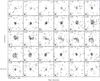Fig. 1 Channel maps of the CS J = 3–2 emission towards DM Tau. The angular resolution is 1.4′′ × 1.0′′ and the spectral resolution 0.16 km s-1. Contour spacing is 10 mJy/beam, corresponding to 2σ and 0.4 K brightness. The cross indicates the position, orientation, and aspect ratio of the dust disk.

For the J = 3–2 transition, we used the BC configuration (project RB8F). The B configuration, with baselines up to 408 m was observed on 18 Mar. 2008, while the more compact C configuration was observed on 15 Nov. 2008. Phase noise ranged from 15° up to 55° on the longest baselines. Amplitude calibration was done using nearby quasars and led to an rms level of about 5%. Absolute flux calibration was done using MWC 349 as a reference. The angular resolution is 1.4′′    × 1.0′′. The correlator provides only a limited spectral resolution with a channel spacing of 0.08 km s^-1, but with an effective resolution of 1.59 times the channel spacing (i.e. 0.126 km s^-1) owing to Welch apodization of the Fourier spectrum. At this resolution, the brightness sensitivity is 8.8 mJy/beam, which corresponds to 0.35 K at this angular resolution. Channel maps of CS(3–2) obtained after smoothing in velocity to 0.16 km s^-1 are presented in Fig. 1, but our analysis uses the unsmoothed data.

The CS(5–4) data were obtained on 11 Nov. 2004, 17 Nov. 2004, and 03 Apr. 2005 (Project OA45). The natural weighting spatial resolution is 2.6′′ × 1.8′′ at PA 85°. We smoothed the data to a spectral resolution of 0.25 km s^-1 for the analysis. The brightness sensitivity is 90 mJy/beam, corresponding to 0.4 K. The CS(5–4) is barely detected (at the 5σ level): a spectrum towards DM Tau obtained at 3.5′′ resolution is shown in Fig. 2. The data is compatible with the integrated spectrum obtained with the 30-m by Dutrey et al. (1997) and a source size of about 5′′, with an integrated line flux  ≃ 0.6 ± 0.1 Jy km s^-1.

The relative calibration accuracy between the two frequencies is better than 10%. It is based on the precise spectral index of 0.6 for the reference flux calibration source MWC 349.

3. Results

3.1. Principle of the method

Line formation in a Keplerian disk is strongly constrained by the velocity gradient (see, e.g. Horne & Marsh 1986, in the context of cataclysmic binaries). The line of sight velocity (in the system rest frame) is ${\mathit{V}}_{\mathrm{obs}}\mathrm{\left(}\mathit{r,\theta }\mathrm{\right)}\mathrm{=}\sqrt{\mathit{G}{\mathit{M}}_{\mathrm{\ast }}\mathit{/}\mathit{r}}\sin \mathit{i}\cos \mathit{\theta }$(1)where r,θ are the cylindrical coordinates in the disk plane. The locii of isovelocity are given by $\begin{array}{ccc}\mathit{r}\mathrm{\left(}\mathit{\theta }\mathrm{\right)}& \mathrm{=}& \mathrm{(}\mathit{G}{\mathit{M}}_{\mathrm{\ast }}\mathit{/}{{\mathit{V}}_{\mathrm{obs}}^{\mathrm{2}}}^{\mathrm{)}}{\sin }^{\mathrm{2}}\mathit{i}{\cos }^{\mathrm{2}}\mathit{\theta }\mathit{.}\end{array}$(2)With a finite local linewidth Δv (assuming rectangular line shape for simplification), the line at a given velocity V_obs originates in a region included between r_i(θ) and r_s(θ) : $\begin{array}{ccc}{\mathit{r}}_{\mathit{i}}\mathrm{\left(}\mathit{\theta }\mathrm{\right)}& \mathrm{=}& \frac{\mathit{G}{\mathit{M}}_{\mathrm{\ast }}}{\mathrm{(}{\mathit{V}}_{\mathrm{obs}}\mathrm{+}\mathrm{\Delta }\mathit{v}\mathit{/}\mathrm{2}{\mathrm{)}}^{\mathrm{2}}}{\sin }^{\mathrm{2}}\mathit{i}{\cos }^{\mathrm{2}}\mathit{\theta }\\ {\mathit{r}}_{\mathit{s}}\mathrm{\left(}\mathit{\theta }\mathrm{\right)}& \mathrm{=}& \begin{array}{}\min \end{array}\left[{\mathit{R}}_{\mathrm{out}}\mathit{,}\frac{\mathit{G}{\mathit{M}}_{\mathrm{\ast }}}{\mathrm{(}{\mathit{V}}_{\mathrm{obs}}\mathrm{-}\mathrm{\Delta }\mathit{v}\mathit{/}\mathrm{2}{\mathrm{)}}^{\mathrm{2}}}{\sin }^{\mathrm{2}}\mathit{i}{\cos }^{\mathrm{2}}\mathit{\theta }\right]\mathrm{·}\end{array}$Figure 3 indicates the regions of equal projected velocities for six different values: V_obs > v_d, V_obs = v_d, V_obs < v_d, and their symmetric counterpart at negative velocities, where v_d$\begin{array}{ccc}{\mathit{v}}_{\mathrm{d}}& \mathrm{=}& \end{array}$(5)is the projected velocity at the outer disk radius R_out. Figure 3 and Eq. (5) thus show that the basic shape of the emission as a function of velocity depends only on inclination i, while the stellar mass gives the scaling factor for the velocity scale. The intensity along the curves given by Eq. (5) will depend on the surface density Σ(r) and temperature T(r) profiles. On the other hand, the spatial spread perpendicular to this nominal shape depends only on the intrinsic linewidth Δv. With sufficient angular resolution, we thus expect that Δv is only very weakly coupled to any of the other disk parameters. The angular resolution should be at least high enough to measure the shape described by Eq. (5), i.e., measure the inclination i. A more stringent requirement is to resolve the transverse size perpendicular to the iso-velocity curves. An insufficient resolution would introduce a coupling between Δv and Σ or T as a smaller spatial spread can be compensated for by higher temperature (or opacity) to lead to the same flux density.

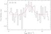Fig. 2 Spectrum of CS J = 5–4 line towards DM Tau. The angular resolution is 3.5′′ and the spectral resolution 0.25 km s-1. The curve is a best-fit Gaussian to emphasize the detection.

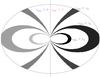Fig. 3 Regions of the disk that yield equal projected velocities vobs. The ellipse is the projection of the disk’s outer edge.

3.2. Simple model

To derive quantitative information from the data, we used the radiative transfer code adapted to disk DISKFIT (see Piétu et al. 2007, for a detailed description). In a first step (Model A), the CS column densities and rotational excitation temperature distributions are parameterized using a power law of the radius: 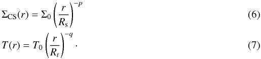$\begin{array}{ccc}& & {\mathrm{\Sigma }}_{\mathrm{CS}}\mathrm{\left(}\mathit{r}\mathrm{\right)}\mathrm{=}{\mathrm{\Sigma }}_{\mathrm{0}}{\left(\frac{\mathit{r}}{{\mathit{R}}_{\mathrm{s}}}\right)}^{\mathrm{-}\mathit{p}}\\ & & \mathit{T}\mathrm{\left(}\mathit{r}\mathrm{\right)}\mathrm{=}{\mathit{T}}_{\mathrm{0}}{\left(\frac{\mathit{r}}{{\mathit{R}}_{\mathit{t}}}\right)}^{\mathrm{-}\mathit{q}}\mathrm{·}\end{array}$\arraycolsep1.75ptAs explained by Piétu et al. (2007), T(r) is the line excitation temperature, and it is assumed to apply to all other levels to derive Σ(r). We further assume LTE, so that T(r) is now also the kinetic temperature. Then, the local linewidth consists of a thermal component, plus a turbulent contribution $\mathrm{\Delta }\mathit{V}\mathrm{\left(}\mathit{r}\mathrm{\right)}\mathrm{=}\sqrt{\frac{\mathrm{2}\mathit{kT}\mathrm{\left(}\mathit{r}\mathrm{\right)}}{\mathit{\mu }{\mathit{m}}_{\mathrm{H}}}\mathrm{+}\mathit{\delta }{\mathit{V}}_{\mathrm{tu}}\mathrm{(}\mathit{r}{\mathrm{)}}^{\mathrm{2}}}$(8)where μ = 44 is the CS molecular weight and m_H the atomic mass unit. We note that ΔV(r) is a half width at 1/e and that the full width at half maximum would be 1.66 times larger. The turbulent component is also parameterized by a power law $\mathit{\delta }{\mathit{V}}_{\mathrm{tu}}\mathrm{\left(}\mathit{r}\mathrm{\right)}\mathrm{=}\mathrm{d}{\mathit{V}}_{\mathrm{0}}{\left(\frac{\mathit{r}}{{\mathit{R}}_{\mathrm{v}}}\right)}^{\mathrm{-}{\mathit{e}}_{\mathit{v}}}\mathrm{·}$(9)Finally, CS is assumed to be homogeneously distributed in the z direction, with a scale height given by the disk midplane temperature. The density is given by ${\mathit{n}}_{\mathrm{CS}}\mathrm{=}\frac{{\mathrm{\Sigma }}_{\mathrm{CS}}}{\sqrt{\mathit{\pi }}\mathit{H}\mathrm{\left(}\mathit{r}\mathrm{\right)}}\exp \mathrm{(}\mathrm{-}\mathrm{(}\mathit{z}\mathit{/}\mathit{H}\mathrm{\left(}\mathit{r}\mathrm{\right)}{\mathrm{)}}^{\mathrm{2}}\mathrm{)}$(10)and the scale height is set to $\mathit{H}\mathrm{\left(}\mathit{r}\mathrm{\right)}\mathrm{=}{\mathit{H}}_{\mathrm{0}}\mathrm{(}\mathit{r}\mathit{/}{\mathit{R}}_{\mathit{h}}{\mathrm{)}}^{\mathrm{1.25}}$(11)with H₀ = 16 AU at R_h = 100 AU. This definition leads to a scale height that is $\sqrt{\mathrm{2}}$ times larger than the H(r) = c_s/Ω_K convention, where c_s is the sound speed and Ω_K the Keplerian angular velocity.

All the other geometric disk parameters (systemic velocity, inclination and position angle of the disk axis) were taken from the analysis of the CO isotopologues performed by Piétu et al. (2007). We also checked that CS gave consistent results with these independent measurements and that the errorbars on these geometric parameters did not affect the other derived parameters. A summary of the disk characteristics is given in Table 1.

Synthetic images are generated using the radiative transfer code DISKFIT, and model visibilities computed for each of the observed u,v points. Minimization on the disk free parameters is then made using a χ² criterion based on the difference between the observed and simulated visibilities. This process avoids the nonlinearities that result from deconvolution. A modified Levenberg-Marquardt method is used to locate the minima, with multiple restarts to avoid secondary minima. The linewidths we are searching for are not very large compared to the effective correlator resolution (0.126 km s^-1, see Sect. 2). Thus, we simulated the correlator spectral response by oversampling by a factor 4 in velocity space, i.e., using a velocity sampling bin of 0.02 km s^-1, followed by a convolution with a kernel mimicking the Welch apodization. This kernel extended over 12 consecutive channels in the oversampled frequency space.

Under these assumptions, the CS(3–2) line emission can be used to constrain Σ₀,p,T₀,q,dV₀ and e_v. Errobars around the minimum are derived from the covariance matrix. A proper choice of the pivot values R_t,R_v,R_s must be made to minimize the errors on the power laws (see Piétu et al. 2007, for details). With our angular resolution and CS images, R_t = R_v = R_s = 300 AU is a good compromise. A degeneracy occurs between Σ₀ and T₀ if the line is optically thin (for example, in the high temperature limit, the emission only depends on Σ₀/T₀), but this degeneracy is broken if the surface density profile is steep enough to produce an optically thick core (see Dutrey et al. 2007). Indeed, from a global fit, we find T(r) = (7.2 ± 0.4)(r/300   AU) ^{− 0.63 ± 0.09}   K. Assuming this temperature to be the kinetic temperature, we find an intrinsic nonthermal half width at 1/e, δV_tu(r) = 0.13 ± 0.03(r/300   AU) ^{− 0.38 ± 0.45} km s^-1. The outer radius is found to be 540 ± 10 AU.

The derived excitation temperature is unlikely to differ much from the kinetic temperature, because the densities in the disks are substantially higher than the CS(3–2) critical densities, even at the outer radius. To explain the observed total intrinsic width by thermal motions ($\mathit{\delta }{\mathit{V}}_{\mathrm{th}}\mathrm{=}\sqrt{\mathrm{2}\mathit{kT}\mathrm{\left(}\mathit{r}\mathrm{\right)}\mathit{/}{\mathit{\mu }}_{\mathrm{CS}}{\mathit{m}}_{\mathrm{H}}}$, with μ_CS = 44) would require a high value of T ≃ 50 K at 300 AU. This simple analysis thus indicates that pure thermal motions cannot reproduce the observed emission pattern, under the assumptions of Model A.

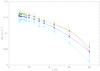Fig. 4 Derived nonthermal linewidth dV0 at Rv = 300 AU as a function of assumed kinetic temperature profile. T0 is the temperature at Rt = 300 AU. The 4 curves correspond to different exponents q = 0 (red), 0.2 (green), 0.4 (blue), and 0.6 (cyan). Errorbars are  ± 1σ.

To strengthen this conclusion, as our main goal is to constrain δV_tu(r), we also explored a much wider range of possible temperature profiles, varying T₀ and q. Results for dV₀ as a function of assumed T₀ are given in Fig. 4 for four values of q = 0,0.2,0.4, and 0.6. In each case, because the exponent e_v is not well constrained, we assumed e_v = q/2, which corresponds to a constant Mach number. Figure 4 shows that, unless the kinetic temperature is very high, the nonthermal linewidth must be  ≃ 0.10–0.15 km s^-1 to represent the observations.

Fig. 5 Predicted CS J = 5–4 line flux from the best fit models derived from CS J = 3–2 observations, as a function of assumed kinetic temperature profile. The 4 curves corresponding to the different exponents q = 0, 0.2, 0.4, and 0.6 are essentially degenerate. Errorbars are  ± 1σ. The shaded gray area indicates the measured line flux and its  ± 1σ range. Calibration uncertainty is not included.

The CS(3–2) data set itself suggests low temperatures, but the surface density profile is essentially flat (p = 0.14 ± 0.20), so the constraint may be considered as relatively weak. The temperature found with CS(3–2) is quite compatible with the one determined from CCH (Henning et al. 2010) and CN and HCN (Chapillon et al. 2012b). Moreover, the CS(5-4) data, although quite noisy, can be used to rule out high temperatures. Figure 5 shows the integrated line flux for the CS(5–4) data using the best fit parameters found from CS(3–2) as function of T₀ and q. Clearly, high temperatures (>20 K) can be ruled out, since they would produce a much brighter CS(5–4) emission than observed. This is consistent with the temperature derived from other tracers, although subthermal excitation of the CS(5–4) in a warmer medium cannot be ruled out¹.

Low temperatures are thus strongly suggested, although not firmly proven, by this study. In any case, the uncertainties on temperature profile have a negligible influence on the key parameters of this study, dV₀, as well as on p_CS. However, they can affect the derived CS column density by a factor 1.5–2.

3.3. A more realistic approach?

The assumption of homogeneous vertical mixing (constant abundance as a function of z) is a strong prior. In practice, chemical models predict that molecules are strongly depleted in the disk plane, owing to the condensation of volatiles on dust grains. Thus, the emission of molecules is expected to come from one or two scale heights above the disk plane. As the scale height is typically 10% of the radius, this means the emission comes from regions inclined  ± δi ≃ 6° from the disk midplane. Because the line of sight velocity is proportional to sin(i), these two different inclinations result in a broadening of the projected linewidth, which is not properly reproduced by the assumption of no vertical abundance gradient. This is essentially as if the emission came from two disks, one inclined by i + δi and the other by i − δi along the line of sight (see Semenov et al. 2008). To first order, the extra broadening due to these inclination differences would then be proportional to the rotation velocity, i.e. would decrease as $\sqrt{\mathrm{(}}\mathit{r}\mathrm{)}$, if δi is constant. The exponent of the nonthermal linewidth law e_v (see Eq. (9)) derived above is indeed quite close to the Keplerian exponent 0.5 (but with little significance).

In practice, δi will vary with radius. On one hand, h(r)/r increases slowly with r (as  ≈ r^0.25). On the other, the height above which molecules are found is expected to decrease in the outer parts of the disk, because (interstellar or scattered) UV photons can penetrate deeper towards the disk plane. This leads to enhanced photodesorption, and brings the molecular layer closer to the disk plane. As a consequence, the resulting increase in inclination spread is smaller in the outer regions than closer to the star. This could also contribute to the apparent decrease in the nonthermal broadening found previously by our simple analysis.

It is thus essential to check whether nonthermal motions are also required to explain the observations when CS is confined above the disk midplane. Although sophisticated chemical models exist, they require a prior knowledge of the H₂ density structure. This density structure is still very uncertain, and parametric chemical models (which would explore a range of possible solutions) do not yet exist in this respect.

We thus adopted a second parametrization of the CS emission from the disk, Model B, which differs from Model A in two ways. The CS surface density is no longer a power law. Instead, the disk surface density (dominated by molecular hydrogen) follows an exponentially tapered law ${\mathrm{\Sigma }}_{\mathrm{H}}\mathrm{\left(}\mathit{r}\mathrm{\right)}\mathrm{=}{\mathrm{\Sigma }}_{\mathrm{0}}{\left(\frac{\mathit{r}}{{\mathit{R}}_{\mathrm{0}}}\right)}^{\mathrm{-}\mathit{\gamma }}\exp \mathrm{(}\mathrm{-}\mathrm{(}\mathit{r}\mathit{/}{\mathit{R}}_{\mathrm{c}}{\mathrm{)}}^{\mathrm{2}\mathrm{-}\mathit{\gamma }}\mathrm{)}\mathit{,}$(12)which is the self-similar solution of the disk evolution when the viscosity is a (time constant) power law of radius (Lynden-Bell & Pringle 1974). CS is then assumed to only be present when the hydrogen column density from the current point towards the disk exterior (perpendicular to the disk midplane) is lower than some given threshold, Σ_d, the depletion threshold. In regions where CS exists, we further assume that its abundance is only a power law of radius. The disk is assumed to be vertically isothermal. The column density above a given height z is then given by ${\mathrm{\Sigma }}_{\mathrm{\infty }}\mathrm{\left(}\mathit{r,z}\mathrm{\right)}\mathrm{=}{\mathrm{\int }}_{\mathit{z}}^{\mathrm{\infty }}\mathit{n}\mathrm{\left(}\mathit{r,u}\mathrm{\right)}\mathrm{d}\mathit{u}\mathrm{=}\frac{\mathrm{\Sigma }\mathrm{\left(}\mathit{r}\mathrm{\right)}}{\mathrm{2}}\left(\mathrm{1}\mathrm{-}\mathrm{erf}\left(\frac{\mathit{z}}{\mathit{H}\mathrm{\left(}\mathit{r}\mathrm{\right)}}\right)\right)\mathit{,}$(13)from which the depletion height z_d(r) can be recovered as a function of Σ_d/Σ(r) ${\mathit{z}}_{\mathrm{d}}\mathrm{\left(}\mathit{r}\mathrm{\right)}\mathrm{=}\mathit{H}\mathrm{\left(}\mathit{r}\mathrm{\right)}\hspace{0.17em}{\mathrm{erf}}^{-1}\left(\mathrm{1}\mathrm{-}\frac{\mathrm{2}{\mathrm{\Sigma }}_{\mathrm{d}}}{\mathrm{\Sigma }\mathrm{\left(}\mathit{r}\mathrm{\right)}}\right)\mathrm{·}$(14)The CS abundance is therefore given by 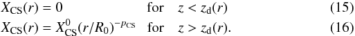$\begin{array}{ccc}& & {\mathit{X}}_{\mathrm{CS}}\mathrm{\left(}\mathit{r}\mathrm{\right)}\mathrm{=}\mathrm{0}\hspace{0.17em}\mathrm{for} \mathit{z}\mathit{<}{\mathit{z}}_{\mathrm{d}}\mathrm{\left(}\mathit{r}\mathrm{\right)}\\ & & {\mathit{X}}_{\mathrm{CS}}\mathrm{\left(}\mathit{r}\mathrm{\right)}\mathrm{=}{\mathit{X}}_{\mathrm{CS}}^{\mathrm{0}}\mathrm{(}\mathit{r}\mathit{/}{\mathit{R}}_{\mathrm{0}}{\mathrm{)}}^{\mathrm{-}{\mathit{p}}_{\mathrm{CS}}}\hspace{0.17em}\mathrm{for} \mathit{z}\mathit{>}{\mathit{z}}_{\mathrm{d}}\mathrm{(}\mathit{r}\mathrm{)}\mathit{.}\end{array}$\arraycolsep1.75ptIn this model, the overall surface density of CS thus follows the law 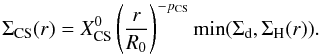${\mathrm{\Sigma }}_{\mathrm{CS}}\mathrm{\left(}\mathit{r}\mathrm{\right)}\mathrm{=}{\mathit{X}}_{\mathrm{CS}}^{\mathrm{0}}{\left(\frac{\mathit{r}}{{\mathit{R}}_{\mathrm{0}}}\right)}^{\mathrm{-}{\mathit{p}}_{\mathrm{CS}}}\begin{array}{}\min \end{array}\mathrm{\left(}{\mathrm{\Sigma }}_{\mathrm{d}}\mathit{,}{\mathrm{\Sigma }}_{\mathrm{H}}\mathrm{\right(}\mathit{r}\mathrm{\left)}\mathrm{\right)}\mathit{.}$(17)In the modeling, R_c and γ are fixed parameters. We used R_c = 180 AU and γ = 0.55, which were found by Guilloteau et al. (2011) from high-resolution, dual-frequency continuum, and Σ₀ is also taken from this article to obtain a disk mass of 0.03   M_⊙, which gives Σ₀(100   AU) = 9.6 × 10²³ cm^-2 (H₂ molecules).

Although imposing the density structure could allow non-LTE modeling to be performed, considering the large uncertainties on the real density structure², CS is assumed to be thermalized because densities are in general high enough, even at one to two scale heights. The remaining free parameters are now ${\mathit{X}}_{\mathrm{CS}}^{\mathrm{0}}$, p_CS, T₀, q, R_out, the turbulent width dV₀ (e_V being poorly constrained, we used e_V = q/2, a constant Mach number), and the depletion threshold Σ_d.

Although the rationale for the choice of parameters is based on behaviors predicted by chemical models, it is important to stress that our approach is still purely parametric. In particular, we make no a priori link between the thermal structure of the disk and the location of molecules.

The optimal value of Σ_d was first located through a grid of best-fit solutions computed with δV and Σ_d and T₀ as fixed parameters, and ${\mathit{X}}_{\mathrm{CS}}^{\mathrm{0}}$, p_CS and R_out as free parameters. The temperature was set to the best-fit solution found for the power law; similar results were obtained when allowing the temperature law to vary. This grid search did not reveal any secondary minimum. We then started from the best fit found in this grid search to proceed with a global fit of the parameters, including the temperature law. The best fit results are presented in Table 1. This model provides a slightly better fit to the CS(3–2) data than the power-law case.

3.3.1. Turbulent width

We find a nonthermal component slightly smaller than that derived in the power-law case, but still significant dV₀ = 0.11 ± 0.015 km s^-1 for H₀ = 16 AU. A lower value is expected, since part of the spatial extent at a given velocity is due to the spread in inclinations, which is larger in Model B than in Model A (which assumed vertically uniform CS abundances).

3.3.2. Depletion column density

The best fit “depletion” column density is Σ_d = 10^{21.7 ± 0.1} cm^-2. However, interpretation of this value is not straightforward. Changing the scale height from 16 AU (at 100 AU) to 8 or 32 AU does not significantly affect the derived Σ_d. This indicates that Σ_d is not constrained by the geometry alone. In fact, this value is found because the CS(3–2) images are apparently better represented by a simple power law for the CS surface density than by the more complex radial profiles that can result from the hypotheses made in Model B. With Σ_d ≃ 10²² cm^-2 and a power law for the CS abundance, the CS surface density behaves as a power law (of exponent p = 0.4 ± 0.2) out to R ≈ 400 AU, close enough to the outer radius of the CS distribution. With H₀ = 16 AU, model B also leads to slightly higher (but less constrained) temperatures than Model A, around 10 ± 2 K at 300 AU.

3.3.3. Vertical location

Although Σ_d is mostly constrained by the radial brightness profile in this case, it does not imply that the vertical distribution is not constrained. Starting from the best fit of the radial CS distribution, we can actually get an estimate of the system geometry by treating the scale height as a free parameter. We find H₀ = 9 ± 1.5 (see Table 1), which is consistent with the temperature derived from CS, which indicates H₀ = 10.4 ± 1.2. The required turbulent width increases when the scale height is diminished. The depletion height z_d derived from this best fit is plotted in Fig. 6, together with the corresponding value of Σ_d. It is important to note that the shape of z_d is prescribed by our model assumptions. In reality, the distribution of molecules can be substantially different, but our analysis nevertheless indicates that a substantial fraction of the CS molecules must reside around one scale height.

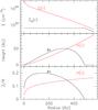Fig. 6 Top: total disk surface density Σ(r) and column density Σd(r) above the depletion height zd(r). Middle: depletion height zd(r) as a function of radius in the best fit model. The scale height H(r) is also indicated (in red). Bottom: as above, but for zd(r)/r and H(r)/r.

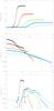Fig. 7 Predicted distribution of Temperature (top), H2 (middle) and CS (bottom) molecule densities as a function of height for several radii: 50 (black), 100 (red), 200 (green), 300 (blue), and 500 AU (cyan).

3.4. Comparison with chemical models

A chemical model for sulfur bearing molecules was developed by Dutrey et al. (2011) to explain the integrated line profiles obtained with the IRAM 30-m. The model predictions were done with the NAUTILUS code (Hersant et al. 2009), which computes the chemical composition of the gas and interstellar ices as a function of time. Bimolecular reactions between gas-phase species and interactions with direct UV photons and cosmic-ray particles, as well as UV photons induced by cosmic-rays, are considered, with a network of 4406 reactions for 460 species. Interactions with grain surfaces (including direct and UV induced dissociations), as well as reactions at the surfaces, through 1773 reactions, determine the abundance of 195 surface species. The NAUTILUS code is run in the vertical 1D approximation at different radii of the disk (from 50 to 500 AU). More details on the model parameters and the physical structure of the disk can be found in Dutrey et al. (2011). The observations of CS presented in this paper have been compared to the Case C for DM Tau of Dutrey et al. (2011, see their Tables 4 and 5).

Although this model does not use the same underlying density structure, it is interesting to compare its predictions to the results derived from the Plateau de Bure data. Figure 7 shows the distribution of CS molecules and the H₂ density and temperature vertical profiles for several radii. The range of heights at which CS is found corresponds to an H₂ column density towards the outside, Σ_∞(r,z) in the range of 10²² − 10²³ cm^-2, except at 50 AU where the warmer interior leads to enhanced CS abundance at larger depths.

The temperature is not the key parameter defining the molecular-rich layer. CS exists at temperatures well below its evaporation temperature (30 K), as can be seen in Fig. 7. The penetration of UV radiation (scattered from the star and coming from the ISM) is more important in defining this layer, which is limited by photodesorption near the disk plane and photodestruction of all molecules near the disk surface. Temperature effects become significant only above 30 K, for which high CS densities can be reached because of thermal desorption.

The enhanced CS surface density within 50 AU from the star is not probed by our observations, which are mostly sensitive to the 100–500 AU region. In this region, the predicted column density increases slightly with radius (see Dutrey et al. 2011, Fig. 4), while the analysis of our observations indicates a roughly constant or slightly decreasing column density. The chemical model does not include any radial or vertical mixing, that would be a natural consequence of the observed turbulent velocities. Vertical mixing will on average decrease the altitude at which CS molecules are found, while radial mixing will smooth out the CS abundance distribution. Consequently, radial mixing would tend to make the slope of the CS surface density profile closer to the one of H₂ that is expected to vary roughly as 1/r. This smoothing effect due to mixing can be seen in the study of Semenov & Wiebe (2011, see their Fig. 11), who investigated the impact of radial and vertical turbulent mixing. Semenov & Wiebe (2011) also find that the CS content can be increased by an order of magnitude by mixing. Higher angular resolutions (0.1–0.3′′) with ALMA are required to directly probe the inner disk region and prove (or disprove) our theoretical prediction of high CS abundance here.

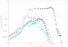Fig. 8 CS molecule density as a function of (essentially H2) column density for several radii: 50 (black), 100 (red), 200 (green), 300 (blue), and 500 AU (cyan).

The chemical models predict that CS molecules are located between z/r = 0.2 and 0.4 (see Fig. 7), while our best fit solution indicates z_d/r ≈ 0.15 − 0.2. When expressed as a function of Σ_d, the model predicts the range where CS is abundant reasonably well, a few 10²² to  ≈ 10²³ cm^-2 as shown by Fig. 8. The small discrepancies suggest that better agreement between the chemical model and the observations can be obtained by assuming larger dust grains and a geometrically thinner (i.e. colder) disk in the model. In this case, the molecular layer is expected to become closer to the disk plane (e.g. Aikawa & Nomura 2006), because of enhanced UV penetration and lower sticking efficiency. Dust settling would also bring the molecular layer in the same direction, by minimizing the sticking efficiency above the disk plane, but should be less important than grain growth since it only concerns the largest grains that offer less surface area per unit mass.

4. Discussion

The analysis presented above unambiguously indicates that a substantial additional line broadening is required besides the thermal component and that the derived magnitude of the turbulent motions is not too critically dependent on the assumptions about the location of the CS molecules.

In the simple power-law approach (Model A), using our temperature measurement, a mean molecular weight μ = 2.30, the derived sound speed is ${\mathit{C}}_{\mathrm{s}}\mathrm{\left(}\mathit{r}\mathrm{\right)}\mathrm{=}\sqrt{\mathit{kT}\mathrm{\left(}\mathit{r}\mathrm{\right)}\mathit{/}\mathit{\mu }{\mathit{m}}_{\mathrm{H}}}\mathrm{=}\mathrm{0.16}\mathrm{(}\mathit{r}\mathit{/}\mathrm{300} \mathrm{AU}{\mathrm{)}}^{-0.3}\hspace{0.17em}{\mathrm{km}\hspace{0.17em}\mathrm{s}}^{-1}$ (using the temperature derived from CS for the kinetic temperature), which corresponds to a Mach number M = δV_t/C_s/$\sqrt{\mathrm{2}}$ around 0.5 and a slightly lower value for Model B.

This result contrasts with the expectations from the α prescription of the viscosity, where the turbulent width is related to α in a way that depends on the nature of the turbulence. The value of δV ranges between a few αC_s to  ≈ $\sqrt{\mathit{\alpha }}{\mathit{C}}_{\mathrm{s}}$ (Cuzzi et al. 2001). All indirect measurements of the α parameter (Hartmann et al. 1998; Hueso & Guillot 2005; Guilloteau et al. 2011) indicate α values between a few 10^-4 and about 0.01, thus predicting much smaller turbulent widths, of at most 0.04 km s^-1 if extrapolated near 300 AU. However, these measurements often sample smaller regions. Hartmann et al. (1998) derive these from accretion rates, and are thus sensitive to the inner AUs only. The results of Hueso & Guillot (2005) and Guilloteau et al. (2011) are based on viscous spreading of the dust disk, and are mostly sensitive to the 100 AUs range.

Hughes et al. (2011) obtained a low value for TW Hya ( < 0.04 km s^-1), but up to 0.3 km s^-1 for the Herbig Ae star HD 163296 from CO J = 3–2 observations. An attractive explanation of these very different turbulence levels could have been the age difference between these two stars, with turbulence level decreasing with age as independently suggested by the Guilloteau et al. (2011) results. Our DM Tau result does not fit well in this scheme, as DM Tau is rather old, too. Differences in inclinations between the nearly face-on disk of TW Hya and the more inclined ones of DM Tau and HD 163296 could also play a role if the turbulence had significant anisotropy. However, shearing box simulations of MRI induced turbulence by Simon et al. (2011) show no evidence for such anisotropy. On the other hand, Flock et al. (2011) and Fromang & Nelson (2006) find small anisotropy, the radial velocity fluctuations being about 1.5–2 times larger than in the azimuthal or vertical directions.

It is tempting to ascribe the difference between the constraints on α (sampling the disk plane) and our measured turbulence level (sampling 1–2 scale heights) to the stratification of turbulence predicted by MHD models. Fromang & Nelson (2006) and Flock et al. (2011) show that the velocity dispersion increases quickly with height above two scale heights (with the c_s/Ω_K definition, i.e. at $\sqrt{\mathrm{2}}\mathit{H}\mathrm{\left(}\mathit{r}\mathrm{\right)}$ with our definition). However, they only reach a Mach number of 0.4 at four scale heights (3H(r)), which appears insufficient to explain our result.

The discrepancy between the apparent linewidths and the estimates of the viscosity may also point towards a weakness in our theoretical understanding of the turbulence. The turbulent width measures velocity dispersion, while the α viscosity measures a transport coefficient. They are related through the effective mixing length (Prandtl 1925), which may not be a simple function of α and H, as is usually assumed in the α model. In other words, the aforementioned relation between the turbulent Mach number and α may reach its limits in the disk outer parts. It is worth pointing out that the TW Hya disk is small (outer radius 230 AU), while those of HD 163296 and DM Tau are large (>600 AU and 900 AU, respectively). The smaller turbulent width found in TW Hya is consistent with the idea that viscous spreading is the main driver for the disk size. Measurements of the nonthermal linewidths for a wider sample of objects with different disk radii would be important in establishing this potential link.

It is also important to realize that, in all the analysis of the molecular line emission, the so-called “turbulent” width is an adjustable parameter that is used to fit deviations from the simple Keplerian disk model with purely thermal line broadening. Departure from these ideal conditions will affect the derived “turbulent” width. For example, we have explored in Sect. 3 the impact of the location of molecules above the disk plane, but other effects can exist. Small deviations from Keplerian rotation, which are ignored in our analysis, would have no impact on the linewidth for a nearly face-on object like TW Hya, but could affect more inclined objects like DM Tau (i = 35°) or HD163296 (i = 45°). Our study of the depletion depth in Sect.3 suggests that disk warps would, however, need to be quite significant (~10°) before affecting the required turbulent component.

5. Summary

Using the IRAM Plateau de Bure interferometer, we imaged the CS (3–2) emission from the disk of DM Tau at  ~1′′ resolution. Although noisy, CS(5–4) data obtained with the 30-m and at 2.5′′ resolution from the PdBI preclude temperatures exceeding about 20–30 K. The morphology of the emission indicates a significant local linewidth, around 0.14 km s^-1 near 300 AU. This result appears robust with respect to the assumed location of CS molecules above the disk’s midplane. While the magnitude of this linewidth is in agreement with measurements previously obtained by Piétu et al. (2007) and Chapillon et al. (2012b) from other molecules like HCO⁺, CN, HCN or CO isotopologues, the relatively large molecular weight of CS (44), combined with the temperature estimate and an accurate handling of the spectral response of the correlator, leaves no doubt here that this local linewidth is essentially due to a nonthermal (turbulent) component. The magnitude of these turbulent motions corresponds to a Mach number around 0.3–0.5.

Our data confirm the relatively low temperatures derived from other molecules such as CN, HCN, and CCH. (Chapillon et al. 2012b; Henning et al. 2010). They also suggest the CS molecules are located above one scale height from the disk plane, in reasonable agreement with predictions from chemical models.

This work shows the potential of CS as a turbulence tracer. No other molecules detected so far (including the recently reported HC₃N, Chapillon et al. 2012a) is both heavy and abundant enough to provide a more sensitive tracer. Also, CS offers a number of transitions in the mm/submm domain, which probe critical densities ranging from a few 10⁵ to several 10⁸ cm^-3. This, combined with its expected location in the molecular-rich layer, make this molecule a key probe of physical conditions in disks. The constraint obtained for the geometric location of CS molecules with respect to the disk plane, although still difficult to interpret, clearly indicates the potential of ALMA for probing different depths.

Acknowledgments

We thank the Plateau de Bure staff for performing the observations. This work was supported by the National Program PCMI from INSU-CNRS. D.S. acknowledges support by the Deutsche Forschungsgemeinschaft through SPP 1385: “The first ten million years of the solar system – a planetary materials approach” (SE 1962/1-2).

References

All Tables

All Figures

	Fig. 1 Channel maps of the CS J = 3–2 emission towards DM Tau. The angular resolution is 1.4′′ × 1.0′′ and the spectral resolution 0.16 km s-1. Contour spacing is 10 mJy/beam, corresponding to 2σ and 0.4 K brightness. The cross indicates the position, orientation, and aspect ratio of the dust disk.
In the text

	Fig. 2 Spectrum of CS J = 5–4 line towards DM Tau. The angular resolution is 3.5′′ and the spectral resolution 0.25 km s-1. The curve is a best-fit Gaussian to emphasize the detection.
In the text

	Fig. 3 Regions of the disk that yield equal projected velocities vobs. The ellipse is the projection of the disk’s outer edge.
In the text

	Fig. 4 Derived nonthermal linewidth dV0 at Rv = 300 AU as a function of assumed kinetic temperature profile. T0 is the temperature at Rt = 300 AU. The 4 curves correspond to different exponents q = 0 (red), 0.2 (green), 0.4 (blue), and 0.6 (cyan). Errorbars are  ± 1σ.
In the text

	Fig. 5 Predicted CS J = 5–4 line flux from the best fit models derived from CS J = 3–2 observations, as a function of assumed kinetic temperature profile. The 4 curves corresponding to the different exponents q = 0, 0.2, 0.4, and 0.6 are essentially degenerate. Errorbars are  ± 1σ. The shaded gray area indicates the measured line flux and its  ± 1σ range. Calibration uncertainty is not included.
In the text

	Fig. 6 Top: total disk surface density Σ(r) and column density Σd(r) above the depletion height zd(r). Middle: depletion height zd(r) as a function of radius in the best fit model. The scale height H(r) is also indicated (in red). Bottom: as above, but for zd(r)/r and H(r)/r.
In the text

	Fig. 7 Predicted distribution of Temperature (top), H2 (middle) and CS (bottom) molecule densities as a function of height for several radii: 50 (black), 100 (red), 200 (green), 300 (blue), and 500 AU (cyan).
In the text

	Fig. 8 CS molecule density as a function of (essentially H2) column density for several radii: 50 (black), 100 (red), 200 (green), 300 (blue), and 500 AU (cyan).
In the text

References

- Aikawa, Y. 2007, ApJ, 656, L93 [NASA ADS] [CrossRef] [Google Scholar]
- Aikawa, Y., & Nomura, H. 2006, ApJ, 642, 1152 [NASA ADS] [CrossRef] [Google Scholar]
- Andrews, S. M., Wilner, D. J., Hughes, A. M., et al. 2012, ApJ, 744, 162 [NASA ADS] [CrossRef] [Google Scholar]
- Balbus, S. A., & Hawley, J. F. 1991, ApJ, 376, 214 [NASA ADS] [CrossRef] [Google Scholar]
- Beckwith, S. V. W., Henning, T., & Nakagawa, Y. 2000, Protostars and Planets IV, 533 [Google Scholar]
- Carr, J. S., Tokunaga, A. T., & Najita, J. 2004, ApJ, 603, 213 [NASA ADS] [CrossRef] [Google Scholar]
- Chapillon, E., Dutrey, A., Guilloteau, S., et al. 2012a, ApJ, 756, 58 [NASA ADS] [CrossRef] [Google Scholar]
- Chapillon, E., Guilloteau, S., Dutrey, A., Piétu, V., & Guélin, M. 2012b, A&A, 537, A60 [NASA ADS] [CrossRef] [EDP Sciences] [Google Scholar]
- Cuzzi, J. N., Hogan, R. C., Paque, J. M., & Dobrovolskis, A. R. 2001, ApJ, 546, 496 [NASA ADS] [CrossRef] [Google Scholar]
- Dartois, E., Dutrey, A., & Guilloteau, S. 2003, A&A, 399, 773 [NASA ADS] [CrossRef] [EDP Sciences] [Google Scholar]
- Dutrey, A., Guilloteau, S., & Guelin, M. 1997, A&A, 317, L55 [NASA ADS] [Google Scholar]
- Dutrey, A., Guilloteau, S., & Ho, P. 2007, Protostars and Planets V, 495 [Google Scholar]
- Dutrey, A., Wakelam, V., Boehler, Y., et al. 2011, A&A, 535, A104 [NASA ADS] [CrossRef] [EDP Sciences] [Google Scholar]
- Flock, M., Dzyurkevich, N., Klahr, H., Turner, N. J., & Henning, T. 2011, ApJ, 735, 122 [NASA ADS] [CrossRef] [Google Scholar]
- Fromang, S., & Nelson, R. P. 2006, A&A, 457, 343 [NASA ADS] [CrossRef] [EDP Sciences] [MathSciNet] [Google Scholar]
- Gammie, C. F. 1996, ApJ, 457, 355 [NASA ADS] [CrossRef] [Google Scholar]
- Guilloteau, S., Dutrey, A., Piétu, V., & Boehler, Y. 2011, A&A, 529, A105 [NASA ADS] [CrossRef] [EDP Sciences] [Google Scholar]
- Hartmann, L., Calvet, N., Gullbring, E., & D’Alessio, P. 1998, ApJ, 495, 385 [NASA ADS] [CrossRef] [Google Scholar]
- Henning, T. 2008, Phys. Scr. Vol. T, 130, 014019 [Google Scholar]
- Henning, T., Semenov, D., Guilloteau, S., et al. 2010, ApJ, 714, 1511 [NASA ADS] [CrossRef] [Google Scholar]
- Hersant, F., Wakelam, V., Dutrey, A., Guilloteau, S., & Herbst, E. 2009, A&A, 493, L49 [NASA ADS] [CrossRef] [EDP Sciences] [Google Scholar]
- Horne, K., & Marsh, T. R. 1986, MNRAS, 218, 761 [NASA ADS] [CrossRef] [Google Scholar]
- Hueso, R., & Guillot, T. 2005, A&A, 442, 703 [NASA ADS] [CrossRef] [EDP Sciences] [Google Scholar]
- Hughes, A. M., Wilner, D. J., Andrews, S. M., Qi, C., & Hogerheijde, M. R. 2011, ApJ, 727, 85 [NASA ADS] [CrossRef] [Google Scholar]
- Ilgner, M., & Nelson, R. P. 2006, A&A, 445, 223 [CrossRef] [EDP Sciences] [Google Scholar]
- Ilgner, M., Henning, T., Markwick, A. J., & Millar, T. J. 2004, A&A, 415, 643 [NASA ADS] [CrossRef] [EDP Sciences] [Google Scholar]
- Johansen, A., Oishi, J. S., Mac Low, M.-M., et al. 2007, Nature, 448, 1022 [Google Scholar]
- Johansen, A., Klahr, H., & Henning, T. 2011, A&A, 529, A62 [NASA ADS] [CrossRef] [EDP Sciences] [Google Scholar]
- Keller, C., & Gail, H.-P. 2004, A&A, 415, 1177 [NASA ADS] [CrossRef] [EDP Sciences] [Google Scholar]
- Lynden-Bell, D., & Pringle, J. E. 1974, MNRAS, 168, 603 [NASA ADS] [CrossRef] [Google Scholar]
- Oishi, J. S., Mac Low, M.-M., & Menou, K. 2007, ApJ, 670, 805 [NASA ADS] [CrossRef] [MathSciNet] [Google Scholar]
- Papaloizou, J. C. B., & Terquem, C. 2006, Rep. Prog. Phys., 69, 119 [Google Scholar]
- Piétu, V., Dutrey, A., & Guilloteau, S. 2007, A&A, 467, 163 [NASA ADS] [CrossRef] [EDP Sciences] [Google Scholar]
- Prandtl, L. 1925, Zs. Angew. Math. Mech., 5, 136 [Google Scholar]
- Regev, O., & Gitelman, L. 2002, A&A, 396, 623 [NASA ADS] [CrossRef] [EDP Sciences] [Google Scholar]
- Semenov, D., & Wiebe, D. 2011, ApJS, 196, 25 [NASA ADS] [CrossRef] [Google Scholar]
- Semenov, D., Wiebe, D., & Henning, T. 2006, ApJ, 647, L57 [NASA ADS] [CrossRef] [Google Scholar]
- Semenov, D., Pavlyuchenkov, Y., Henning, T., Wolf, S., & Launhardt, R. 2008, ApJ, 673, L195 [NASA ADS] [CrossRef] [Google Scholar]
- Simon, J. B., Armitage, P. J., & Beckwith, K. 2011, ApJ, 743, 17 [NASA ADS] [CrossRef] [Google Scholar]
- Tscharnuter, W. M., & Gail, H.-P. 2007, A&A, 463, 369 [NASA ADS] [CrossRef] [EDP Sciences] [Google Scholar]
- Uribe, A. L., Klahr, H., Flock, M., & Henning, T. 2011, ApJ, 736, 85 [NASA ADS] [CrossRef] [Google Scholar]
- Urpin, V. A. 1984, Sov. Ast., 28, 50 [Google Scholar]
- Voelk, H. J., Jones, F. C., Morfill, G. E., & Roeser, S. 1980, A&A, 85, 316 [NASA ADS] [Google Scholar]