© ESO, 2012

1. Introduction

It is anticipated that magnetic twist plays a considerable role in the structure of coronal loops. The highly dynamic photosphere and chromosphere can introduce twist in the magnetic field of the solar corona. For example, footpoint rotation and shear motion may result in twisting of coronal loops (see e.g., Brown et al. 2003). A newly emerged magnetic field is also supposed to be twisted during the buoyant evolution through the convection zone, meaning that loops may emerge already twisted (see e.g., Moreno-Insertis & Emonet 1996; Hood et al. 2009). Twist also considerably contributes to the eruption of many prominences and coronal mass ejections (CMEs; see e.g., Hood & Priest 1979; Priest et al. 1989).

In the theoretical analysis of magnetohydrodynamic (MHD) waves, the effects of a curved loop axis are usually omitted. The stability of straight tubes with twisted magnetic field has been investigated by e.g., Shafranov (1957), Kruskal et al. (1958), and Suydam (1958). The role of line tying conditions in the context of coronal loops has been studied by e.g., Raadu (1972) while the effect of gas pressure on the kink instability has been analysed by e.g., Giachetti et al. (1977). The combination of both effects has been studied by Hood & Priest (1979, 1981), Hood et al. (1982), Einaudi & van Hoven (1983), and Velli et al. (1990). More recently, Zaqarashvili et al. (2010) and Díaz et al. (2011) have considered the stability of twisted magnetic flux tubes with mass flows along the field lines. The main aim of the previous works is determining the instability threshold and calculating the growth rate of kink unstable modes.

Stable propagating MHD waves have been studied previously, but almost always under particular conditions that somehow reduce the mathematical complexity. Often the MHD waves are incompressible and/or the azimuthal component of the magnetic field varies linearly with distance up to a certain position where it drops to zero or all the way up to infinity. The first choice leads to a surface current while the second choice causes magnetic energy to diverge. Early studies were performed by Goossens et al. (1992) and Bennett et al. (1999) in the incompressible regime. The analysis of sausage modes (m = 0) has been carried out by Erdélyi & Fedun (2006, 2007). Kink modes assuming compressible motions have been considered by Erdélyi & Carter (2006), Carter & Erdélyi (2008), Erdélyi & Fedun (2010). In these works standing transverse waves have not been considered and only propagating waves have been analysed.

In particular, Ruderman (2007, see also review by Ruderman & Erdélyi 2009) studied standing waves and concluded that twist does not affect kink modes, only fluting modes are modified (see also Goossens et al. 1992). This result is due to the particular choice of constant magnetic twist, i.e., twist is independent of the radial coordinate. The conclusions of the work of Ruderman (2007) have some authors to regard twist as unimportant for transverse kink oscillations.

In this paper we study the effect of an azimuthal magnetic field component on the frequencies of MHD waves for an equilibrium model with nonconstant magnetic twist. We are especially interested in the effect of twist on standing kink modes, a problem that, to our knowledge, has not been addressed in the context of transverse coronal oscillations (with the exception of standing fluting modes, studied in Ruderman 2007). Thus, our focus is on the fingerprints of twist on transverse kink oscillations but in the stable regime. This might be relevant for interpreting kink oscillations, from the early transverse kink oscillations reported with TRACE (Aschwanden et al. 1999; Nakariakov et al. 1999), to the last AIA observations of transverse oscillating loops (Aschwanden & Schrijver 2011).

2. Equilibrium model of the magnetically twisted loop

The model for the coronal loop that we use in the present paper is a straight cylinder with constant density inside the cylinder and constant density outside the cylinder. Thus, the coronal loop is modelled as a density enhancement characterised by a density contrast ρ_i/ρ_e with ρ_i being the internal density and ρ_e the external density, $\begin{array}{ccc}\mathit{\rho }\mathrm{=}\{\begin{array}{c}\\ & \\ & \end{array}& & \end{array}$(1)At r = R the density changes in a discontinuous manner and R is the radius of the loop.

Under coronal conditions it is a good approximation to neglect plasma pressure compared to magnetic pressure. This zero-β approximation removes the slow magnetoacoustic waves from the analysis. In the present paper we allow the magnetic twist to be nonconstant. The model starts from the equation of magnetostatic equilibrium $\begin{array}{ccc}\frac{\mathrm{d}{\mathit{B}}^{\mathrm{2}}}{\mathrm{d}\mathit{r}}\mathrm{=}\mathrm{-}\mathrm{2}\frac{{\mathit{B}}_{\mathit{\varphi }}^{\mathrm{2}}}{\mathit{r}}\mathit{,}& & \end{array}$(2)where $\begin{array}{ccc}{\mathit{B}}^{\mathrm{2}}\mathrm{=}{\mathit{B}}_{\mathit{z}}^{\mathrm{2}}\mathrm{+}{\mathit{B}}_{\mathit{\varphi }}^{\mathrm{2}}\mathit{.}& & \end{array}$(3)Here the azimuthal component of the magnetic field is prescribed and Eq. (2) is solved for B_z(x) with x = r/R. The solution is $\begin{array}{ccc}{\mathit{B}}_{\mathit{z}}^{\mathrm{2}}\mathrm{\left(}\mathit{x}\mathrm{\right)}\mathrm{=}{\mathit{B}}_{\mathit{z}}^{\mathrm{2}}\mathrm{\left(}\mathrm{0}\mathrm{\right)}\mathrm{-}{\mathit{B}}_{\mathit{\varphi }}^{\mathrm{2}}\mathrm{\left(}\mathit{x}\mathrm{\right)}\mathrm{-}\mathrm{2}{\mathrm{\int }}_{\mathrm{0}}^{\mathit{x}}\frac{{\mathit{B}}_{\mathit{\varphi }}^{\mathrm{2}}\mathrm{\left(}\mathit{s}\mathrm{\right)}}{\mathit{s}}\mathrm{d}\mathit{s}\mathit{.}& & \end{array}$(4)The azimuthal component of the field is written as $\begin{array}{ccc}{\mathit{B}}_{\mathit{\varphi }}\mathrm{\left(}\mathit{x}\mathrm{\right)}\mathrm{=}\mathit{Af}\mathrm{\left(}\mathit{x}\mathrm{\right)}\mathit{,}& & \end{array}$(5)where A has the dimension of a magnetic field and f(x) is a dimensionless function satisfying the condition f(0) = 0 or better f(x) → 0 for x → 0. If we insert Eq. (5) in (4) we find $\begin{array}{ccc}{\mathit{B}}_{\mathit{z}}^{\mathrm{2}}\mathrm{\left(}\mathit{x}\mathrm{\right)}& \mathrm{=}& {\mathit{B}}_{\mathit{z}}^{\mathrm{2}}\mathrm{\left(}\mathrm{0}\mathrm{\right)}\mathrm{-}{\mathit{A}}^{\mathrm{2}}\mathit{G}\mathrm{\left(}\mathit{x}\mathrm{\right)}\mathit{,}\\ \mathit{G}\mathrm{\left(}\mathit{x}\mathrm{\right)}& \mathrm{=}& \end{array}$Notice that G(0) = 0 and G(x) ≥ 0.

A particular choice for f(x) used in the present paper is 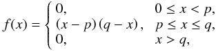$\begin{array}{ccc}\mathit{f}\mathrm{\left(}\mathit{x}\mathrm{\right)}\mathrm{=}\{\begin{array}{c}\\ & \\ & \\ & \end{array}& & \end{array}$(8)where p and q are constants that we can freely choose. The choice p = 0 is an option and that q > 1 is also allowed. For this model we have the freedom to have twist inside and also outside the tube. The function f(x) attains its maximal value f_max = (q − p)²/4 at x_m = (p + q)/2. Hence $\begin{array}{ccc}{\mathit{B}}_{\mathit{\varphi }}\mathrm{\left(}\mathit{x}\mathrm{\right)}\mathrm{=}\mathit{\alpha }{\mathit{B}}_{\mathit{z}}\mathrm{\left(}\mathrm{0}\mathrm{\right)}\frac{\mathit{f}\mathrm{\left(}\mathit{x}\mathrm{\right)}}{{\mathit{f}}_{\max }}\mathrm{·}& & \end{array}$(9)In order to relate the strength of the azimuthal component B_ϕ with respect to the dominant longitudinal component, we introduce α: $\begin{array}{ccc}\mathit{\alpha }\mathrm{=}\frac{{\mathit{B}}_{\mathit{\varphi ,}\max }}{{\mathit{B}}_{\mathit{z}}\mathrm{\left(}\mathrm{0}\mathrm{\right)}}\mathit{,}& & \end{array}$(10)hence $\begin{array}{ccc}\mathit{A}\mathrm{=}\frac{\mathit{\alpha }}{{\mathit{f}}_{\max }}{\mathit{B}}_{\mathit{z}}\mathrm{\left(}\mathrm{0}\mathrm{\right)}\mathit{.}& & \end{array}$(11)For the function f(x) specified by Eq. (8) it follows that 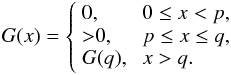$\begin{array}{ccc}\mathit{G}\mathrm{\left(}\mathit{x}\mathrm{\right)}\mathrm{=}\{\begin{array}{c}\\ & \\ & \\ & \end{array}& & \end{array}$(12)This function is calculated using Eq. (7).

In summary, the equilibrium magnetic field is defined as $\begin{array}{ccc}{\mathit{B}}_{\mathit{z}}\mathrm{=}{\mathit{B}}_{\mathrm{0}}\mathit{,}\hspace{0.17em}\hspace{0.17em}{\mathit{B}}_{\mathit{\varphi }}\mathrm{=}\mathrm{0}\mathit{,}& & \end{array}$(13)for x < p, $\begin{array}{ccc}{\mathit{B}}_{\mathit{z}}\mathrm{=}\sqrt{{\mathit{B}}_{\mathrm{0}}^{\mathrm{2}}\mathrm{-}{\mathit{A}}^{\mathrm{2}}\mathit{G}\mathrm{\left(}\mathit{x}\mathrm{\right)}}\mathit{,}\hspace{0.17em}\hspace{0.17em}{\mathit{B}}_{\mathit{\varphi }}\mathrm{=}\mathit{A}\mathrm{(}\mathit{x}\mathrm{-}\mathit{p}\mathrm{)}\mathrm{(}\mathit{x}\mathrm{-}\mathit{q}\mathrm{)}\mathit{,}& & \end{array}$(14)for p < x < q, with $\begin{array}{ccc}& & \mathit{G}\mathrm{\left(}\mathit{x}\mathrm{\right)}\mathrm{=}\mathrm{(}\mathit{x}\mathrm{-}\mathit{p}{\mathrm{)}}^{\mathrm{2}}\mathrm{(}\mathit{x}\mathrm{-}\mathit{q}{\mathrm{)}}^{\mathrm{2}}\mathrm{+}{\mathit{c}}_{\mathrm{4}}\mathrm{(}{\mathit{x}}^{\mathrm{4}}\mathrm{-}{\mathit{p}}^{\mathrm{4}}\mathrm{)}\mathrm{+}{\mathit{c}}_{\mathrm{3}}\mathrm{(}{\mathit{x}}^{\mathrm{3}}\mathrm{-}{\mathit{p}}^{\mathrm{3}}\mathrm{)}\\ & & \mathrm{+}{\mathit{c}}_{\mathrm{2}}\mathrm{(}{\mathit{x}}^{\mathrm{2}}\mathrm{-}{\mathit{p}}^{\mathrm{2}}\mathrm{)}\mathrm{+}{\mathit{c}}_{\mathrm{1}}\mathrm{(}\mathit{x}\mathrm{-}\mathit{p}\mathrm{)}\mathrm{+}{\mathit{c}}_{\mathit{l}}\left(\ln \mathrm{\left(}\mathit{x}\mathrm{\right)}\mathrm{-}\ln \mathrm{\left(}\mathit{p}\mathrm{\right)}\right)\mathit{,}\\ & & {\mathit{c}}_{\mathrm{1}}\mathrm{=}\mathrm{-}\mathrm{4}\mathit{pq}\mathrm{(}\mathit{p}\mathrm{+}\mathit{q}\mathrm{)}\mathit{,}\\ & & {\mathit{c}}_{\mathrm{2}}\mathrm{=}\mathrm{(}\mathit{p}\mathrm{+}\mathit{q}{\mathrm{)}}^{\mathrm{2}}\mathrm{+}\mathrm{2}\mathit{pq,}\\ & & {\mathit{c}}_{\mathrm{3}}\mathrm{=}\mathrm{-}\frac{\mathrm{4}}{\mathrm{3}}\mathrm{(}\mathit{p}\mathrm{+}\mathit{q}\mathrm{)}\mathit{,}\\ & & {\mathit{c}}_{\mathrm{4}}\mathrm{=}\frac{\mathrm{1}}{\mathrm{2}}\mathit{,}\\ & & {\mathit{c}}_{\mathit{l}}\mathrm{=}\mathrm{2}{\mathit{p}}^{\mathrm{2}}{\mathit{q}}^{\mathrm{2}}\mathit{,}\end{array}$ and $\begin{array}{ccc}{\mathit{B}}_{\mathit{\varphi }}\mathrm{=}\mathrm{0}\mathit{,}\hspace{0.17em}\hspace{0.17em}{\mathit{B}}_{\mathit{z}}\mathrm{=}\sqrt{{\mathit{B}}_{\mathrm{0}}^{\mathrm{2}}\mathrm{-}{\mathit{A}}^{\mathrm{2}}\mathit{G}\mathrm{\left(}\mathit{q}\mathrm{\right)}}\mathit{,}& & \end{array}$(21)for x > q.

3. MHD eigenmodes

3.1. MHD equations and numerical method

The motions superimposed on the equilibrium model given in the previous section are governed by the linearised ideal MHD equations in cylindrical coordinates. These equations can be found in the Appendix. Several terms involving radial derivatives of the equilibrium magnetic field are present in the equations.

In the MHD equations we have performed a Fourier analysis in time, with ω the frequency, and also in the azimuthal direction, m being the azimuthal wavenumber. For the longitudinal direction (along the tube axis) two situations are studied. The first situation corresponds to fully propagating waves, allowing Fourier decomposition in z, k being the longitudinal wavenumber. In this case the equations are solved in the radial coordinate r. The second situation corresponds to standing waves with line-tying conditions at the footpoints of the loop. This problem does not allow Fourier analysis in z, and the equations are solved in 2D (in r and z). For the analysis of propagating waves the system of equations reduces in the ideal regime to the Hain-Lüst equation. In general, it is not possible to find analytical solutions to this equation when the twist profile is nonconstant. For this reason the MHD equations are numerically solved using the code PDE2D (Sewell 2005) in the two situations (1D and 2D) explained above. More details about the numerical method can be found in Terradas et al. (2006). In the present paper we avoided possible Alfvénic resonances on purpose, interesting as they might be. In addition, we stayed away from a strong azimuthal field that can cause kink instabilities of the magnetic flux tube. This means that the eigenfrequency ω is a purely real magnitude in our analysis.

3.2. Effect of the azimuthal magnetic field on MHD waves

Since we adopted the zero-β approximation, the only characteristic frequency in the system is the local Alfvén frequency ω_A. The effect that the azimuthal component of the magnetic field B_ϕ has on the MHD waves can be appreciated from the effect of B_ϕ on ${\mathit{\omega }}_{\mathrm{A}}^{\mathrm{2}}$. The square of the Alfvén frequency is defined as $\begin{array}{ccc}{\mathit{\omega }}_{\mathrm{A}}^{\mathrm{2}}\mathrm{=}\frac{\mathrm{1}}{{\mathit{\mu }}_{\mathrm{0}}\mathit{\rho }}{\left(\frac{\mathit{m}}{\mathit{r}}{\mathit{B}}_{\mathit{\varphi }}\mathrm{+}\mathit{k}{\mathit{B}}_{\mathit{z}}\right)}^{\mathrm{2}}\mathit{.}& & \end{array}$(22)This expression can be written as $\begin{array}{ccc}{\mathit{\omega }}_{\mathrm{A}}^{\mathrm{2}}\mathrm{=}\frac{{\mathit{B}}_{\mathit{z}}^{\mathrm{2}}}{{\mathit{\mu }}_{\mathrm{0}}\mathit{\rho }}\frac{\mathrm{1}}{{\mathit{R}}^{\mathrm{2}}}\mathrm{(}\mathit{kR}{\mathrm{)}}^{\mathrm{2}}{\left(\mathrm{1}\mathrm{+}\frac{\mathit{m}}{\mathit{\pi }}\mathrm{\Phi }\mathrm{\left(}\mathit{r}\mathrm{\right)}\right)}^{\mathrm{2}}\mathit{.}& & \end{array}$(23)The function Φ(r) is $\begin{array}{ccc}\mathrm{\Phi }\mathrm{\left(}\mathit{r}\mathrm{\right)}\mathrm{=}\frac{\mathit{\pi }}{\mathit{kR}}\frac{{\mathit{B}}_{\mathit{\varphi }}}{\mathrm{(}\mathit{r}\mathit{/}\mathit{R}\mathrm{)}{\mathit{B}}_{\mathit{z}}}\mathrm{=}\mathit{L}\frac{{\mathit{B}}_{\mathit{\varphi }}}{\mathit{r}{\mathit{B}}_{\mathit{z}}}\mathit{,}& & \end{array}$(24)where we have defined L that k = π/L. Φ(r) is the twist of the magnetic field lines and it is 2π times the number of windings of the field around the loop axis over a distance L. Equation (23) suggests that even a relatively small ϕ-component of the magnetic field in the sense that  | B_ϕ |  ≪  | B_z | , might have a relatively important effect on the MHD waves. The relative importance of B_ϕ to B_z is controlled by the amount of twist of the magnetic field, with the length L being a relevant factor.

The ratio of the contribution to the Alfvén frequency due to the azimuthal component B_ϕ to that due to the longitudinal component is $\begin{array}{ccc}\frac{\mathit{m}}{\mathit{kR}}\frac{{\mathit{B}}_{\mathit{\varphi }}}{\mathrm{(}\mathit{r}\mathit{/}\mathit{R}\mathrm{)}{\mathit{B}}_{\mathit{z}}}\mathrm{·}& & \end{array}$(25)We computed the maximal value of the ratio for the model discussed in Sect. 2. We considered a weak azimuthal field and a relatively low value of α ≪ 1. To first order in α (small α approximation) $\begin{array}{ccc}{\mathit{B}}_{\mathit{z}}& \mathrm{\simeq }& {\mathit{B}}_{\mathit{z}}\mathrm{\left(}\mathrm{0}\mathrm{\right)}\mathit{,}\\ {\mathit{B}}_{\mathit{\varphi }}& \mathrm{=}& \mathit{\alpha }{\mathit{B}}_{\mathit{z}}\mathrm{\left(}\mathrm{0}\mathrm{\right)}\mathit{f}\mathrm{\left(}\mathit{x}\mathrm{\right)}\mathit{/}{\mathit{f}}_{\max }\mathit{.}\end{array}$Hence $\begin{array}{ccc}\frac{{\mathit{B}}_{\mathit{\varphi }}}{\mathrm{(}\mathit{r}\mathit{/}\mathit{R}\mathrm{)}{\mathit{B}}_{\mathit{z}}}\mathrm{=}\mathit{\alpha }\frac{\mathit{f}\mathrm{\left(}\mathit{x}\mathrm{\right)}}{\mathit{x}}\frac{\mathrm{1}}{{\mathit{f}}_{\max }}\mathrm{·}& & \end{array}$(28)For the prescription of f(x) given by Eq. (8) we already know the value of x_m and f_max. In addition, the function f(x)/x is maximal at ${\mathit{x}}_{\mathrm{\ast }}\mathrm{=}\sqrt{\mathit{pq}}$, and $\mathit{f}\mathrm{\left(}{\mathit{x}}_{\mathrm{\ast }}\mathrm{\right)}\mathit{/}{\mathit{x}}_{\mathrm{\ast }}\mathrm{=}\mathit{p}\mathrm{+}\mathit{q}\mathrm{-}\mathrm{2}\sqrt{\mathit{pq}}$. Hence the maximal value of $\begin{array}{ccc}{\frac{{\mathit{B}}_{\mathit{\varphi }}}{\mathrm{(}\mathit{r}\mathit{/}\mathit{R}\mathrm{)}{\mathit{B}}_{\mathit{z}}}|}_{\max }\mathrm{=}\mathit{\alpha }\frac{\mathrm{4}}{{\left(\mathit{q}\mathrm{-}\mathit{p}\right)}^{\mathrm{2}}}\left(\mathit{p}\mathrm{+}\mathit{q}\mathrm{-}\mathrm{2}\sqrt{\mathit{pq}}\right)\mathit{.}& & \end{array}$(29)For example, for the values p = 1/2 and q = 3/2 used in our calculations we find that $\begin{array}{ccc}{\frac{\mathit{m}}{\mathit{kR}}\frac{{\mathit{B}}_{\mathit{\varphi }}}{\mathrm{(}\mathit{r}\mathit{/}\mathit{R}\mathrm{)}{\mathit{B}}_{\mathit{z}}}|}_{\max }\mathrm{\approx }\mathrm{1.08}\hspace{0.17em}\mathit{m}\hspace{0.17em}\frac{\mathit{\alpha }}{\mathit{kR}}\mathrm{·}& & \end{array}$(30)As an example we consider a loop that is 10 times longer than the radius. For the fundamental mode along the tube axis it follows that kR = π/10. So for α = 1/10 the ratio is about 0.34. Thus, although the azimuthal component of the magnetic field is weak, its effect on the Alfvén frequency is substantial. For realistic loops it is a competition between the two quantities kR and α which determine the ultimate effect.

We omitted resonantly damped eigenmodes. This choice restricts the maximal twist allowed in the system or conversely the allowed combinations of α and kR. Even for a constant density profile like the one considered in this work (see Eq. (1)), ω_A is a function of position because B_ϕ varies with position and the corresponding term is multiplied by the factor 1/r. A necessary (but not sufficient) condition for the absence of resonances is that $\max {\mathit{\omega }}_{\mathrm{Ai}}^{\mathrm{2}}\mathrm{\le }\min {\mathit{\omega }}_{\mathrm{Ae}}^{\mathrm{2}}$. This conditions is equivalent to $\begin{array}{ccc}\begin{array}{}\max \end{array}\mathrm{\Phi }\mathit{<}\mathit{\pi }\left(\sqrt{{\mathit{\rho }}_{\mathrm{i}}\mathit{/}{\mathit{\rho }}_{\mathrm{e}}}\mathrm{-}\mathrm{1}\right)\mathit{.}& & \end{array}$(31) For ρ_i/ρ_e = 3 this implies that maxΦ ≲ 0.73π.

Condition (31) can be rewritten in terms of the function f(x) as $\begin{array}{ccc}\frac{\mathit{\alpha }}{\mathit{kR}}\mathit{<}{\mathit{x}}_{\mathrm{\ast }}\frac{{\mathit{f}}_{\max }}{\mathit{f}\mathrm{\left(}{\mathit{x}}_{\mathrm{\ast }}\mathrm{\right)}}\left(\sqrt{{\mathit{\rho }}_{\mathrm{i}}\mathit{/}{\mathit{\rho }}_{\mathrm{e}}}\mathrm{-}\mathrm{1}\right)\mathit{.}& & \end{array}$(32)For the typical values that we use in the computations the inequality is α/kR ≲ 0.67. So we can define the critical value of α as $\begin{array}{ccc}{\mathit{\alpha }}_{\mathit{J}}\mathrm{=}\mathit{kR}\hspace{0.17em}{\mathit{x}}_{\mathrm{\ast }}\frac{{\mathit{f}}_{\max }}{\mathit{f}\mathrm{\left(}{\mathit{x}}_{\mathrm{\ast }}\mathrm{\right)}}\left(\sqrt{{\mathit{\rho }}_{\mathrm{i}}\mathit{/}{\mathit{\rho }}_{\mathrm{e}}}\mathrm{-}\mathrm{1}\right)\mathit{.}& & \end{array}$(33)Then for values α > α_J the azimuthal component of the magnetic field introduces resonances even in configurations with constant density. In addition to α_J we can consider the situation when the azimuthal component B_ϕ dominates the variation of ${\mathit{\omega }}_{\mathrm{A}}^{\mathrm{2}}$. For m = 1 this happens when maxΦ(r) ≥ π (see Eq. (25)). For the function f(x) defined in Eq. (8) this can be reformulated into $\begin{array}{ccc}\frac{\mathit{\alpha }}{\mathit{kR}}\mathrm{\ge }{\mathit{x}}_{\mathrm{\ast }}\frac{{\mathit{f}}_{\max }}{\mathit{f}\mathrm{\left(}{\mathit{x}}_{\mathrm{\ast }}\mathrm{\right)}}\mathrm{·}& & \end{array}$(34)This forces us to define a second critical value for α$\begin{array}{ccc}{\mathit{\alpha }}_{\mathit{M}}\mathrm{=}\mathit{kR}\hspace{0.17em}{\mathit{x}}_{\mathrm{\ast }}\frac{{\mathit{f}}_{\max }}{\mathit{f}\mathrm{\left(}{\mathit{x}}_{\mathrm{\ast }}\mathrm{\right)}}\mathit{,}& & \end{array}$(35)which differers from α_J by the factor ($\sqrt{{\mathit{\rho }}_{\mathrm{i}}\mathit{/}{\mathit{\rho }}_{\mathrm{e}}}\mathrm{-}\mathrm{1}$). For the present model with p = 1/2 and q = 3/2, α_M ≃ 1.09   kR. Below we used sufficiently low values of α compared to α_J and α_M. This implies that even in the thin tube approximation we can use the small α approximation.

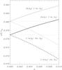Fig. 1 Frequency as a function of twist (α). The curves are obtained by solving the eigenvalue problem in 1D. The dotted line represents the solution for the untwisted case. For this particular example, ρi/ρe = 3, p = 1/2, q = 3/2. The two sets of solutions are associated to m = 1 and k1 = π/50R (thick lines), and k2 = π/48R (thin lines).

4. Results: propagating waves

We start by solving the eigenvalue problem for propagating waves using different pairs of the wavenumbers m and k, which are assumed to be positive. We use a particular choice of parameters, ρ_i/ρ_e = 3, p = 1/2, q = 3/2. In Fig. 1 the dependence of the eigenfrequency on α, which measures the amount of twist, is plotted. For the pair (m,k₁) the frequency is ω = k₁c_k when α = 0, i.e., we recover the known result in the absence of twist (in the thin tube approximation), which is the kink speed $\begin{array}{ccc}{\mathit{c}}_{\mathrm{k}}\mathrm{=}\sqrt{\frac{\mathrm{2}}{\mathrm{1}\mathrm{+}{\mathit{\rho }}_{\mathrm{e}}\mathit{/}{\mathit{\rho }}_{\mathrm{i}}}}{\mathit{v}}_{\mathrm{Ai}}\mathit{,}& & \end{array}$(36)where ${\mathit{v}}_{\mathrm{Ai}}\mathrm{=}{\mathit{B}}_{\mathrm{0}}\mathit{/}\sqrt{{\mathit{\mu }}_{\mathrm{0}}{\mathit{\rho }}_{\mathrm{i}}}$ is the internal Alfvén speed for a straight field.

Figure 1 shows that the frequency increases monotonically with α (see continuous thick line). Exactly the same curve is obtained for the wavenumbers ( − m, − k₁), meaning that the results are degenerate with respect to a change in sign of the two wavenumbers. In constrast, for ( − m,k₁) and (m, − k₁) the frequency decreases with α (see dashed thick line). This behaviour reflects the fact that, in contrast to the purely vertical magnetic field model, twist breaks the symmetry with respect to the propagation direction when the sign of one of the two wavenumbers is changed (see also the results of Vasheghani Farahani et al. 2010, for torsional Alfvén waves). The increase in frequency of the modes (m,k₁) and ( − m, − k₁) with respect to the un-twisted case is around 4% while the decrease for ( − m,k₁) and (m, − k₁) is 8% for α = 0.01. This means that a very weak twist (of about 1%) produces an effect on the frequency that is not negligible. The maximum value of α in our calculations has been chosen to satisfy that α < α_J and α < α_M for the reasons explained in Sect. 3.2.

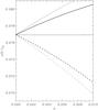Fig. 2 Frequency as a function of twist (α). For this particular example, ρi/ρe = 3, p = 1/2, q = 3/2 represented with thick lines while the case p = 0, q = 2 is plotted with thin lines. The dotted line represents the solution for the untwisted case. The horizontal continuous line is obtained by numerically solving the eigenvalue problem in 2D. The same notation as in Fig. 1 is used.

Figure 1 also suggests that a linear variation of ω with α is a good approximation of the actual dependency, $\begin{array}{ccc}\mathit{\omega }& \mathrm{\simeq }& \\ \mathit{\omega }& \mathrm{\simeq }& \end{array}$a being the slope of the linear approximation. The twist profiles considered by Goossens et al. (1992) and Ruderman (2007) are special since for those cases a = 0, i.e., there is no frequency change for different wavenumbers (for example, m =  ± 1). However, for nonconstant twist configurations, like those studied here, there is always a frequency split.

Similar behaviour occurs for different longitudinal wave numbers, the curves are just shifted vertically (see continuous and dashed thin lines). The slope of the curves is independent of the value of k, as we can see in Fig. 1 (compare the curves for k₁ and k₂), but as we show below, it depends on the particular twist profile. According to Fig. 1 for a fixed frequency and fixed value of twist, there are always four possible solutions, (m,k₁), ( − m, − k₁), ( − m,k₂), (m, − k₂) (see the intersection of the solid thick and dashed thin lines around ω = 7.85 × 10^-2 and α = 3.5 × 10^-3). This property will be used as the basis to construct approximate standing solutions in the following sections.

A qualitatively similar behaviour occurs when the parameters are changed. In Fig. 2 the results are plotted for p = 0 and q = 2 (see thin lines). Now the slope of the curves is steeper than for the case p = 1/2 and q = 3/2 but the curves still show a linear behaviour with α. Since for the case p = 0 and q = 2 the region where the twist is localised is larger, the effect on the frequency is more pronounced. Indeed, we tested different nonconstant twist profiles and the curves are always linear with α or equivalently with B_ϕ (for  | B_ϕ |  ≪  | B_z | ).

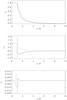Fig. 3 Dependence of the three velocity components of the eigenfunction with the radial coordinate. For this particular example, ρi/ρe = 3, p = 1/2, q = 3/2 and α = 0.01. The continuous and dashed lines correspond to the modes (m,k) and ( − m,k), while the dotted line represents the mode (m,k) in the absence of twist (α = 0).

We now aim to know the effect of twist on the eigenfunctions. It can be shown from the MHD equations (see Appendix A) that if Fourier analysis is performed in both the azimuthal and longitudinal direction, like in the present case, then there is a phase shift between the radial component (pure real function) and the azimuthal and longitudinal components (purely imaginary functions). In Fig. 3 the radial dependence of v_r, v_ϕ and v_z is plotted for the modes (m,k) (continuous line) and (−m,k) (dashed line). The same figure is obtained for the modes (−m, − k) and (m, − k). We see that the radial dependence of the modes is essentially the same inside the tube and only in the external medium near the tube boundary the dependence is slightly different (compare also with the dotted line, which represents the eigenfunction for the classical untwisted tube). The azimuthal velocity component shows more relevant differences for the two modes. The mode (m,k) has a reduced shear at the tube boundary while the opposite behaviour is displayed by the mode (−m,k), showing an increased shear with respect to the un-twisted case. This behaviour is also present in the v_z component, which is introduced by the presence of twist. Since we are in the zero-β approximation, the velocity along the magnetic field is zero, i.e., v_∥ = v·B₀/ | B₀ |  = 0, as expected. The v_z component has a jump at the tube boundary and is different from zero only in the region where there is twist (in this particular example between r = 1/2R and r = 3/2R). Notice that the amplitude of this velocity component is rather small in comparison with v_r and v_ϕ since we are considering a weak twist.

5. Results: standing waves

So far we focused on both azimuthally and longitudinally propagating waves. Our interest is now on the analysis of standing waves, if they exist in the twisted configuration.

5.1. Standing in ϕ, propagating in z

An azimuthally propagating wave, for example the mode m = 1, produces a motion that displaces the whole tube and its axis is moving following a circular path because of the propagating nature of the wave in ϕ. If the motion is clockwise for m then it is anti-clockwise for  − m. For the tube to oscillate transversally, the propagating m mode has to be combined with the  − m mode. When there is no twist, the frequency of the mode (m,k) is the same as the for the mode ( − m,k) (ω = kc_k in the thin tube limit), and the superposition is trivial. In the presence of twist the situation is more complicated since, as we have shown in Sect. 4, the modes (m,k) and (−m,k) have different frequencies. This means that with a single longitudinal wavenumber it is not possible to have a standing solution in the azimuthal direction. However, we have shown that we can always find another pair of wavenumbers with the same frequency. This means that the linear combination of the modes (m,k₁) and ( − m,k₂) will lead to the standing solution in ϕ we are looking for. Formally, we have to combine the two waves, $\begin{array}{ccc}\mathit{y}\mathrm{=}\mathit{f}\mathrm{\left(}\mathit{r}\mathrm{\right)}\exp \mathrm{i}\left(\mathit{\omega t}\mathrm{+}\mathit{m\varphi }\mathrm{+}{\mathit{k}}_{\mathrm{1}}\mathit{z}\right)\mathrm{+}\mathit{g}\mathrm{\left(}\mathit{r}\mathrm{\right)}\exp \mathrm{i}\left(\mathit{\omega t}\mathrm{-}\mathit{m\varphi }\mathrm{+}{\mathit{k}}_{\mathrm{2}}\mathit{z}\right)\mathit{,}& & \end{array}$(39)where y is, for example, any of the velocity components of the eigenfunction. Note that f(r) and g(r) are different functions since they are associated to different pairs of wavenumbers (m,k₁) and ( − m,k₂). However, in the thin tube approximation, when k₁R ≪ 1 and k₂R ≪ 1, the two functions are essentially the same (f(r) ≈ g(r) or f(r) ≈  − g(r) as Fig. 3 suggests). This is a nontrivial assumption, which might not be a good approximation when we relax the thin tube and the small α approximations. Using this approximation, Eq. (39) reduces to $\begin{array}{ccc}\mathit{y}\mathrm{=}\mathit{f}\mathrm{\left(}\mathit{r}\mathrm{\right)}\cos \left(\mathit{m\varphi }\mathrm{+}{\mathit{k}}_{\mathrm{T}}\mathit{z}\right)\exp \mathrm{i}\mathrm{(}\mathit{\omega t}\mathrm{+}\mathit{k}{\mathit{z}}^{\mathrm{)}}\mathit{,}& & \end{array}$(40)where we have introduced for convenience the following notation 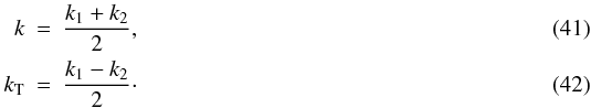$\begin{array}{ccc}\mathit{k}& \mathrm{=}& \\ {\mathit{k}}_{\mathrm{T}}& \mathrm{=}& \end{array}$If instead of the sum of the modes (m,k₁) and ( − m,k₂) we choose the difference as the linear combination, we find $\begin{array}{ccc}\mathit{y}\mathrm{=}\mathit{f}\mathrm{\left(}\mathit{r}\mathrm{\right)}\sin \left(\mathit{m\varphi }\mathrm{+}{\mathit{k}}_{\mathrm{T}}\mathit{z}\right)\exp \mathrm{i}\mathrm{(}\mathit{\omega t}\mathrm{+}\mathit{k}{\mathit{z}}^{\mathrm{)}}\mathit{.}& & \end{array}$(43)It is straightforward to construct the standing solution in ϕ but propagating in the positive z-direction (note that Eq. (40) represents a wave propagating in the negative z-direction). The solution is based on the superposition of the modes ( − m, − k₁) and (m, − k₂), and it is $\begin{array}{ccc}\mathit{y}\mathrm{=}\mathit{f}\mathrm{\left(}\mathit{r}\mathrm{\right)}\cos \left(\mathit{m\varphi }\mathrm{+}{\mathit{k}}_{\mathrm{T}}\mathit{z}\right)\exp \mathrm{i}\mathrm{(}\mathit{\omega t}\mathrm{-}\mathit{k}{\mathit{z}}^{\mathrm{)}}\mathit{.}& & \end{array}$(44)Again the sinus solution is obtained when we subtract the modes.

Equations (40) and (44) represent propagating waves in the z-direction and produce a transverse displacement of the tube so that now it depends on z through the term k_Tz. Thus, the direction of the transverse oscillation of the loop varies as the wave propagates along the tube. This represents a change in the polarisation of the transverse motion and is one of the main effects of twist on the eigenmodes. For the untwisted tube the polarisation of oscillation is always the same since k_T = 0.

The choice of k₁ and k₂ is not arbitrary since the modes with the pairs of wavenumbers (m,k₁) and ( − m,k₂) (the same applies to the combination ( − m, − k₁) and (m, − k₂)) need to have the same frequency. The appropriate wavenumbers can always be determined numerically for a given frequency, as Fig. 1 suggests. However, if α is small, this selection is straightforward because we can use the approximations for the frequency (see Eqs. (37), (38)) to calculate k₁ and k₂, 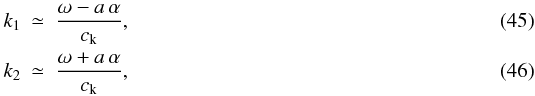$\begin{array}{ccc}{\mathit{k}}_{\mathrm{1}}& \mathrm{\simeq }& \frac{\mathit{\omega }\mathrm{-}\mathit{a}\hspace{0.17em}\mathit{\alpha }}{{\mathit{c}}_{\mathrm{k}}}\mathit{,}\\ {\mathit{k}}_{\mathrm{2}}& \mathrm{\simeq }& \frac{\mathit{\omega }\mathrm{+}\mathit{a}\hspace{0.17em}\mathit{\alpha }}{{\mathit{c}}_{\mathrm{k}}}\mathit{,}\end{array}$where a is the slope of the curves. Now using Eqs. (41) and (42) we have $\begin{array}{ccc}\mathit{k}& \mathrm{\simeq }& \frac{\mathit{\omega }}{{\mathit{c}}_{\mathrm{k}}}\mathit{,}\\ {\mathit{k}}_{\mathrm{T}}& \mathrm{\simeq }& \end{array}$From the first equation we conclude that the dispersion relation of the wave in the twisted case, ω = kc_k, is exactly the same as in the untwisted tube (under the thin-tube approximation and for weak twist). Thus, for weak twist, there is no effect on the frequency of the propagating waves in z and standing waves in ϕ. Nevertheless, from the second equation we find that the polarisation of the motion shows a dependence with twist (k_T ≠ 0). This dependence is linear with α. For the un-twisted case (α = 0) we recover the well-known solution of the transverse kink mode without variation of polarisation along the tube.

5.2. Standing in z, propagating in ϕ

Now we seek solutions that are standing in the z-direction. These solutions have to satisfy line-tying conditions, i.e., the three velocity components must be zero at the footpoints of the loop, located at z = 0 and z = L, where L is the total length of the tube. We proceed as in the previous section and select the appropriate superposition of modes. A suitable choice is (m,k₁) and (m, − k₂), $\begin{array}{ccc}\mathit{y}\mathrm{=}\mathit{f}\mathrm{\left(}\mathit{r}\mathrm{\right)}\left(\exp \mathrm{i}\left(\mathit{\omega t}\mathrm{+}\mathit{m\varphi }\mathrm{+}{\mathit{k}}_{\mathrm{1}}\mathit{z}\right)\mathrm{+}\exp \mathrm{i}\left(\mathit{\omega t}\mathrm{+}\mathit{m\varphi }\mathrm{-}{\mathit{k}}_{\mathrm{2}}\mathit{z}\right)\right)\mathit{,}& & \end{array}$(49)which can be written as $\begin{array}{ccc}\mathit{y}\mathrm{=}\mathit{f}\mathrm{\left(}\mathit{r}\mathrm{\right)}\cos \mathrm{(}\mathit{k}{\mathit{z}}^{\mathrm{)}}\exp \mathrm{i}\left(\mathit{\omega t}\mathrm{+}\mathit{m\varphi }\mathrm{+}{\mathit{k}}_{\mathrm{T}}\mathit{z}\right)\mathit{.}& & \end{array}$(50)The other choice corresponds to the modes ( − m, − k₁) and ( − m, + k₂), which represent a propagating wave in the positive ϕ-direction, $\begin{array}{ccc}\mathit{y}\mathrm{=}\mathit{f}\mathrm{\left(}\mathit{r}\mathrm{\right)}\cos \mathrm{(}\mathit{k}{\mathit{z}}^{\mathrm{)}}\exp \mathrm{i}\left(\mathit{\omega t}\mathrm{-}\mathit{m\varphi }\mathrm{-}{\mathit{k}}_{\mathrm{T}}\mathit{z}\right)\mathit{.}& & \end{array}$(51)As in the previous expressions, a sinus is obtained instead of a cosinus when the difference of the modes is considered instead of the sum, $\begin{array}{ccc}\mathit{y}\mathrm{=}\mathit{f}\mathrm{\left(}\mathit{r}\mathrm{\right)}\sin \mathrm{(}\mathit{k}{\mathit{z}}^{\mathrm{)}}\exp \mathrm{i}\left(\mathit{\omega t}\mathrm{+}\mathit{m\varphi }\mathrm{+}{\mathit{k}}_{\mathrm{T}}\mathit{z}\right)\mathit{,}& & \end{array}$(52)and $\begin{array}{ccc}\mathit{y}\mathrm{=}\mathit{f}\mathrm{\left(}\mathit{r}\mathrm{\right)}\sin \mathrm{(}\mathit{k}{\mathit{z}}^{\mathrm{)}}\exp \mathrm{i}\left(\mathit{\omega t}\mathrm{-}\mathit{m\varphi }\mathrm{-}{\mathit{k}}_{\mathrm{T}}\mathit{z}\right)\mathit{.}& & \end{array}$(53)Strictly speaking these modes cannot be classified as fully standing modes, because of the z dependence in the exponential.

Applying line-tying conditions imposes restrictions on the wavenumbers. Using the sinus solution given by Eq. (52) or (53) allows us to easily impose that the velocity must be zero z = 0 and z = L. The first condition is trivially satisfied while the second leads to $\begin{array}{ccc}\sin \mathrm{(}\mathit{k}{\mathit{L}}^{\mathrm{)}}\mathrm{=}\mathrm{0}\mathit{,}& & \end{array}$(54)and thus $\begin{array}{ccc}\mathit{k}\mathrm{=}\frac{\mathit{\pi }}{\mathit{L}}\mathit{n,n}\mathrm{=}\mathrm{1}\mathit{,}\mathrm{2}\mathit{,}\mathrm{3}\mathit{...}& & \end{array}$(55)This is essentially the same situation as in the untwisted tube, we have a discrete set of wavenumbers satisfying the boundary conditions.

In constructing the standing solution in z we have assumed that this solution is the superposition of two propagating waves with the same frequency, different longitudinal wavenumbers and the same radial dependence. As we have explained, this is only true within limit kR ≪ 1. In principle, we cannot assume a Fourier analysis in the z-direction because of line-tying conditions and consider single modes if we aim to obtain the full solution to the problem. For this reason, we now calculate the eigenmodes by solving the problem in r and z for a fixed m. This will allow us to compare the results with the semi-analytical results given by Eqs. (47) and (48). We used the two-dimensional version of the code PDE2D to calculate the modes with line-tying conditions at z = 0 and z = L. In Fig. 2 the eigenfrequency is plotted as a function of twist. Clearly, the frequency is almost independent of α (see the continuous horizontal line), which agrees with the analytical results obtained within the limit of small α given by Eq. (47) (compare also the continuous horizontal line with the dotted line, which corresponds to the untwisted case). Therefore, it is a good approximation (within the limit of small α) to assume that we can construct standing eigenmodes by summing two propagating waves with the same frequency but slightly different wavenumbers.

A plot of the eigenfunction at r = 0 and ϕ = 0 as a function of z is shown in Fig. 4. It is worth to mention that for the 2D problem the eigenfunction is always a complex number (this can be seen from Eqs. (A.1) − (A.6) in the Appendix) although the frequency is still a real magnitude since we do not consider unstable modes or resonances. For this reason we represent the modulus and the phase (δ) of the eigenfunction in Fig. 4. The modulus has a sinusoidal profile while the phase shows a linear dependence with z. This is exactly the behaviour predicted by Eq. (52). The slope of the phase is precisely the magnitude k_T, which is negative according to Eq. (48). The m =  −1 mode shows the expected positive slope, in agreement with Eqs. (53) and (48).

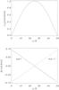Fig. 4 Eigenfunction as a function of z at the loop axis calculated numerically using line-tying conditions. The modulus and phase are plotted for the modes m =  ± 1.

5.3. Standing in ϕ and z

Once we have derived the solutions that are standing, or equivalent to standing, in one of the directions, it is straightforward to address the full standing problem. There are two ways to proceed that must be equivalent, either we add the solutions that are standing in ϕ but propagating in z, or we combine the solutions that are (almost) standing in z but propagating in ϕ. For example, from the combination of the solution given by Eq. (40), representing a standing wave in ϕ but propagating in z, minus the complementary wave travelling in the opposite z-direction given by Eq. (44), we find the “full” standing solution $\begin{array}{ccc}\mathit{y}\mathrm{=}\mathit{f}\mathrm{\left(}\mathit{r}\mathrm{\right)}\cos \left(\mathit{m\varphi }\mathrm{+}{\mathit{k}}_{\mathrm{T}}\mathit{z}\right)\sin \mathrm{(}\mathit{k}{\mathit{z}}^{\mathrm{)}}\exp \left(\mathrm{i}\mathit{\omega t}\right)\mathit{.}& & \end{array}$(56)It is easy to check that we obtain exactly the same expression by combining the solutions given in Eqs. (52), (53) for mainly representing standing waves in z but propagating in ϕ.

Based on Eq. (56) and using the proper phase shifts between the components of the displacement, we obtain the following eigenfunction $\begin{array}{ccc}{\mathit{\xi }}_{\mathit{r}}& \mathrm{=}& \\ {\mathit{\xi }}_{\mathit{\varphi }}& \mathrm{=}& \\ {\mathit{\xi }}_{\mathit{z}}& \mathrm{=}& \end{array}$Similar expressions have been used in the past as approximate solutions to test the stability of different twisted magnetic configurations. However, as far as we know, these expressions have not been applied to stable kink waves.

From Eqs. (57) − (59) we can easily calculate the displacement of the tube axis, which is a relevant quantity when it comes to observations of transverse loop waves. According to Fig. 3, inside the tube $\begin{array}{}{}_{\mathrm{˜}}\\ \mathit{f}\end{array}\mathrm{\left(}\mathit{r}\mathrm{\right)}\mathrm{\simeq }\begin{array}{}{}_{\mathrm{˜}}\\ \mathit{g}\end{array}\mathrm{\left(}\mathit{r}\mathrm{\right)}\mathrm{=}\mathrm{const}\mathit{.}$ in the thin-tube approximation, and the displacement in z has a node at the axis. Thus, in Cartesian coordinates at the axis (x = y = 0) $\begin{array}{ccc}{\mathit{\xi }}_{\mathit{x}}& \mathrm{=}& {\mathit{\xi }}_{\mathrm{0}}\cos \left({\mathit{k}}_{\mathrm{T}}\mathit{z}\mathrm{+}{\mathit{\varphi }}_{\mathrm{0}}\right)\sin \mathrm{(}\mathit{k}{\mathit{z}}^{\mathrm{)}}\sin \mathrm{(}\mathit{\omega }{\mathit{t}}^{\mathrm{)}}\mathit{,}\\ {\mathit{\xi }}_{\mathit{y}}& \mathrm{=}& {\mathit{\xi }}_{\mathrm{0}}\sin \left({\mathit{k}}_{\mathrm{T}}\mathit{z}\mathrm{+}{\mathit{\varphi }}_{\mathrm{0}}\right)\sin \mathrm{(}\mathit{k}{\mathit{z}}^{\mathrm{)}}\sin \mathrm{(}\mathit{\omega }{\mathit{t}}^{\mathrm{)}}\mathit{,}\\ {\mathit{\xi }}_{\mathit{z}}& \mathrm{=}& \mathrm{0}\mathit{,}\end{array}$ ξ₀ being an arbitrary amplitude and ϕ₀ an arbitrary phase. These expressions show that the tube does not move along the axis while the displacement in the plane perpendicular to the axis is given by the product of two sinusoidal terms, one involving a scale associated to the twist, k_T, and another related to the longitudinal wavenumber, k. At the axis $\begin{array}{ccc}\sqrt{{\mathit{\xi }}_{\mathit{x}}^{\mathrm{2}}\mathrm{+}{\mathit{\xi }}_{\mathit{y}}^{\mathrm{2}}\mathrm{+}{\mathit{\xi }}_{\mathit{z}}^{\mathrm{2}}}\mathrm{=}{\mathit{\xi }}_{\mathrm{0}}\sin \mathrm{(}\mathit{k}{\mathit{z}}^{\mathrm{)}}\sin \mathrm{(}\mathit{\omega }{\mathit{t}}^{\mathrm{)}}\mathit{,}& & \end{array}$(63)meaning that the total displacement is exactly the same as in the un-twisted case. The difference is in the components of the displacement which have a different weight depending on the position along the tube.

In Fig. 5 the displacement of the tube axis is plotted for a situation with moderate twist. Although the calculations in the previous sections were made using a very weak twist, we expect that for higher values of the B_ϕ component the motion of the axis is qualitatively the same. The differences in the polarisation of the motion with respect to the untwisted situation (see dotted line) are evident in this plot. The motion of the tube is even more clear in Fig. 6 where the displacement of the tube is represented in three-dimensions at two different times during the oscillation. We clearly see the departures from the purely sinusoidal displacement for the untwisted case. In the top panel of Fig. 6 the displacement is closer to the first longitudinal harmonic than to the fundamental mode. However, at later stages of the oscillation, see bottom panel of Fig. 6, the motion resembles the fundamental mode. Thus, twist can have a pronounced effect on the displacement of the tube axis during the oscillation.

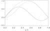Fig. 5 Displacement of the tube axis as a function of position along the twisted tube. The continuous line corresponds to the displacement in the x-direction while the dashed line represents the displacement in the y-direction. The dotted line is the purely sinusoidal displacement in the x-direction for the untwisted case. In this example, kT =  −0.75k, ϕ0 = 0, where ξ0/L = 1.

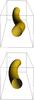Fig. 6 Snapshots of the displacement of the tube with twisted magnetic field at two different times during one oscillation period. In this example, kT =  −0.75k. The x-axis is horizonal, the y-axis is vertical and the z-axis is perpendicular to the xy-plane. Line-tying conditions are applied at the front and back planes (z = 0 and z = L).

6. Conclusions and discussion

From inspection of the local Alfvén frequency it might be anticipated that an azimuthal magnetic field can have a relevant effect on MHD waves even if  | B_ϕ |  ≪  | B_z | . It is the competition between the two quantities kR and α = B_ϕ,max/B_z(0) that determines the extent of the effect. In this work the quantity α is a small quantity by choice since we aim to focus on magnetic fields that are dominated by the longitudinal components. The quantity kR is often small as most of the loops are much longer than wide or the longitudinal wavelength is much longer that the radius of the loop. So it is really a competition between two small quantities kR and α. In the present investigation we have deliberately excluded the regime α/kR ~ 1 and focused our attention on α < α_J and α < α_M. In this way we avoid the interesting complications of resonant absorption. However, restricting ourselves to these values of α means that the azimuthal magnetic fields are in a sense very weak, and that the effects on the MHD waves by azimuthal magnetic field are less pronounced than they effectively are.

In general, the frequencies of MHD waves in models with nonconstant magnetic twist are nondegenerate compared to their counterparts in models with constant magnetic twist. This means that the frequencies of propagating waves with wavenumbers (m,k) and ( − m, − k) are equal but different from the frequency of the modes ( − m,k) and (m, − k). Twist breaks the symmetry with respect to the propagation direction. This property has consequences for standing modes that require the superposition of propagating waves. We have shown, using an approximate method valid for weak twist, that the frequency of standing waves is unaffected by the presence of twist. Under such conditions the tube oscillates transversally at the characteristic kink frequency.

However, the most interesting effect of magnetic twist on standing oscillations is in the change of polarisation of the transverse motion along the tube. We have analytically demonstrated that the change in the direction of the transverse displacement of the tube is linearly proportional to the twist. Moreover, the polarisation of the displacement of the axis along the tube is simply described by the product of two sinusoidal terms involving a wavenumber associated to the twist, and a longitudinal wavenumber that satisfies the line-tying boundary conditions at the footpoints of the loop (this is very similar to the situation for a tube with a siphon flow along the axis studied by Terradas et al. 2011). For a very weak twist, for instance 1/10 windings of the field along the loop axis, twist apparently introduces a motion perpendicular to the dominant direction of oscillation that is around nine times smaller in amplitude. The effect on the polarisation of the motion is small because the twist in the tube is very weak in this particular example. When the twist increases, the change in polarisation becomes stronger, as is shown in Figs. 5 and 6. An important result here is that a weak twist can produce displacements in any direction perpendicular to the unperturbed tube axis. Thus, in contrast to the effect of curvature of the magnetic field lines and the effect of nonuniform cross section, which both introduce vertical and horizontal modes, twist produces displacements in all directions. This agrees with the results of Ruderman & Scott (2011), who considered kink oscillation of a nonplanar coronal loop involving magnetic twist. In view of these results the role of twist on stable transverse motions has been underestimated in the context of loop oscillations. Potentially, the signatures of twist on standing transverse oscillations could be used as a way to infer the value of the azimuthal component of the magnetic field in coronal loops. This could have clear seismological applications. However, the fact that real coronal loops are in many cases nonplanar and noncircular, i.e., they have an helical shape (see the review of Aschwanden 2009), might complicate the comparison between theory and observations.

Finally, it is worth to notice that the analysis performed in this paper is based on the assumption of very weak twist. This has allowed us to avoid some complications that appear when the B_ϕ component of the magnetic field is increased. First of all, Alfvénic resonances cannot be avoided for moderate twist (see the work of Karami & Bahari 2010). Second, the modes might become kink-unstable. A detailed investigation of these effects on standing kink modes need to be addressed in future works.

Acknowledgments

J.T. acknowledges support from the Spanish Ministerio de Educación y Ciencia through a Ramón y Cajal grant. Funding provided under the project AYA2011-22846 by the Spanish MICINN and FEDER Funds, and the financial support from CAIB through the “Grups Competitius” scheme and FEDER Funds is also acknowledged by J.T. M.G. acknowledges financial support received during his visits at Universitat de les Illes Balears (UIB), funding under grant AYA2011-22846 and University of Leuven GOA 2009/009 is also acknowledged. The authors also thank J. Andries for his comments and suggestions during the preparation of this paper.

References

Appendix A: Appendix A

The ideal linearised MHD equations in the zero-β regime in the presence of magnetic twist are the following: 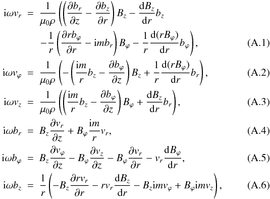$\begin{array}{ccc}\mathrm{i}\mathit{\omega }{\mathit{v}}_{\mathit{r}}& \mathrm{=}& \\ & & \\ \mathrm{i}\mathit{\omega }{\mathit{v}}_{\mathit{\varphi }}& \mathrm{=}& \frac{\mathrm{1}}{{\mathit{\mu }}_{\mathrm{0}}\mathit{\rho }}\left(\mathrm{-}\left(\frac{\mathrm{i}\mathit{m}}{\mathit{r}}{\mathit{b}}_{\mathit{z}}\mathrm{-}\frac{\mathit{\partial }{\mathit{b}}_{\mathit{\varphi }}}{\mathit{\partial z}}\right){\mathit{B}}_{\mathit{z}}\mathrm{+}\frac{\mathrm{1}}{\mathit{r}}\frac{\mathrm{d}\mathrm{\left(}\mathit{r}{\mathit{B}}_{\mathit{\varphi }}\mathrm{\right)}}{\mathrm{d}\mathit{r}}{\mathit{b}}_{\mathit{r}}\right)\mathit{,}\\ \mathrm{i}\mathit{\omega }{\mathit{v}}_{\mathit{z}}& \mathrm{=}& \frac{\mathrm{1}}{{\mathit{\mu }}_{\mathrm{0}}\mathit{\rho }}\left(\left(\frac{\mathrm{i}\mathit{m}}{\mathit{r}}{\mathit{b}}_{\mathit{z}}\mathrm{-}\frac{\mathit{\partial }{\mathit{b}}_{\mathit{\varphi }}}{\mathit{\partial z}}\right){\mathit{B}}_{\mathit{\varphi }}\mathrm{+}\frac{\mathrm{d}{\mathit{B}}_{\mathit{z}}}{\mathrm{d}\mathit{r}}{\mathit{b}}_{\mathit{r}}\right)\mathit{,}\\ \mathrm{i}\mathit{\omega }{\mathit{b}}_{\mathit{r}}& \mathrm{=}& {\mathit{B}}_{\mathit{z}}\frac{\mathit{\partial }{\mathit{v}}_{\mathit{r}}}{\mathit{\partial z}}\mathrm{+}{\mathit{B}}_{\mathit{\varphi }}\frac{\mathrm{i}\mathit{m}}{\mathit{r}}{\mathit{v}}_{\mathit{r}}\mathit{,}\\ \mathrm{i}\mathit{\omega }{\mathit{b}}_{\mathit{\varphi }}& \mathrm{=}& {\mathit{B}}_{\mathit{z}}\frac{\mathit{\partial }{\mathit{v}}_{\mathit{\varphi }}}{\mathit{\partial z}}\mathrm{-}{\mathit{B}}_{\mathit{\varphi }}\frac{\mathit{\partial }{\mathit{v}}_{\mathit{z}}}{\mathit{\partial z}}\mathrm{-}{\mathit{B}}_{\mathit{\varphi }}\frac{\mathit{\partial }{\mathit{v}}_{\mathit{r}}}{\mathit{\partial r}}\mathrm{-}{\mathit{v}}_{\mathit{r}}\frac{\mathrm{d}{\mathit{B}}_{\mathit{\varphi }}}{\mathrm{d}\mathit{r}}\mathit{,}\\ \mathrm{i}\mathit{\omega }{\mathit{b}}_{\mathit{z}}& \mathrm{=}& \end{array}$where v = (v_r,v_ϕ,v_z) is the velocity and b = (b_r,b_ϕ,b_z) is the perturbed magnetic field. If a Fourier analysis is performed in the z-direction, the derivatives with respect to z have to be replaced by ik.

All Figures

	Fig. 1 Frequency as a function of twist (α). The curves are obtained by solving the eigenvalue problem in 1D. The dotted line represents the solution for the untwisted case. For this particular example, ρi/ρe = 3, p = 1/2, q = 3/2. The two sets of solutions are associated to m = 1 and k1 = π/50R (thick lines), and k2 = π/48R (thin lines).
In the text

	Fig. 2 Frequency as a function of twist (α). For this particular example, ρi/ρe = 3, p = 1/2, q = 3/2 represented with thick lines while the case p = 0, q = 2 is plotted with thin lines. The dotted line represents the solution for the untwisted case. The horizontal continuous line is obtained by numerically solving the eigenvalue problem in 2D. The same notation as in Fig. 1 is used.
In the text

	Fig. 3 Dependence of the three velocity components of the eigenfunction with the radial coordinate. For this particular example, ρi/ρe = 3, p = 1/2, q = 3/2 and α = 0.01. The continuous and dashed lines correspond to the modes (m,k) and ( − m,k), while the dotted line represents the mode (m,k) in the absence of twist (α = 0).
In the text

	Fig. 4 Eigenfunction as a function of z at the loop axis calculated numerically using line-tying conditions. The modulus and phase are plotted for the modes m =  ± 1.
In the text

	Fig. 5 Displacement of the tube axis as a function of position along the twisted tube. The continuous line corresponds to the displacement in the x-direction while the dashed line represents the displacement in the y-direction. The dotted line is the purely sinusoidal displacement in the x-direction for the untwisted case. In this example, kT =  −0.75k, ϕ0 = 0, where ξ0/L = 1.
In the text

	Fig. 6 Snapshots of the displacement of the tube with twisted magnetic field at two different times during one oscillation period. In this example, kT =  −0.75k. The x-axis is horizonal, the y-axis is vertical and the z-axis is perpendicular to the xy-plane. Line-tying conditions are applied at the front and back planes (z = 0 and z = L).
In the text

References

- Aschwanden, M. J. 2009, Space Sci. Rev., 149, 31 [NASA ADS] [CrossRef] [Google Scholar]
- Aschwanden, M. J., & Schrijver, C. J. 2011, ApJ, 736, 102 [NASA ADS] [CrossRef] [Google Scholar]
- Aschwanden, M. J., Fletcher, L., Schrijver, C. J., & Alexander, D. 1999, ApJ, 520, 880 [NASA ADS] [CrossRef] [Google Scholar]
- Bennett, K., Roberts, B., & Narain, U. 1999, Sol. Phys., 185, 41 [NASA ADS] [CrossRef] [Google Scholar]
- Brown, D. S., Nightingale, R. W., Alexander, D., et al. 2003, Sol. Phys., 216, 79 [NASA ADS] [CrossRef] [Google Scholar]
- Carter, B. K., & Erdélyi, R. 2008, A&A, 481, 239 [NASA ADS] [CrossRef] [EDP Sciences] [Google Scholar]
- Díaz, A. J., Oliver, R., Ballester, J. L., & Soler, R. 2011, A&A, 533, A95 [NASA ADS] [CrossRef] [EDP Sciences] [Google Scholar]
- Einaudi, G., & van Hoven, G. 1983, Sol. Phys., 88, 163 [NASA ADS] [CrossRef] [Google Scholar]
- Erdélyi, R., & Carter, B. K. 2006, A&A, 455, 361 [NASA ADS] [CrossRef] [EDP Sciences] [Google Scholar]
- Erdélyi, R., & Fedun, V. 2006, Sol. Phys., 238, 41 [NASA ADS] [CrossRef] [Google Scholar]
- Erdélyi, R., & Fedun, V. 2007, Sol. Phys., 246, 101 [NASA ADS] [CrossRef] [Google Scholar]
- Erdélyi, R., & Fedun, V. 2010, Sol. Phys., 263, 63 [NASA ADS] [CrossRef] [Google Scholar]
- Giachetti, R., van Hoven, G., & Chiuderi, C. 1977, Sol. Phys., 55, 371 [NASA ADS] [CrossRef] [Google Scholar]
- Goossens, M., Hollweg, J. V., & Sakurai, T. 1992, Sol. Phys., 138, 233 [NASA ADS] [CrossRef] [Google Scholar]
- Hood, A. W., & Priest, E. R. 1979, Sol. Phys., 64, 303 [NASA ADS] [CrossRef] [Google Scholar]
- Hood, A. W., & Priest, E. R. 1981, Geophys. Astrophys. Fluid Dyn., 17, 297 [NASA ADS] [CrossRef] [Google Scholar]
- Hood, A. W., Priest, E. R., & Einaudi, G. 1982, Geophys. Astrophys. Fluid Dyn., 20, 247 [NASA ADS] [CrossRef] [Google Scholar]
- Hood, A. W., Archontis, V., Galsgaard, K., & Moreno-Insertis, F. 2009, A&A, 503, 999 [NASA ADS] [CrossRef] [EDP Sciences] [Google Scholar]
- Karami, K., & Bahari, K. 2010, Sol. Phys., 263, 87 [NASA ADS] [CrossRef] [Google Scholar]
- Kruskal, M. D., Johnson, J. L., Gottlieb, M. B., & Goldman, L. M. 1958, Phys. Fluids, 1, 421 [NASA ADS] [CrossRef] [Google Scholar]
- Moreno-Insertis, F., & Emonet, T. 1996, ApJ, 472, L53 [NASA ADS] [CrossRef] [Google Scholar]
- Nakariakov, V. M., Ofman, L., Deluca, E. E., Roberts, B., & Davila, J. M. 1999, Science, 285, 862 [NASA ADS] [CrossRef] [PubMed] [Google Scholar]
- Priest, E. R., Hood, A. W., & Anzer, U. 1989, ApJ, 344, 1010 [NASA ADS] [CrossRef] [Google Scholar]
- Raadu, M. A. 1972, Sol. Phys., 22, 425 [NASA ADS] [CrossRef] [Google Scholar]
- Ruderman, M. S. 2007, Sol. Phys., 246, 119 [NASA ADS] [CrossRef] [Google Scholar]
- Ruderman, M. S., & Erdélyi, R. 2009, Space Sci. Rev., 149, 199 [NASA ADS] [CrossRef] [Google Scholar]
- Ruderman, M. S., & Scott, A. 2011, A&A, 529, A33 [NASA ADS] [CrossRef] [EDP Sciences] [Google Scholar]
- Sewell, G. 2005, The Numerical Solution of Ordinary and Partial Differential Equations, 2nd edn. (Newark, NJ: Wiley) [Google Scholar]
- Shafranov, V. D. 1957, J. Nucl. Energy II, 5, 86 [Google Scholar]
- Suydam, B. R. 1958, Proc-1958-UN, 187 [Google Scholar]
- Terradas, J., Oliver, R., & Ballester, J. L. 2006, ApJ, 642, 533 [NASA ADS] [CrossRef] [Google Scholar]
- Terradas, J., Arregui, I., Verth, G., & Goossens, M. 2011, ApJ, 729, L22 [NASA ADS] [CrossRef] [Google Scholar]
- Vasheghani Farahani, S., Nakariakov, V. M., & van Doorsselaere, T. 2010, A&A, 517, A29 [NASA ADS] [CrossRef] [EDP Sciences] [Google Scholar]
- Velli, M., Hood, A. W., & Einaudi, G. 1990, ApJ, 350, 428 [NASA ADS] [CrossRef] [Google Scholar]
- Zaqarashvili, T. V., Díaz, A. J., Oliver, R., & Ballester, J. L. 2010, A&A, 516, A84 [NASA ADS] [CrossRef] [EDP Sciences] [Google Scholar]