| Issue |
A&A
Volume 548, December 2012
|
|
|---|---|---|
| Article Number | A67 | |
| Number of page(s) | 9 | |
| Section | Numerical methods and codes | |
| DOI | https://doi.org/10.1051/0004-6361/201219343 | |
| Published online | 22 November 2012 | |
A 3D radiative transfer framework
X. Arbitrary velocity fields in the comoving frame
1 Hamburger Sternwarte, Gojenbergsweg 112, 21029 Hamburg, Germany
e-mail: sknop@hs.uni-hamburg.de; yeti@hs.uni-hamburg.de
2 Homer L. Dodge Department of Physics and Astronomy, University of Oklahoma, 440 W Brooks, Rm 100, Norman, OK 73019, USA
e-mail: baron@ou.edu; bchen@ou.edu
3 Computational Research Division, Lawrence Berkeley National Laboratory, MS 50F-1650, 1 Cyclotron Rd, Berkeley, CA 94720, USA
e-mail: eabaron@lbl.gov
4 Physics Department, Univ. of California, Berkeley, CA 94720, USA
Received: 4 April 2012
Accepted: 20 October 2012
Aims. General 3D astrophysical atmospheres will have random velocity fields. We seek to combine the methods we have developed for solving the 1D problem with arbitrary flows to those that we have developed for solving the fully 3D relativistic radiative transfer problem for monotonic flows.
Methods. The methods developed for 3D atmospheres with monotonic flows, solving the fully relativistic problem along curves defined by an affine parameter, are very flexible and can be extended to the case of arbitrary velocity fields in 3D. Simultaneously, the techniques we developed for treating the 1D problem with arbitrary velocity fields are easily adapted to the 3D problem.
Results. The algorithm we present can be used to solve 3D radiative transfer problems that include arbitrary wavelength couplings. We use a quasi-analytic formal solution of the radiative transfer equation that significantly improves the overall computation speed. We show that the approximate lambda operator developed in previous work gives good convergence, even neglecting wavelength coupling. Ng acceleration also gives good results. We present tests that are of similar resolution to what has been presented using Monte-Carlo techniques, thus our methods will be applicable to problems outside of our test setup. Additional domain decomposition parallelization strategies will be explored in future work.
Key words: radiative transfer
© ESO, 2012
1. Introduction
In a series of papers (Hauschildt & Baron 2006, 2008, 2009, 2010; Baron & Hauschildt 2007; Baron et al. 2009b; Seelmann et al. 2010) we have developed a general framework for solving 3D radiative transfer problems in Cartesian, cylindrical, and spherical coordinates for both static and monotonic velocity fields in the comoving frame. We have also developed an Eulerian code for velocities  1000 km s-1 (Seelmann et al. 2010). The neglect of relativistic effects and resolution constraints limits the applicability of the Eulerian approach to v/c ≲ 0.01. Our affine method for solving the fully relativistic transfer equation is exact to all orders in v/c (Chen et al. 2007; Baron et al. 2009a). In a parallel series of papers we have introduced methods for solving the fully relativistic transfer equation in 1D spherical coordinates with arbitrary velocity fields (Baron & Hauschildt 2004; Knop et al. 2009a,b).
2. Basic formalism
Using the general formalism developed in Chen et al. (2007) we can derive the transfer equation in flat spacetime with arbitrary flows. We choose to work in spherical coordinates without loss of generality.
The photon’s four-momentum can be written  (1)where h is Planck’s constant, ξ is the affine parameter, λ∞ is the rest frame wavelength, and
  is the 3D direction of the photon as seen by a distant, stationary, observer. The four-velocity of the comoving observer in an arbitrary flow can be written
 ![\begin{equation} u^a=\gamma({\vec r},t)[1,\,\vec{\beta}({\vec r},t)], \end{equation}](/articles/aa/full_html/2012/12/aa19343-12/aa19343-12-eq9.png) (2)and the comoving wavelength λ can be obtained using
(2)and the comoving wavelength λ can be obtained using  (3)Here, β = v/c, and γ = (1 − β2) − 1/2, are the usual quantities of special relativity. The 3D geodesic in the flat spacetime can be parametrized as
  (4)where r0 is the starting point of the characteristics, and s is the rest frame physical distance related to the affine parameter ξ by
  (5)The radiative transfer equation can be written in terms of the affine parameter ξ as (see Eq. (10) of Chen et al. 2007):
  (6)where
  is the specific intensity measured by a comoving observer (note that Iλλ5 is observer-independent) at the (global) rest frame space-time point (r, t), toward the rest frame direction , and at the comoving wavelength λ. When expressing the 7D phase-space dependence of the comoving specific intensity, the only comoving variable we used was the wavelength λ, in particular, we did not use angles measured by a comoving observer to specify the direction of the photons. The advantages for this at first sight odd phase-space configuration have been explained in detail in Chen et al. (2007), and we applied this technique in Baron et al. (2009a).
We can rewrite Eq. (6) as ![\begin{eqnarray} \label{step2} \left.\frac{{\rm d}(ct)}{{\rm d}\xi}\frac{1}{c}\frac{\partial I_\lambda}{\partial t}\right|_\lambda + \frac{{\rm d}\vec{r}}{{\rm d}\xi}\cdot\nabla I_\lambda &+&\frac{{\rm d}\lambda}{{\rm d}\xi}\frac{\partial I_\lambda}{\partial \lambda}=\nonumber\\[2.5mm] && -\left(\chi_\lambda \frac{h}{\lambda}+\frac{5}{\lambda}\frac{{\rm d}\lambda}{{\rm d}\xi}\right)I_\lambda+\eta_\lambda \frac{h}{\lambda}, \end{eqnarray}](/articles/aa/full_html/2012/12/aa19343-12/aa19343-12-eq22.png) (7)or equivalently
(7)or equivalently ![\begin{eqnarray} \label{step3} \left.\frac{{\rm d}(ct)}{{\rm d}\xi}\frac{1}{c}\frac{\partial I_\lambda}{\partial t}\right|_\lambda &+& \frac{{\rm d}s}{{\rm d}\xi}\frac{{\rm d}\vec{r}}{{\rm d} s}\cdot\nabla I_\lambda +\frac{{\rm d}s}{{\rm d}\xi}\frac{{\rm d}\lambda}{{\rm d}s}\frac{\partial I_\lambda}{\partial \lambda}=\nonumber\\[2.5mm] && -\left(\chi_\lambda \frac{h}{\lambda}+\frac{5}{\lambda}\frac{{\rm d}s}{{\rm d}\xi}\frac{{\rm d}\lambda}{{\rm d}s}\right)I_\lambda+\eta_\lambda \frac{h}{\lambda}\cdot \end{eqnarray}](/articles/aa/full_html/2012/12/aa19343-12/aa19343-12-eq23.png) (8)Then using the definition of s from Eq. (5) and the fact that
(8)Then using the definition of s from Eq. (5) and the fact that  (9)we find
  (10)Equation (10) can be put into our standard form:
  (11)where
 ![\begin{equation} \label{fs} f(s)\equiv\frac{\lambda_\infty}{\lambda}=\gamma({\vec r},t)[1-{\hat{\vec n}}\cdot \vec{\beta}({\vec r},t)] \end{equation}](/articles/aa/full_html/2012/12/aa19343-12/aa19343-12-eq27.png) (12)is simply the Doppler factor, and
(12)is simply the Doppler factor, and  (13)Using Eqs. (4) and (12), a(s) is found to be
 ![\begin{equation} a(s)=\frac{1}{1-{\hat{\vec n}}\cdot\vec{\beta}}\left[\frac{{\rm d}}{{\rm d}s}({\hat {\vec n}}\cdot{\vec\beta})-\gamma^2\beta(1-{\hat{\vec n}}\cdot\vec{\beta})\frac{{\rm d}\beta}{{\rm d}s}\right], \end{equation}](/articles/aa/full_html/2012/12/aa19343-12/aa19343-12-eq30.png) (14)where β is the magnitude of β, and
(14)where β is the magnitude of β, and  (15)When we numerically integrate the radiation transfer equation, a(s) can be approximated as
  (16)where δs is the differential step size (physical distance) along the characteristics,
  and δβ are the changes of
  and β, respectively, when we move one step forward, which includes the changes induced by both time and spatial advances, for instance
  (17)Since few numerical schemes will be able to provide the fully implicit derivative, δβ, will often be obtained for example by the backward difference
  (18)In the stationary case, both β and f(s) are independent of time and specializing Eqs. (4) and (12) to that case, a(s) becomes
 ![\begin{eqnarray} a(s) &=&\frac{{\hat{\vec n}}\cdot\nabla({\hat{\vec n}}\cdot{\vec \beta})-\gamma^2\beta(1-{\hat{\vec n}}\cdot\vec{\beta})({ \hat{\vec n}}\cdot\nabla\beta)}{1-{\hat{\vec n}}\cdot{\vec \beta}} \nonumber \\[2mm] &=&-({\hat{\vec n}}\cdot\nabla) \ln (1-{\hat{\vec n}}\cdot{\vec\beta})-\gamma^2\beta({\hat{\vec n}}\cdot\nabla\beta), \label{eqn:adef} \end{eqnarray}](/articles/aa/full_html/2012/12/aa19343-12/aa19343-12-eq42.png) (19)where we have used the fact that along the characteristics, d/ds no longer contains the time derivative and is thus the directional derivative operator, that is, d/d
(19)where we have used the fact that along the characteristics, d/ds no longer contains the time derivative and is thus the directional derivative operator, that is, d/d . We recall that in the flat spacetime that we are considering, our characteristics are straight lines for all velocity flows.
In terms of its spherical components, β can be written  (20)where
  are the spherical orthonormal basis vectors at point r(r,θ,φ), i.e.
 ![\begin{eqnarray} \label{spherical-base} \hat{\vec e}_r&=&(\sin\theta\cos\phi, \sin\theta\sin\phi, \cos\theta),\nonumber\\[2mm] \hat{\vec e}_\theta&=&(\cos\theta\cos\phi,\cos\theta\sin\phi,-\sin\theta),\nonumber\\[2mm] {\hat{\vec e}}_{\phi}&=&(-\sin\phi,\cos\phi,0), \end{eqnarray}](/articles/aa/full_html/2012/12/aa19343-12/aa19343-12-eq47.png) (21)and consequently the
(21)and consequently the  in Eq. (16) can be calculated using
 ![\begin{eqnarray} \hat{\vec n}\cdot{\vec\beta}&=&\beta_r \hat{\vec n}\cdot\hat{\vec e}_r +\beta_{\theta}\hat{\vec n}\cdot \hat{\vec e}_{\theta}+\beta_{\phi} \hat{\vec n}\cdot\hat{\vec e}_{\phi}\nonumber\\[2mm] &\equiv& \beta_r n_r+\beta_{\theta} n_{\theta}+\beta_{\phi} n_{\phi} \end{eqnarray}](/articles/aa/full_html/2012/12/aa19343-12/aa19343-12-eq49.png) (22)(note that along the characteristics, has constant Cartesian components, nx, ny, nz, but changing spherical components, nr, nθ, nφ). Writing
(22)(note that along the characteristics, has constant Cartesian components, nx, ny, nz, but changing spherical components, nr, nθ, nφ). Writing  the spherical components nr, nθ,nφ can be easily computed using Eq. (21).
2.1. Comparison with Mihalas
At first glance, comparing Eq. (11) with Eq. (2.12) of Mihalas (1980) something seems amiss. Like Mihalas (1980), we work in the frame where spatial coordinates and clocks are measured by an observer at rest. However, Mihalas’ time derivative contains a Doppler factor, whereas ours does not. Also, our terms on the right-hand side contain Doppler factors, f(s), whereas those of Mihalas do not. The discrepency has been noted in passing by Chen et al. (2007) and arises because our s is a true distance measured in the observer’s frame, whereas that of Mihalas, sM, contains an extra Doppler factor:
 (note that f(s) is not a constant along the characteristics, and therefore sM is not related to the physical distance s by a simple affine transformation). Thus, we can transform from s to sM in Eq. (10) to find
 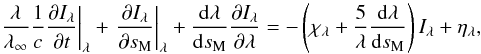 (23)which is very similar to the equation of Mihalas, except that the coefficient multiplying the time derivative term is the inverse Doppler factor f(s)-1, since we are working with Iλ instead of Iν, as did Mihalas. Jack et al. (2009) accidentally forgot to convert the time derivative from Iν to Iλ and thus their Eqs. (24), (25) have a coefficient of the time derivative with the Doppler factor in the numerator, rather than in the denominator. Thus, the time derivative terms in their Eqs. (24), (25) should be multiplied by f(s)-2 to give the correct equations.
2.2. Nonmonotonic flows
We are now in a position to tie together the work of Baron & Hauschildt (2004), Knop et al. (2009a) and Baron et al. (2009b). The formal solution in the monotonic case is an initial value problem in wavelength, but in the arbitrary flow case both spatial coordinates and wavelengths are fully coupled. This poses a significant memory cost, since the matrix obtained by finite-differencing the equations now contains every wavelength and not just the spatial points along the characteristic. The computational cost is surprisingly low because the linear system can be solved using the semi-analytic method of Knop et al. (2009a). While the framework that was given in Baron & Hauschildt (2004) and Baron et al. (2009b) was formulated for just one wavelength discretization, we included here the fully implicit discretization developed in Hauschildt & Baron (2004). Furthermore, we used the new formal solution that avoids negative generalized opacities (Knop et al. 2009b).
The stationary equation of radiative transfer in its characteristic form for the specific intensity I along a path s reads 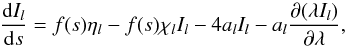 (24)where η is the emissivity, χ the opacity, and the subscript l indicates dependence on wavelength. The
  -term is the coupling term between the wavelengths and depends on the structure of the atmosphere and on the mechanism of the coupling (Mihalas 1980).
The wavelength derivative can be discretized in two ways as described in Hauschildt & Baron (2004). The different discretizations can be mixed via a Crank-Nicholson-like scheme with a mixing parameter ξ ∈ [ 0,1 ] . The wavelength discretized equation of radiative transfer can then be written as ![\begin{eqnarray} \label{eq:eqrt2} \frac{\mathrm{d} I_l}{\mathrm{d} s} &=& f(s)\eta_l - f(s)\chi_l I_l - a_l \left(4 + \xi \; p_l^| \right) I_l \nonumber \\ &{}& \; - \xi \; a_l \left( p_l^- I_{{l-1}} + p_l^+ I_{{l+1}} \right) \nonumber \\ &{}& \; - [1 - \xi] \; a_l \left( p_l^- I_{{l-1}} + p_l^| I_l + p_l^+ I_{{l+1}} \right), \end{eqnarray}](/articles/aa/full_html/2012/12/aa19343-12/aa19343-12-eq68.png) (25)where the
(25)where the  coefficients in an ordered wavelength grid λl − 1 < λl < λl + 1 are defined as
 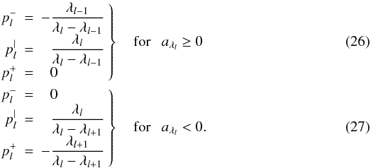 The dependence on the sign of aλ is introduced to define local upwind schemes (see Baron & Hauschildt 2004).
After introducing a generalized opacity (see Knop et al. 2009a,b) 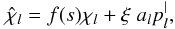 (28)defining the source functions
 ![\begin{eqnarray} S_l & = & \frac{\eta_l}{\chi_l} \\ \hat{S}_l & = & \frac{\chi_l}{\hat{\chi}_l} \Bigg\{ f(s) S_l - \xi \; \frac{a_l}{\chi_l} \left( p_l^- I_{{l-1}} + p_l^+ I_{{l+1}} \right) \Bigg\} \label{eq:srchat} \\ \tilde{S}_l & = & -\, \frac{a_l}{\hat{\chi}_l} \Bigg\{ [1 - \xi] \; \left( p_l^- I_{{l-1}} + p_l^+ I_{{l+1}}\right) + \left( 4 + [1 - \xi] \; p_l^| \right) I_l \Bigg\}, \label{eq:srctilde} \end{eqnarray}](/articles/aa/full_html/2012/12/aa19343-12/aa19343-12-eq74.png) a formal solution of the radiative transfer problem can be formulated. We used a full characteristic method throughout the atmosphere. The spatial position on a characteristic is then discretized on a spatial grid. In the following a pair of subscript indices will mark the position in the spatial grid and in the wavelength grid. Commonly the spatial grid is mapped locally onto an optical depth grid via the relation
a formal solution of the radiative transfer problem can be formulated. We used a full characteristic method throughout the atmosphere. The spatial position on a characteristic is then discretized on a spatial grid. In the following a pair of subscript indices will mark the position in the spatial grid and in the wavelength grid. Commonly the spatial grid is mapped locally onto an optical depth grid via the relation  . The formal solution of the radiative transfer Eq. (25) between two points si − 1 and si on a spatial grid along the photon path can be written in terms of the optical depth as follows:
 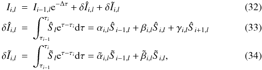 with Δτ = τi + 1,l − τi,l and
  . The α-β-γ coefficients are described in Olson & Kunasz (1987) and Hauschildt (1992).
  in Eq. (34) is linearly interpolated and in general different from the coefficients in Eq. (33) and is therefore marked with a tilde.
Equation (32) can be written in matrix notation for any given characteristic:  (35)Here I is a vector with all intensities, A is a square matrix that describes the influence of the different intensities upon each other, and ΔI is a vector with the thermal emission and scattering contribution of the source function. For a characteristic with ni spatial points and nl points in the wavelength grid, the intensity vector I has ni × nl entries. In the following a superscript of k will label the characteristic at hand. The components of the matrix A from Eq. (35) at the spatial point i and the wavelength point l are given by
 ![\begin{eqnarray} A^{\mathrm{-},k}_{i,l} & = & - \left( \xi \alpha^k_{i,l} + [1 - \xi] \, \tilde{\alpha}^k_{i,l} \right) \frac{a^k_{i-1,l}}{\hat{\chi}^k_{i-1,l}} p^{-,k}_{i-1,l} \label{eq:matrix_coeff_start} \\ B^{\mathrm{-},k}_{i,l} & = & - \left( \xi \beta^k_{i,l} + [1 - \xi] \, \tilde{\beta}^k_{i,l} \right) \frac{a^k_{i,l }}{\hat{\chi}^k_{i,l }} p^{-,k}_{i,l} \\ C^{\mathrm{-},k}_{i,l} & = &- \xi \gamma^k_{i,l} \frac{a^k_{i+1,l}}{\hat{\chi}^k_{i+1,l}} p^{-,k}_{i+1,l}\\ A^{\mathrm{\diagdown},k}_{i,l} & = & \! \! \exp{(-\Delta \tau^k_{i-1,l})} - \tilde{\alpha}^k_{i,l} \frac{a^k_{i-1,l}}{\hat{\chi}^k_{i-1,l}} \left[ 4 + [1\!-\! \xi] p^{|,k}_{i-1,l} \right] \\ B^{\mathrm{\diagdown},k}_{i,l} & = &- \tilde{\beta}^k_{i,l} \frac{a^k_{i,l}}{\hat{\chi}^k_{i,l}} \left[ 4 + [1 - \xi] \, p^{|,k}_{i,l} \right]\\ C^{\mathrm{\diagdown},k}_{i,l} & = & 0 \\ A^{\mathrm{+},k}_{i,l} & = &- \left( \xi \alpha^k_{i,l} + [1 - \xi] \, \tilde{\alpha}^k_{i,l} \right) \frac{a^k_{i-1,l}}{\hat{\chi}^k_{i-1,l}} p^{+,k}_{i-1,l} \label{eq:matrix_super1} \\ B^{\mathrm{+},k}_{i,l} & = &- \left( \xi \beta^k_{i,l} + [1 - \xi] \, \tilde{\beta}^k_{i,l} \right) \frac{a^k_{i,l }}{\hat{\chi}^k_{i,l }} p^{+,k}_{i,l} \label{eq:matrix_super2} \\ C^{\mathrm{+},k}_{i,l} & = &- \xi \gamma^k_{i,l} \frac{a^k_{i+1,l}}{\hat{\chi}^k_{i+1,l}} p^{+,k}_{i+1,l}. \label{eq:matrix_coeff_end} \end{eqnarray}](/articles/aa/full_html/2012/12/aa19343-12/aa19343-12-eq94.png) Following Knop et al. (2009a), the naming scheme of the quantities in Eqs. (36)–(44) indicates with which specific intensity element they are associated. For an index pair i and l a • − superscript refers to an intensity at wavelength l − 1, a •∖ superscript to the same wavelength, and • + to the next wavelength point l + 1. The A,B,C terms refer to the spatial points i − 1,i,i + 1, respectively. Equations (25)–(44) are nearly identical to those of Knop et al. (2009a) except for the explicit Doppler factor f(s), which arises because the photon direction is measured by a distant stationary observer here rather than by a comoving observer, as was the case in Knop et al. (2009a). We also clarified a problem with
Following Knop et al. (2009a), the naming scheme of the quantities in Eqs. (36)–(44) indicates with which specific intensity element they are associated. For an index pair i and l a • − superscript refers to an intensity at wavelength l − 1, a •∖ superscript to the same wavelength, and • + to the next wavelength point l + 1. The A,B,C terms refer to the spatial points i − 1,i,i + 1, respectively. Equations (25)–(44) are nearly identical to those of Knop et al. (2009a) except for the explicit Doppler factor f(s), which arises because the photon direction is measured by a distant stationary observer here rather than by a comoving observer, as was the case in Knop et al. (2009a). We also clarified a problem with  that was confusing in Knop et al. (2009a). The formal solution matrix is therefore identical in form to that shown in Fig. 1 of Knop et al. (2009a).
An element of the source function vector ΔI is given by (Knop et al. 2009a)  (45)Note that all Doppler factors are explicitlyhandled by including them in the opacity as χl ∗ f(s).
From Eq. (35) the solution for the specific intensity for a given spatial point and wavelength reads  (46)
(46)
2.2.1. The operator splitting method
Now that we have the formal solution, the full scattering problem can be solved by using operator splitting. The mean intensity Jλ is obtained from the source function Sλ by a formal solution of the radiative transfer equation, which is symbolically written using the Λ-operator Λλ as  (47)For the transition of a two-level atom, we have
  (48)where
  ,
,  with the normalized line profile φ(λ).
The Λ-iteration method, i.e. solving Eq. (48) by a fixed-point iteration scheme of the form  (49)fails in the case of high optical depths and small ϵ. This is because the largest eigenvalue of the amplification matrix (for Doppler-profiles) is approximately λmax ≈ (1 − ϵ)(1 − T-1), where T is the optical thickness of the medium (Mihalas et al. 1975). For small ϵ and high T, this is very close to unity and, therefore, the convergence rate of the Λ-iteration is very poor. A physical description of this effect can be found in Mihalas (1980).
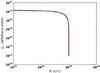 |
Fig. 1 Comparison of monotonic flow case with spherical symmetry solved using the full arbitrary velocity field method (red) to the well-tested 1D solution (black). The comoving mean intensity is plotted at each point in the computational volume. The agreement is at the 1% level. |
The idea of the ALI or operator splitting method is to reduce the eigenvalues of the amplification matrix in the iteration scheme (Cannon 1973) by introducing an approximate  -operator (ALO) Λ∗ and to split according to
  (50)and rewrite Eq. (48) as
  (51)This relation can be written as (Hamann 1987)
 ![\begin{equation} \left[1-\lstar(1-\e)\right]\Jnew = \Jfs - \lstar(1-\e)\Jold, \label{alo1} \end{equation}](/articles/aa/full_html/2012/12/aa19343-12/aa19343-12-eq123.png) (52)where
(52)where  . Equation (52) is solved to obtain the new values of
  , which are then used to compute the new source function for the next iteration cycle.
Mathematically, the ALI method belongs to the same family of iterative methods as the Jacobi or the Gauss-Seidel methods (Golub & Van Loan 1989). These methods have the general form  (53)for the iterative solution of a linear system Ax = b where the system matrix A is split according to A = M − N. For the ALI method we have M = 1 − Λ∗(1 − ϵ) and, accordingly,
  for the system matrix
  . The convergence of the iterations depends on the spectral radius, ρ(G), of the iteration matrix G = M-1N. For convergence the condition ρ(G) < 1 must be fulfilled, this puts a restriction on the choice of Λ∗. In general, the iterations will converge faster for a smaller spectral radius. To achieve a significant improvement compared to the Λ-iteration, the operator Λ∗ is constructed so that the eigenvalues of the iteration matrix G are much less than unity, resulting in swift convergence. Using parts of the exact matrix (e.g., its diagonal or a tri-diagonal form) will optimally reduce the eigenvalues of the G. The calculation and the structure of Λ∗ should be simple to make the construction of the linear system in Eq. (52) fast. For example, the choice
  is best in view of the convergence rate (it is equivalent to a direct solution by matrix inversion) but the explicit construction of is more time-consuming than the construction of a simpler Λ∗.
In the following discussion we use the notation of Hauschildt (1992) and Hauschildt & Baron (2006). The basic framework and the methods used for the formal solution and the solution of the scattering problem via operator splitting are discussed in detail in Hauschildt & Baron (2006) and will therefore not be repeated here. We have extended the framework to solve line transfer problems with a background continuum. The basic approach is similar to that of Hauschildt (1993). In the simple case of a two-level atom with background continuum that we consider here as a test case, we use a wavelength grid that covers the profile of the line including the surrounding continuum. We then use the wavelength-dependent mean intensities Jλ and approximate Λ operators Λ∗ to compute the profile-integrated line mean intensities and  via
via
 and are then used to compute an updated value for and the line source function
 where ϵ is the line thermalization parameter (0 for a purely absorptive line, 1 for a purely scattering line). B is the Planck function, Bλ, profile averaged over the line
 via the standard iteration method
 ![\begin{equation} \left[1-\lstar(1-\e)\right]\Jnew = \Jfs - \lstar(1-\e)\Jold, \label{alo2} \end{equation}](/articles/aa/full_html/2012/12/aa19343-12/aa19343-12-eq148.png) (54)where
(54)where  . This equation is solved directly to obtain the new values of , which are then used to compute the new source function for the next iteration cycle.
We construct the line directly from the wavelength-dependent Λ∗ generated by the solution of the continuum transfer problems.
Given the form of Eq. (46) for the formal solution, the construction of the Λ∗-operator can proceed exactly as described in Baron & Hauschildt (2004). However, to conserve memory, we have implemented the Λ∗-operator, retaining the spatial off-diagonal terms, but neglecting the off-diagonal terms in wavelength. We still find good convergence at considerable savings in memory (see below).
3. Test calculations
In this section we present the results of test calculations we performed to test the new algorithm in terms of accuracy by regression testing. We compare these to results of the homologous case (Baron et al. 2009b), and to the spherical nonmonotonic cases (Baron & Hauschildt 2004).
The test calculations were performed on Opteron CPUs running Linux (Franklin and Hopper at NERSC), on Intel CPUs (Carver at NERSC, ICE2 at HLRN, and our own local Xserve clusters), and on IBM CPUs (PWR-4 and PWR-5). The code was compiled with Gfortran/gcc/g++, ifort/icc/icpc (versions 11 and 12), and xlf/xlc/xlC and with NAG f95/gcc/g++. Using the varied compiler suites and CPUs allowed us to find numerous errors.
3.1. Regression with monotonic case
Figure 1 shows the profile of the mean intensity J for homologous flow and spherical symmetry. The test problem is similar to that of Baron et al. (2009b). These are the basic model parameters:
-
1.
An inner radius Rin = 1011 cm and an outer radius Rout = 1.01 × 1013 cm.
-
2.
A minimum optical depth in the continuum
 and a maximum optical depth in the continuum
  .
. -
3.
A gray temperature structure with K. That is the temperature solution of the spherical gray atmosphere problem with effective temperature (Mihalas 1978).
-
4.
An outer boundary condition
 and an inner boundary condition Iλ = Bλ for all wavelengths.
 -
5.
For the initial wavelength the boundary condition is taken from that given by the 3D homologous calculation for homologous tests and set equal to the Planck function Bλinit for non-homologous tests.
-
6.
A continuum extinction χc = C/r2, with the constant C fixed by the radius and optical depth grids.
-
7.
A parametrized coherent and isotropic continuum scattering given by
with 0 ≤ ϵc ≤ 1. κc and σc are the continuum absorption and scattering coefficients. In this work we have neglected scattering in the continuum.
The line of the simple two-level model atom is parameterized by the ratio of the profile-averaged line opacity χl to the continuum opacity χc and the line thermalization parameter ϵl. For the test cases presented below, we used ϵc = 1 and the line strength is given by Γ ≡ χl/χc = 102 to simulate a strong line, with varying ϵl (see below).
The test model is just an optically thick sphere put into the 3D grid. The velocity at the outer radius was set to be relativistic, vmax = 8 × 10⁴ km s-1. The calculation was performed on a spherical grid with 333 spatial points, 332 solid angle directions, and 22 wavelength points. This and all calculations presented below were parallelized over characteristics and were run on parallel clusters. Ng (Ng 1974; Auer 1987) acceleration was used to significantly speed up the operator splitting iterations for cases with scattering. Figure 2 shows the line profile at the surface, here we compare the 3D monotonic calculation (Baron et al. 2007) to the same calculation using the 3D arbitrary velocity algorithm. Because of the spatial resolution and the way that characteristics end at different points in a voxel (as opposed to always ending on a radial grid point in the 1D case), it is better to compare 3D cases to 3D cases.
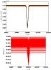 |
Fig. 2 Comparison of monotonic flow case with spherical symmetry solved using the full arbitrary velocity field method (green) to the 3D monotonic flow solution (red). The comoving mean intensity is plotted at the surface of the sphere. The test cases are identical, vmax = 8 × 10⁴ km s-1, 129 × 17 × 17 spatial voxels, 114 wavelength points, and 256 × 256 directions. The thermalization parameter in the line is ϵ = 10-3 and the line strength is Γ = 100. The lower panel shows the relative difference, δJλ/Jλ, as a function of wavelength. |
Figure 3 shows the convergence rate of a monotonic flow case, with ϵ = 10-4, with and without Ng accleration. Not only does Ng acceleration clearly improve the convergence rate, it gives almost the exact same errors as the same test setup using both the 3D and 1D homologous algorithms.
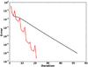 |
Fig. 3 Comparison of the convergence rate of a monotonic flow case with spherical symmetry with the thermalization parameter ϵ = 10-4 with and without Ng acceleration. The Ng acceleration is identical to that produced by the pure homologous 3D module. |
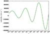 |
Fig. 4 Velocity profile used for the nonmonotonic velocity test with a damped sine wave. |
3.2. Sine velocity flow
Here we again consider a spherically symmetric case with the same physical parameters as in Sect. 3.1, but the velocity, while still radial is now given modulated by a damped sine wave. We have also introduced a line into the opacity with thermalization parameter ϵl = 1. The thermalization parameter in the continuum is ϵc = 1. This case was calculated in 1D in Baron & Hauschildt (2004). Figure 4 shows the velocity as a function of radial optical depth in the continuum. The spatial grid was 129 × 65 × 17 and the solid angle resolution was set to 5122. The maximum velocity is v ≈ 10 000 km s-1 and the total number of wavelength points is 226. Figure 5 shows the comoving mean intensity Jλ from each surface voxel as a function of wavelength λ. The 1D result is plotted (the green curve) and the agreement is good to the sub-percent level. The variation in the velocity leads to an asymmetric line profile even in the comoving frame. But since this test has such a high spatial resolution, it requires a significant amount of memory per process. We explored the effects of lower spatial resolution, 129 × 17 × 17, while keeping the high solid angle resolution 512 × 512. Figure 6 shows the mean intensity as a function of wavelength for the outmost part of the sphere. For computational expediency we set the line thermalization parameter ϵl = 1. The spread in the results of 1.5% is indicative of the accuracy of these calculations, whereas the deviation of the envelope of the solution is indicative of the low spatial resolution of this calculation. While modern nodes may have 24 CPUs, but only about 1 GB of RAM per CPU, it is unfortunate that the evelope of the low spatial resolution calculation is offset from the 1D result. This shows that not only solid angle resolution is important, but spatial resolution is quite important as well. Figure 7 shows the same calculation with the spatial grid enhanced to 129 × 65 × 65 and the solid angle grid reduced to 32 × 24 (Hauschildt & Baron 2010). As can be seen in Fig. 7, the reduced solid angle resolution increases the spread by roughly a factor of two, but now the 3D solution envelopes the 1D nonmonotonic result. With this higher spatial resolution, the spread can be further reduced by increasing the solid angle resolution, which shows near-perfect weak scaling, and thus does not increase the wallclock time required for these calculations (although it does require more CPUs).
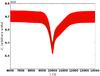 |
Fig. 5 Line profile for the damped sine-wave velocity case with high spatial nr = 129, nθ = 65, and nφ = 17, and angular resolution nΩ = 512 × 512. The comoving mean intensity Jλ for each voxel on the surface (there are 65 × 17 = 1105 of them) is plotted as a function of λ (red lines). The green curve is the 1D result using the methods of Baron & Hauschildt (2004) and Knop et al. (2009b,a). Here the scattering fraction is ϵ = 10-4 and the line strength is Γ = 100. |
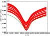 |
Fig. 6 Line profile for the damped sine-wave velocity case with lower spatial nr = 129, nθ = 17, and nφ = 17, and higher angular resolution nΩ = 512 × 512 than in Fig. 5. The comoving mean intensity Jλ for each voxel on the surface (there are 65 × 17 = 1105 of them) is plotted as a function of λ (red lines). The green curve is the 1D result using the methods of Baron & Hauschildt (2004) and Knop et al. (2009b,a). Here the scattering fraction is ϵ = 1 for computational expediency, and the line strength is Γ = 100. With the very low spatial resolution, the 3D result no longer envelopes the 1D result (which by assuming spatial spherical symmetry has essentially infinite resolution in nθ, and nφ). |
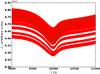 |
Fig. 7 Line profile for the damped sine-wave velocity case with higher spatial resolution, but lower angular resolution than in Fig. 5. The spatial resolution is nr = 129, nθ = 65, and nφ = 65, and the angular resolution is reduced to nΩ = 32 × 24. The comoving mean intensity Jλ for each voxel on the surface (there are 65 × 17 = 1105 of them) is plotted as a function of λ (red lines). The green curve is the 1D result using the methods of Baron & Hauschildt (2004) and Knop et al. (2009b,a). Here the scattering fraction is ϵ = 1 for computational expediency, and the line strength is Γ = 100. |
3.3. Example of radial nonhomologous flows
The previous tests were all totally spherically symmetric, with radial variations in the velocity field. We now assume the flow to be radial and azimuthally symmetric, i.e.  (56)For this case, we have
  and
and ![\begin{equation} \hat{\vec n}\cdot\nabla(\hat{\vec n}\cdot\vec{\beta})=\frac{1}{r}\left[p'qn_rn_\theta+p\left(q'r\right)n_r^2+pq\left(1-n_r^2\right)\right], \label{eqn:nr_nhatdotgradnhatdotbeta} \end{equation}](/articles/aa/full_html/2012/12/aa19343-12/aa19343-12-eq204.png) (59)where we made use of
(59)where we made use of  (60)and
  (61)Here an over dot implies
  e.g.,
e.g.,  etc., and a prime denotes differentiation with respect to μ = cosθ.
Inserting Eqs. (57)–(59) into Eq. (19), we find an analytic expression for a(s): ![\begin{eqnarray} a(s)&=&\frac{p'qn_rn_\theta+p(q'r)n_r^2+pq(1-n_r^2)}{r(1-p q n_r)}\nonumber\\ &&\qquad -\gamma^2 pq \left[pn_rq'(r)+\frac{1}{r}p'(\theta)q n_\theta \right], \end{eqnarray}](/articles/aa/full_html/2012/12/aa19343-12/aa19343-12-eq210.png) (62)where the spherical components of the unit vector
(62)where the spherical components of the unit vector  are
are  (63)For p(θ), we use an expansion in terms of Legendre polynomials (which form a complete and orthonormal basis for axially symmetric spherical functions)
  (64)with
 and
and  etc., where μ = cosθ. We consequently obtain
  (65)with
  and
and  etc. (note that the case
  degenerates to homologous flow). We can use this finite expansion in terms of the Legendre polynomial
  to construct azimuthally symmetric jets.
As a simple example of nonspherically symmetric flow, we run a test case where  (66)i.e. we take q(r) = c0r (c0 is a constant), which simplifies a(s) to be
 ![\begin{equation} a(s)=c_0\left[\frac{p+p'n_rn_\theta}{1-rn_rp}-\gamma^2\beta(pn_r+p'n_\theta)\right]. \end{equation}](/articles/aa/full_html/2012/12/aa19343-12/aa19343-12-eq227.png) (67)Furthermore, we assume
(67)Furthermore, we assume  (68)i.e., we perturb the homologous flow by adding a second-order Legendre polynomial with perturbation coefficient 0.5. We show the resulting mean intensity plot J(θ,φ) at the boundary R = Rout in Fig. 8. We obtained perfect azimuthal symmetry as expected from the form of β in Eq. (66), although it was not explicitly enforced. Furthermore, we also recovered the symmetry with respect to the north/south pole (i.e., symmetry under a reflection with respect to the equatorial plane, θ → π − θ), which is characteristic for Legendre polynomials of even order, see Eq. (68). Figure 9 shows a longitudinal slice of the comoving intensity, which shows that the comoving mean intensity varies by roughly a factor of ten from the pole to the equator. This is just due to the effect that the continuum level varies with the maximum velocity (Baron et al. 2009b).
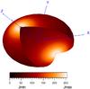 |
Fig. 8 Comoving mean intensity J(θ,φ) plotted at the surface R = Rout for case where |


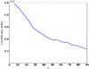 |
Fig. 9 Comoving mean intensity J(θ,φ0) plotted at the surface R = Rout for a fixed (arbitrarily chosen) value of φ = φ0. The variation of nearly an order of magnitude from the pole to the equator is due to the fact the the continuum level is a function of the velocity. |
3.4. Checkpointing
We implemented a checkpointing scheme that allows for restarts and new starts with higher resolution in solid angle. We simply write out (using stream I/O) the Λ∗ operator once it has been calculated, and the value of J at each voxel after each ALO iteration. Since these calculations require significant numbers of processors, which may go down, or calculations may run out of time, this allows us to perform perfect restarts. We checked that restarting from the checkpoint files works perfectly and that the calculations are converged in a single iteration when restarting from a converged checkpoint file. We write Λ∗ and J to separate files, since that allows us to read just J, and then recalculate Λ∗ if we restart with a higher resolution. We checked this, and it allows us to use a low-resolution calculation (performed on fewer processors, for example) and then converge the higher resolution calculation with roughly half as many iterations for each resolution increase. Table 1 shows the rate of convergence for a test with homologous velocity fields (chosen for computational expedience), vmax = 105 km s-1 and ϵ = 10-5. While the restart result still requires several iterations, this scheme allows for some speedup. The small ϵ and high maximum velocity make this test particularly demanding. The calculations were all restarted such that Ng acceleration cannot begin until the fourth iteration, and thus the restart calculations converge more slowly than they could. The scheme could indeed possibly be made more efficient by keeping the previous three values of , so that the restart iteration could immediately use Ng accleration.
Convergence rate for homologous test with vmax = 105 km s-1 and ϵ = 10-5, starting from the previous test.
4. Conclusion
We presented algorithm strategies and details for the solution of the radiative transfer problem in 3D atmospheres with arbitrary wavelength couplings.
Future possible applications are the velocity profiles of cool stellar winds, treating partial redistribution, calculating radiative transfer in shock fronts like in accretion shocks, calculating quasar jets, and general relativistic situations such as a rotating black hole.
Acknowledgments
This work was supported in part by SFB 676, GRK 1354 from the DFG, NSF grant AST-0707704, and US DOE Grant DE-FG02-07ER41517. Support for Program number HST-GO-12298.05-A was provided by NASA through a grant from the Space Telescope Science Institute, which is operated by the Association of Universities for Research in Astronomy, Incorporated, under NASA contract NAS5-26555. B.C. thanks the University of Okalahoma Foundation for a fellowship. This research used resources of the National Energy Research Scientific Computing Center (NERSC), which is supported by the Office of Science of the US Department of Energy under Contract No. DE-AC02-05CH11231; and the Höchstleistungs Rechenzentrum Nord (HLRN). We thank both these institutions for a generous allocation of computer time.
References
- Auer, L. H. 1987, in Numerical Radiative Transfer, ed. W. Kalkofen (Cambridge: Cambridge Univ. Press), 101 [Google Scholar]
- Baron, E., & Hauschildt, P. H. 2004, A&A, 427, 987 [NASA ADS] [CrossRef] [EDP Sciences] [Google Scholar]
- Baron, E., & Hauschildt, P. H. 2007, A&A, 468, 255 [NASA ADS] [CrossRef] [EDP Sciences] [Google Scholar]
- Baron, E., Branch, D., & Hauschildt, P. H. 2007, ApJ, 662, 1148 [NASA ADS] [CrossRef] [Google Scholar]
- Baron, E., Chen, B., & Hauschildt, P. H. 2009a, in Recent Directions In Astrophysical Quantitative Spectroscopy And Radiation Hydrodynamics, eds. I. Hubeny, J. M. Stone, K. MacGregor, & K. Werner (New York: AIP), 148 [Google Scholar]
- Baron, E., Hauschildt, P. H., & Chen, B. 2009b, A&A, 498, 987 [NASA ADS] [CrossRef] [EDP Sciences] [Google Scholar]
- Cannon, C. J. 1973, JQSRT, 13, 627 [Google Scholar]
- Chen, B., Kantowski, R., Baron, E., Knop, S., & Hauschildt, P. 2007, MNRAS, 380, 104 [NASA ADS] [CrossRef] [Google Scholar]
- Golub, G. H., & Van Loan, C. F. 1989, Matrix computations (Baltimore: Johns Hopkins University Press) [Google Scholar]
- Hamann, W.-R. 1987, in Numerical Radiative Transfer, ed. W. Kalkofen (Cambridge: Cambridge Univ. Press), 35 [Google Scholar]
- Hauschildt, P. H. 1992, JQSRT, 47, 433 [Google Scholar]
- Hauschildt, P. H. 1993, JQSRT, 50, 301 [Google Scholar]
- Hauschildt, P. H., & Baron, E. 2004, A&A, 417, 317 [NASA ADS] [CrossRef] [EDP Sciences] [Google Scholar]
- Hauschildt, P. H., & Baron, E. 2006, A&A, 451, 273 [NASA ADS] [CrossRef] [EDP Sciences] [Google Scholar]
- Hauschildt, P. H., & Baron, E. 2008, A&A, 490, 873 [NASA ADS] [CrossRef] [EDP Sciences] [Google Scholar]
- Hauschildt, P. H., & Baron, E. 2009, A&A, 498, 981 [NASA ADS] [CrossRef] [EDP Sciences] [Google Scholar]
- Hauschildt, P. H., & Baron, E. 2010, A&A, 509, A36 [NASA ADS] [CrossRef] [EDP Sciences] [Google Scholar]
- Jack, D., Hauschildt, P. H., & Baron, E. 2009, A&A, 502, 1043 [NASA ADS] [CrossRef] [EDP Sciences] [Google Scholar]
- Kalkofen, W., ed. 1987, Numerical Radiative Transfer (Cambridge: Cambridge Univ. Press) [Google Scholar]
- Knop, S., Hauschildt, P. H., & Baron, E. 2009a, A&A, 501, 813 [NASA ADS] [CrossRef] [EDP Sciences] [Google Scholar]
- Knop, S., Hauschildt, P. H., & Baron, E. 2009b, A&A, 496, 295 [NASA ADS] [CrossRef] [EDP Sciences] [Google Scholar]
- Mihalas, D. 1978, Stellar Atmospheres (New York: W. H. Freeman) [Google Scholar]
- Mihalas, D. 1980, ApJ, 237, 574 [NASA ADS] [CrossRef] [Google Scholar]
- Mihalas, D., Kunasz, P., & Hummer, D. 1975, ApJ, 202, 465 [NASA ADS] [CrossRef] [Google Scholar]
- Ng, K. C. 1974, J. Chem. Phys., 61, 2680 [NASA ADS] [CrossRef] [Google Scholar]
- Olson, G. L., & Kunasz, P. B. 1987, JQSRT, 38, 325 [Google Scholar]
- Seelmann, A., Hauschildt, P. H., & Baron, E. 2010, A&A, 522, A102 [NASA ADS] [CrossRef] [EDP Sciences] [Google Scholar]
All Tables
Convergence rate for homologous test with vmax = 105 km s-1 and ϵ = 10-5, starting from the previous test.
All Figures
|
Fig. 1 Comparison of monotonic flow case with spherical symmetry solved using the full arbitrary velocity field method (red) to the well-tested 1D solution (black). The comoving mean intensity is plotted at each point in the computational volume. The agreement is at the 1% level. |
| In the text | |
|
Fig. 2 Comparison of monotonic flow case with spherical symmetry solved using the full arbitrary velocity field method (green) to the 3D monotonic flow solution (red). The comoving mean intensity is plotted at the surface of the sphere. The test cases are identical, vmax = 8 × 10⁴ km s-1, 129 × 17 × 17 spatial voxels, 114 wavelength points, and 256 × 256 directions. The thermalization parameter in the line is ϵ = 10-3 and the line strength is Γ = 100. The lower panel shows the relative difference, δJλ/Jλ, as a function of wavelength. |
| In the text | |
|
Fig. 3 Comparison of the convergence rate of a monotonic flow case with spherical symmetry with the thermalization parameter ϵ = 10-4 with and without Ng acceleration. The Ng acceleration is identical to that produced by the pure homologous 3D module. |
| In the text | |
|
Fig. 4 Velocity profile used for the nonmonotonic velocity test with a damped sine wave. |
| In the text | |
|
Fig. 5 Line profile for the damped sine-wave velocity case with high spatial nr = 129, nθ = 65, and nφ = 17, and angular resolution nΩ = 512 × 512. The comoving mean intensity Jλ for each voxel on the surface (there are 65 × 17 = 1105 of them) is plotted as a function of λ (red lines). The green curve is the 1D result using the methods of Baron & Hauschildt (2004) and Knop et al. (2009b,a). Here the scattering fraction is ϵ = 10-4 and the line strength is Γ = 100. |
| In the text | |
|
Fig. 6 Line profile for the damped sine-wave velocity case with lower spatial nr = 129, nθ = 17, and nφ = 17, and higher angular resolution nΩ = 512 × 512 than in Fig. 5. The comoving mean intensity Jλ for each voxel on the surface (there are 65 × 17 = 1105 of them) is plotted as a function of λ (red lines). The green curve is the 1D result using the methods of Baron & Hauschildt (2004) and Knop et al. (2009b,a). Here the scattering fraction is ϵ = 1 for computational expediency, and the line strength is Γ = 100. With the very low spatial resolution, the 3D result no longer envelopes the 1D result (which by assuming spatial spherical symmetry has essentially infinite resolution in nθ, and nφ). |
| In the text | |
|
Fig. 7 Line profile for the damped sine-wave velocity case with higher spatial resolution, but lower angular resolution than in Fig. 5. The spatial resolution is nr = 129, nθ = 65, and nφ = 65, and the angular resolution is reduced to nΩ = 32 × 24. The comoving mean intensity Jλ for each voxel on the surface (there are 65 × 17 = 1105 of them) is plotted as a function of λ (red lines). The green curve is the 1D result using the methods of Baron & Hauschildt (2004) and Knop et al. (2009b,a). Here the scattering fraction is ϵ = 1 for computational expediency, and the line strength is Γ = 100. |
| In the text | |
|
Fig. 8 Comoving mean intensity J(θ,φ) plotted at the surface R = Rout for case where |
| In the text | |
|
Fig. 9 Comoving mean intensity J(θ,φ0) plotted at the surface R = Rout for a fixed (arbitrarily chosen) value of φ = φ0. The variation of nearly an order of magnitude from the pole to the equator is due to the fact the the continuum level is a function of the velocity. |
| In the text | |
Current usage metrics show cumulative count of Article Views (full-text article views including HTML views, PDF and ePub downloads, according to the available data) and Abstracts Views on Vision4Press platform.
Data correspond to usage on the plateform after 2015. The current usage metrics is available 48-96 hours after online publication and is updated daily on week days.
Initial download of the metrics may take a while.