| Issue |
A&A
Volume 548, December 2012
|
|
|---|---|---|
| Article Number | A118 | |
| Number of page(s) | 7 | |
| Section | Planets and planetary systems | |
| DOI | https://doi.org/10.1051/0004-6361/201118014 | |
| Published online | 03 December 2012 | |
Detection of an exoplanet around the evolved K giant HD 66141
1 Korea Astronomy and Space Science Institute, 776, Daedeokdae-Ro, Youseong-Gu, 305-348 Daejeon, Korea
e-mail: This email address is being protected from spambots. You need JavaScript enabled to view it.
; This email address is being protected from spambots. You need JavaScript enabled to view it.
; This email address is being protected from spambots. You need JavaScript enabled to view it.
2 National Astronomical Research Institute of Thailand, 50200 Chiang Mai, Thailand
3 Crimean Astrophysical Observatory, Nauchny, 98409 Crimea, Ukraine
e-mail: This email address is being protected from spambots. You need JavaScript enabled to view it.
4 Department of Astronomy and Atmospheric Sciences, Kyungpook National University, 702-701 Daegu, Korea
e-mail: This email address is being protected from spambots. You need JavaScript enabled to view it.
Received: 5 September 2011
Accepted: 6 November 2012
Abstract
Aims. We have been carrying out a precise radial velocity (RV) survey for K giants to search for and study the origin of the low-amplitude and long-periodic RV variations.
Methods. We present high-resolution RV measurements of the K2 giant HD 66141 from December 2003 to January 2011 using the fiber-fed Bohyunsan Observatory Echelle Spectrograph (BOES) at the Bohyunsan Optical Astronomy Observatory (BOAO).
Results. We find that the RV measurements for HD 66141 exhibit a periodic variation of 480.5 ± 0.5 days with a semi-amplitude of 146.2 ± 2.7 m s-1. The Hipparcos photometry and bisector velocity span (BVS) do not show any obvious correlations with RV variations. We find indeed 706.4 ± 35.0 day variations in equivalent width (EW) measurements of Hα line and 703.0 ± 39.4 day variations in a space-born measurements 1.25μ flux of HD 66141 measured during the COBE/DIRBE experiment. We reveal that a mean value of long-period variations is about 705 ± 53 days, whose origin is a rotation period of the star and variability that is caused by surface inhomogeneities. For the 480-day periods of RV variations an orbital motion is the most likely explanation. Assuming a stellar mass of 1.1 ± 0.1 M⊙ for HD 66141, we obtain a minimum mass for the planetary companion of 6.0 ± 0.3 MJup with an orbital semi-major axis of 1.2 ± 0.1 AU and an eccentricity of 0.07 ± 0.03.
Key words: planetary systems / stars: individual: HD 66141 / techniques: radial velocities
© ESO, 2012
1. Introduction
To date, more than 570 exoplanets have been detected, which roughly 80% have been found through high-resolution spectroscopic measurements of the radial velocity (RV) of the spectral lines. In addition to RV measurements, high-resolution spectroscopy simultaneously offers various information on the chemical composition of the hosting stars. Among the planetary companions discovered by the RV method, only ~30 exoplanets have been detected around giant stars. Cool evolved stars such as K giants are suitable candidates for precise RV measurements because they have sharp and sufficiently clear spectral lines compared to those of early spectral class intermediate-mass and rapidly rotating main-sequence (MS) stars. As the star evolves toward giants with convective outer envelopes, the role of surface inhomogeneities (chromospheric activities or stellar spot modulations) increases. This makes it difficult to distinguish the RV variation caused by a planetary companion from that caused by an inhomogeneity in evolved stars, and therefore, giants still remain an undeveloped region in exoplanet surveys. The suggestion that there may be planetary companions of K giants (Hatzes & Cochran 1993) was first confirmed by Hatzes et al. (2005, 2006) and Refferet et al. (2006) after 13 years of observation.
Currently, several groups are conducting exoplanet surveys around giants (Frink et al. 2002; Sato et al. 2003; Setiawan et al. 2003; Hatzes et al. 2005; Johnson et al. 2007; Lovis & Mayor 2007; Niedzielski et al. 2007; Döllinger et al. 2009; Han et al. 2010). For the past eight years, we have conducted precise RV measurements of 55 K giants. Here, we present a long-period and low-amplitude RV variation of the K giant HD 66141. Data observations and analysis are presented in Sect. 2. In Sects. 3 and 4, we describe the properties of HD 66141 and analyze the period search. The nature of the RV variations is investigated in Sect. 5. Finally, we discuss the work presented in this paper in Sect. 6.
2. Observations and analysis
We started a precise RV survey using the 1.8-m telescope at BOAO in 2003 to search for exoplanets and to study the asteroseismology of 55 K giants. We have reported two new exoplanets (Han et al. 2010; Lee et al. 2011) and confirmed an exoplanet (Han et al. 2008) and an oscillating star (Kim et al. 2006).
We acquired 54 spectra for HD 66141 (=HR 3145 =HIP 39311) from December 2003 to January 2011 using the fiber-fed high-resolution (R = 90 000) Bohyunsan Observatory Echelle Spectrograph (BOES; Kim et al. 2007) attached to the 1.8-m telescope at Bohyunsan Optical Astronomy Observatory (BOAO) in Korea. An iodine absorption cell (I2) was used to provide the precise RV measurements. Each estimated signal-to-noise ratio (S/N) at the I2 wavelength region is about 200 − 250, with the typical exposure time ranging between 240 and 480 s. The RV measurements for HD 66141 are listed in Table 2.
The reduction was carried out with the IRAF (Tody 1986) software and the DECH codes (Galazutdinov 1992). IRAF was used for image processing and the extraction of 1D spectra, and a continuum process was performed using the DECH code. I2 analyses and precise RV measurements were made with the RVI2CELL (Han et al. 2007) developed at the Korea Astronomy & Space Science Institute (KASI). The RVI2CELL adopts basically the same algorithm and procedures as described by Butler et al. (1996). However, for the modeling of the instrument profile we used the matrix formula described by Endl et al. (2000). We solved the matrix equation using singular value decomposition instead of the maximum entropy method adopted by Endl et al. (2000). The code has been used in several cases (Kim et al. 2006; Han et al. 2008, 2010; Lee et al. 2008, 2011).
The RV standard star τ Ceti shows an rms scatter of 6.7 m s-1 over the time span of our observations and demonstrates the long-term stability of the BOES (Lee et al. 2011).
3. Properties of HD 66141
HD 66141 is an IAU bright (V = 4.39, K2 III) RV standard star according to the classification adopted by IAU Commission 30 (Pearce 1955). It has been observed very frequently since and multiple RVs of the object are available in the literature (e.g. RV = 71.6 ± 0.3 m s-1 (Udry et al. 1999); 71.40 ± 0.15 m s-1 (Eaton & Williamson 2007)). The RV stability of HD 66141 and other IAU standards were indeed disputed during past decades (Batten 1983). Udry et al. (1999) summarized more than 20 years of RV stability observations and other IAU standard observations with CORAVEL. While the authors did not find a regular variability of RVs in HD 66141, they did not include it in a list of recommended standards for future use because a giant it exhibits some RV variability at a higher precision level.
We determined the atmospheric parameters of HD 66141 directly from our spectra. By using 266 measured equivalent widths (EWs) of the Fe I and Fe II lines, we determined Teff, [Fe/H], log g, and vmicro of the star using the program TGVIT (Takeda et al. 2005). To estimate the stellar radius, mass, and surface gravity, we used an online tool1 that is based on theoretical isochrones (Girardi et al. 2000; Jørgensen & Lindegren 2005; da Silva et al. 2006). The result is R ⋆ = 21.4 ± 0.6 R⊙, log g = 1.78 ± 0.04, and M ⋆ = 1.1 ± 0.1 M⊙.
The vrot sin i values of HD 66141 are taken from de Medeiros & Mayor (1999), Massarotti et al. (2008), and Fekel (1977). The first two authors measured the rotational velocities using spectroscopic line broadening methods and cross-correlation spectrometers. Fekel (1977) used high-resolution spectra. The determinations were also corrected for macroturbulence and instrumental broadening. The rotational velocity of 2.5 km s-1 derived by Fekel (1997) is close to the 1.1 ± 1.0 km s-1 of Medeiros & Mayor (1999) but different from the determination of 4.7 km s-1 by Massarotti et al. (2008). With these determinations we have a range of uncertainty of vrot sin i measurements of 1.1–4.7 km s-1. Adopting a stellar radius of 21.44 ± 0.58 R⊙ and ignoring the sin i, we obtain an uncertainty range for the upper limit of the rotation period of
 The basic stellar parameters for HD 66141 are summarized in Table 1.
Stellar parameters for HD 66141.
4. Period search
The RV measurements for HD 66141 are presented in Fig. 1 and have a standard deviation of 94.5 m s-1, which is 14 times larger than the RV standard star τ Ceti. The long-term periodic variability in the data is indeed visible by eye. The Lomb-Scargle periodogram for unequally spaced data (Lomb 1976; Scargle 1982) was applied to the RV time series of HD 66141 to find an accurate period. The frequency uncertainties are standard least-squares uncertainties of a sine-wave fit to the data. The periodogram shown in Fig. 2 (top panel) denotes a significant power at  c d-1 (
 days). We determined the significance of the period by calculating the false-alarm probability (FAP) for the dominant period by a bootstrap randomization technique (Kürster et al. 1999). We computed the highest peak from 200 000 trials and found an FAP of less than 10-6 for
  . Our criterion for a statistically significant signal in the data is that it must have FAP < 10-3. The 480.5-day period is within the uncertainty range 253 − 938 days for the rotation period found in the previous section.
Figure 2 (bottom panel) shows the Lomb-Scargle periodogram of the residuals after removing the best fit; it exhibits no statistically significant peaks in the domain of interest.
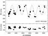 |
Fig. 1 RV curve (top panel) and rms scatter of the residual (bottom panel) for HD 66141 from December 2003 to January 2011. The solid line is the orbital solution with a period of 480.5 ± 0.5 days and an eccentricity of 0.07 ± 0.03. |
RV measurements for HD 66141 between December 2003 and January 2011.
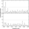 |
Fig. 2 Lomb-Scargle periodogram of the RV measurements for HD 66141. The periodogram shows a significant power at a frequency of 0.002081 ± 0.000002 c d-1 corresponding to a period of 480.5 ± 0.5 days (top panel) and after subtracting the main frequency variations (bottom panel). The horizontal dotted lines indicate an FAP threshold of 1 × 10⁻³ (0.1%). |
5. Origin of the RV variations
Evolved stars exhibit pulsations as well as surface activity, which result in low-amplitude RV variabilities on different time scales. While short-term (hours to days) RV variations have been known to be the result of stellar pulsations (Hatzes & Cochran 1998), long-term (hundreds of days) RV variations with a low-amplitude may be caused by stellar pulsations, rotational modulations by inhomogeneous surface features, or planetary companions. To establish the origin of the period for HD 66141, we examined 1) the Hipparcos and COBE/DIRBE infrared photometry; 2) the stellar chromospheric activity; 3) the spectral line bisectors; and 4) the orbital fit.
5.1. Hipparcos and COBE/DIRBE infrared photometry
We analyzed the Hipparcos photometry (ESA 1997) for HD 66141 to search for any possible brightness variations due to the rotational modulation of stellar spots. For three years, between JD 2 447 966 and JD 2 448 754, the Hipparcos satellite obtained 45 photometric measurements for HD 66141 and the data maintained a photometric stability down to the rms scatter of 0.0078 mag, corresponding to 0.17% variations. Figure 9 shows the Lomb-Scargle periodogram of these measurements. There is no significant peak near the frequency of  c d-1. Two statistically insignificant peaks are visible at frequencies
  c d-1 and
  c d-1 with FAPs of ~5 × 10⁻³, which most likely belong to 1/365.25 day = 0.00274 c d-1 artifacts. Therefore, we conclude that Hipparcos photometry does not resolve any signals of surface features such as spots.
Nearly at the same time, between JD 2 447 973 and JD 2 449 128, HD 66141 was measured in the near-infrared (NIR) 1.25, 2.2, 3.5, and 4.9μ bands by NASA’s COBE (Cosmic Backgroud Explorer) satellite with the DIRBE (Diffuse Infrared Background Experiment) instrument. The total N = 68 weekly averaged fluxes in each band were extracted for HD 66141 from the COBE/DIRBE archives (Price et al. 2010) and were used for our analysis. The Lomb-Scargle periodogram analysis of the 2.2, 3.5, and 4.9μ fluxes does not reveal any significant signals in the domain of interest, while the 1.25μ flux shows a statistically significant signal (FAP < 10-5) at the frequency of  c d-1 (
 days) with a semi-amplitude of ΔI = ± 4.0 Jy. The second statistically significant peak (FAP < 10-4) is at the lower frequency of
 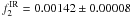 c d-1 (
 days).
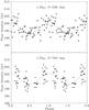 |
Fig. 3 1.25μ flux intensity measurements of HD 66141 phased to the period of the 256 (top panel) and 703 days (bottom panel). Epochs of maximum flux for 256-day and 703-day periods are JD 2 447 945.3 and JD 2 448 098.0. |
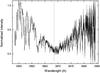 |
Fig. 4 Ca II H spectral region for HD 66141. It shows that the Ca II H core feature exhibits no emission at the line center. |
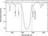 |
Fig. 5 Line profile near the Hα region for HD 66141. Two vertical dashed lines denote the range of Hα in which the EWs were measured. |
After removing the 0.00390 or 0.00142 c d-1 signals from the original data the residuals do not show any significant variations (Fig. 9). Figure 3 shows the phase curve of the original data folded with two periods  days (upper panel) and
  days (bottom panel). The 256-day and 703-day periods are within the uncertainty limits for the rotation period of 253 − 938 days found in Sect. 3.
5.2. Chromospheric activity
The EW variations of Ca II H and Hα lines are frequently used as chromospheric activity indicators. The emissions in the Ca II H core are formed in the chromosphere and show a typical central reversal in the chromospheric activity (Pasquini et al. 1988; Saar & Donahue 1997). The extra emission at the center of the line implies that the source function in the chromosphere is larger than in the photosphere. This reversal phenomenon is common in cool stars and is intimately connected to the convective envelope and magnetic activity. Unfortunately, the Ca II H line region for HD 66141 does not have a sufficient S/N to estimate EW variations (Fig. 4). However, it is strong enough to check the emission feature in the Ca II H line core, and we found no emission.
Because the Hα absorption originates in the upper layers of stellar atmosphere and is also sensitive to stellar activity (Kürster et al. 2003), we used the Hα EW to measure the variations. Owing to sparse blending lines, a weak telluric line, and a narrow Hα absorption line (Fig. 5), it is easy to estimate the Hα EW. We measured the EW using a band pass of ± 1.0 Å centered on the core of the Hα line to avoid nearby blending lines (i.e. Ti I 6561.3, Na II 6563.9, and ATM H2O 6564.0 Å). The mean EW of the Hα line in HD 66141 is measured to be 1135.7 ± 18.5 mÅ. The rms of 18.5 mÅ corresponds to a 1.6% variation in the EW. Figure 6 (top panel) shows the Hα EW variations as a function of time and the Lomb-Scargle periodogram of the Hα EW variations is shown in the middle panel of Fig. 9. There is large power at the frequency of 0.001416 ± 0.000070 c d-1 with an FAP of less than 10-5, corresponding to a period of 706.4 ± 35.0 days. Figure 7 shows the Hα EW variations phased to a period of 706 days.
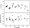 |
Fig. 6 Origin of the RV variations for HD 66141. JD vs. Hα EW variations (top panel) and the BVS variations (bottom panel) from December 2003 to January 2011. |
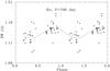 |
Fig. 7 Hα EW variations for HD 66141 phased to the period of 706 days. The same epoch of JD 2 448 098.0 found in the 1.25μ (703-day flux variations) was used. |
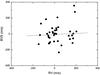 |
Fig. 8 BVS vs. RV variations for HD 66141 from December 2003 to January 2011. The dashed line marks a slope of 0.07. |
5.3. Line bisector variations
The RV variations produced by the rotational modulation of the surface inhomogeneities should produce some changes in the spectral line shape, such as line asymmetry (Queloz et al. 2001). Consequently, the variations in the shapes of spectral lines help in interpreting the origin of RV variations. The difference in the bisectors of line widths between the top and bottom of the line profile is defined as the bisector velocity span (BVS).
We measured the BVS using the least-squares deconvolution (LSD) technique (Donati et al. 1997; Reiners & Royer 2004; Glazunova et al. 2008), which is calculated by the mean profile of the spectral lines. We also used the Vienna Atomic Line Database (VALD; Piskunov et al. 1995) to prepare the list of spectral lines. A total of ~3900 lines within the wavelength region of 4500 − 4900 Å and 6450 − 6840 Å were used to construct the LSD profile, which excluded spectral regions around the I2 absorption region, hydrogen lines, and regions with strong contamination by terrestrial atmospheric lines. Then, we calculated the BVS of the mean profile between two different central depth levels, 0.8 and 0.25. BVS variations as a function of time are exhibited in Fig. 6 (bottom panel) and BVS vs. RV variations are exhibited in Fig. 8. We measured a slope of 0.07, which shows no correlation between BVS and the measured RV. The short-term accuracy of BVS measurements was measured by comparison of several spectra obtained in the same or during consecutive nights and is value of 45 m s-1. The long-term BVS scatter might indeed be larger than that of the short-term measurements. We found a scatter of 116 m s-1 for the whole BVS measurements of HD 66141. In Fig. 9 (bottom panel), the Lomb-Scargle periodogram of the BVS shows no statistically significant peaks in the domain of interest.
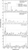 |
Fig. 9 Lomb-Scargle periodograms of the COBE/DIRBE satellite 1.25μ flux intensity measurements, the Hipparcos photometric measurements, the Hα EW variations, and the BVS variations for HD 166141 (top to bottom panel). The vertical dashed line marks the location of the period of 480 days and the horizontal dotted lines indicate an FAP threshold of 1 × 10⁻³ (0.1%). Top panel – the solid line is the Lomb-Scargle periodogram of the COBE/DIRBE satellite 1.25μ flux intensity measurements for 3.5 years. The arrows show the positions of the dominant peaks at |


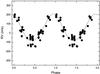 |
Fig. 10 RV measurements for HD 66141 phased to the orbital period of 480.5 days. The solid line is the orbital solution that fits the data with an rms of 38.8 m s-1. |
5.4. Orbital fit
We found that the variation was fitted best with a Keplerian orbit with a period P = 480.5 ± 0.5 days, a semi-amplitude K = 146.2 ± 2.7 m s-1, and an eccentricity e = 0.07 ± 0.03. The solid line in Fig. 1 shows the RV curve as a function of time for HD 66141 and the residuals after extracting the main frequency. The RV measurements phased to P = 480.5 days are shown in Fig. 10; they exhibit clear periodic variations at this frequency. This Keplerian orbit determines the minimum mass of a planetary companion m sin i = 6.0 ± 0.3 MJup at a distance a = 1.2 ± 0.1 AU from HD 66141. All orbital elements are listed in Table 3.
The dispersion of the RV residuals is 38.8 m s-1, which is significantly higher than the rms scatter of the RV standard star (6.7 m s-1) and the typical RV measurements error (~8 m s-1). We thus can propose that the large scatter in the residuals can be attributed to unresolved oscillations. Using the scaling relation (Eq. (7) from Kjeldsen & Bedding 1995) with a luminosity and a mass of HD 66141 (Table 2), we expect the semi-amplitude of pulsations to be 39 m s-1, which almost agrees with the 38.8 m s-1 dispersion of the residuals.
The visual inspection of the residuals also shows a long-period of about ± 50 m s-1 variations with a time-scale comparable to the time span of the observations. It is premature to discuss the origin of long-term variations until we have longer time-span observations covering several variability cycles. For completeness, we would like to mention two other exoplanet-hosting candidate K giant stars from our survey: γ1 Leo (Han et al. 2010) and α Ari (Kim et al. 2006; Lee et al. 2011). They also exhibit long-term variations of the RV residuals that are superimposed with short-term pulsational variability, which is well established from night-to-night observations.
Orbital parameters of the best-fit Keplerian orbit for HD 66141 b.
6. Discussion and conclusion
From the analysis of the eight-year precise RV measurements, we found compelling evidence for low-amplitude and long-period 480-day RV variations in the K giant HD 66141. We examined possible origins of these RV variations. The Ca II H line profile, the Hipparcos photometric measurements, and the BVS measurements show no detectable indication of variability at this period.
However, the analysis of 1.25μ COBE/DIRBE infrared flux measurements for HD 66141 revealed two periods of 256 or 703 days that fit the observed flux variations well. Judging whether a period is real was made from the EW analysis of Hα line, which revealed almost the same period of variations (703.0 ± 39.4 vs. 706.4 ± 35.0 days). Comparison of Figs. 3 and 7 clearly shows a phase lag of about 0.18 between the time of maximum Hα EW and the maximum of the 1.25μ flux. We note that the wavelength-to-wavelength phase lags are clearly present in variations of M giants and Mira variables with the optical maximum appearing about 0.18 phase before the maxima at 1.25μ (Price et al. 2010). It was shown by Alvarez & Plez (1998) that optical/NIR lags in oxygen-rich Miras are likely due to strong titanium oxide (TiO) variability during the pulsation cycle. For the K2 III star HD 66141 the TiO lines might be formed in a cool spot on the surface with a temperature contrast of about 1000 K. Thus, the temperature in the cool spot might approach about 3500 K (the typical temperature of M giants). The question about the origin of 0.18 phase lag between Hα EW and the 1.25μ flux variations needs additional confirmation and investigation.
Returning to the about 703−706-day periods of the variations in the NIR fluxes and optical absorptions in a spectral line, we note that it is very different from the RV period of 480 days. The most likely origin of the 703−706-day periods is certainly the surface spot(s) and the rotation of HD 66141. These periods are equal to each other within the accuracy, therefore we deduce a mean value Prot = 705 ± 53 days as the rotation period of the star. With the new estimate of the rotation period of HD 66141 and the accurate radius, we can accurately re-estimate the rotational velocity as vrotsini = 1.5 km s-1.
In summary, the most likely cause of the 480-day RV variations is a planet orbiting the star. HD 66141 is a planetary system with a 1.1 ± 0.1 M⊙ giant star and a 6.0 ± 0.3 MJup planet.
Acknowledgments
B.C.L. acknowledges partial support by the KASI (Korea Astronomy and Space Science Institute) grant 2012-1-410-03. Support for M.G.P. was provided by the National Research Foundation of Korea to the Center for Galaxy Evolution Research. D.E.M. acknowledges his work as part of the research activity of the National Astronomical Research Institute of Thailand (NARIT), which is supported by the Ministry of Science and Technology of Thailand. We thank the developers of the Bohyunsan Observatory Echelle Spectrograph (BOES) and all staff of the Bohyunsan Optical Astronomy Observatory (BOAO). We are grateful to the anonymous referee for useful comments that have greatly improved the quality of the manuscript. This research made use of the SIMBAD database, operated at the CDS, Strasbourg, France.
References
- Alvarez, R., & Plez, B. 1998, A&A, 330, 1109 [NASA ADS] [Google Scholar]
- Batten, A. H. 1983, Bulletin Information du Centre de Données Stellaires, 24, 3 [NASA ADS] [Google Scholar]
- Butler, R. P., Marcy, G. W., Williams, E., et al. 1996, PASP, 108, 500 [NASA ADS] [CrossRef] [Google Scholar]
- da Silva, L., Girardi, L., Pasquini, L., et al. 2006, A&A, 458, 609 [NASA ADS] [CrossRef] [EDP Sciences] [Google Scholar]
- de Medeiros, J. R., & Mayor, M. 1999, A&AS, 139, 433 [NASA ADS] [CrossRef] [EDP Sciences] [Google Scholar]
- Döllinger, M. P., Hatzes, A. P., Pasquini, L., et al. 2009, A&A, 505, 1311 [NASA ADS] [CrossRef] [EDP Sciences] [Google Scholar]
- Donati, J.-F., Semel, M., Carter, B. D., et al. 1997, MNRAS, 291, 658 [NASA ADS] [CrossRef] [MathSciNet] [Google Scholar]
- Eaton, J. A., & Williamson, M. H. 2007, PASP, 119, 886 [NASA ADS] [CrossRef] [Google Scholar]
- Endl, M., Kürster, M., & Els, S. 2000, A&A, 362, 585 [Google Scholar]
- ESA 1997, VizieR Online Data Catalog: I/239 [Google Scholar]
- Famaey, B., Jorissen, A., Luri, X., et al. 2005, A&A, 430, 165 [NASA ADS] [CrossRef] [EDP Sciences] [Google Scholar]
- Fekel, F. C. 1997, PASP, 109, 514 [NASA ADS] [CrossRef] [Google Scholar]
- Frink, S., Mitchell, D. S., Quirrenbach, A., et al. 2002, ApJ, 576, 478 [NASA ADS] [CrossRef] [MathSciNet] [Google Scholar]
- Galazutdinov, G. A. 1992, Special Astrophysical Observatory Preprint 92 (Nizhnij Arkhyz: SAO) [Google Scholar]
- Girardi, L., Bressan, A., Bertelli, G., et al. 2000, A&AS, 141, 371 [NASA ADS] [CrossRef] [EDP Sciences] [Google Scholar]
- Glazunova, L. V., Yushchenko, A. V., Tsymbal, V. V., et al. 2008, AJ, 136, 1736 [NASA ADS] [CrossRef] [Google Scholar]
- Han, I., Kim, K.-M., Lee, B.-C., et al. 2007, PKAS, 22, 75 [Google Scholar]
- Han, I., Lee, B.-C., Kim, K.-M., et al. 2008, JKAS, 41, 59 [Google Scholar]
- Han, I., Lee, B. C., Kim, K. M., et al. 2010, A&A, 509, A24 [NASA ADS] [CrossRef] [EDP Sciences] [Google Scholar]
- Hatzes, A. P., & Cochran, W. D. 1993, ApJ, 413, 339 [NASA ADS] [CrossRef] [Google Scholar]
- Hatzes, A. P., & Cochran, W. D. 1998, ASPC, 154, 311 [NASA ADS] [Google Scholar]
- Hatzes, A. P., Guenther, E. W., Endl, M., et al. 2005, A&A, 437, 743 [NASA ADS] [CrossRef] [EDP Sciences] [Google Scholar]
- Hatzes, A. P., Cochran, W. D., Endl, M., et al. 2006, A&A, 457, 335 [NASA ADS] [CrossRef] [EDP Sciences] [Google Scholar]
- Johnson, J. A., Fischer, D. A., Marcy, G. W., et al. 2007, ApJ, 665, 785 [NASA ADS] [CrossRef] [Google Scholar]
- Jørgensen, B. R., & Lindegren, L. 2005, A&A, 436, 127 [NASA ADS] [CrossRef] [EDP Sciences] [Google Scholar]
- Kharchenko, N. V., Scholz, R.-D., Piskunov, A. E., et al. 2007, Astron. Nachr., 328, 889 [NASA ADS] [CrossRef] [Google Scholar]
- Kim, K. M., Mkrtichian, D. E., Lee, B.-C., et al. 2006, A&A, 454, 839 [NASA ADS] [CrossRef] [EDP Sciences] [Google Scholar]
- Kim, K.-M., Han, I., Valyavin, G. G., et al. 2007, PASP, 119, 1052 [Google Scholar]
- Kjeldsen, H., & Bedding, T. R. 1995, A&A, 293, 87 [NASA ADS] [Google Scholar]
- Kürster, M., Hatzes, A. P., Cochran, W. D., et al. 1999, A&A, 344, L5 [NASA ADS] [Google Scholar]
- Kürster, M., Endl, M., Rouesnel, F., et al. 2003, A&A, 403, 1077 [NASA ADS] [CrossRef] [EDP Sciences] [Google Scholar]
- Lee, B.-C., Mkrtichian, D. E., Han, I., et al. 2008, AJ, 135, 2240 [NASA ADS] [CrossRef] [Google Scholar]
- Lee, B.-C., Mkrtichian, D. E., Han, I., et al. 2011, A&A, 529, A134 [NASA ADS] [CrossRef] [EDP Sciences] [Google Scholar]
- Lomb, N. R. 1976, Ap&SS, 39, 447 [NASA ADS] [CrossRef] [Google Scholar]
- Lovis, C., & Mayor, M. 2007, A&A, 472, 657 [NASA ADS] [CrossRef] [EDP Sciences] [Google Scholar]
- Massarotti, A., Latham, D. W., Stefanik, R. P., et al. 2008, AJ, 135, 209 [NASA ADS] [CrossRef] [Google Scholar]
- Niedzielski, A., Konacki, M., Wolszczan, A., et al. 2007, ApJ, 669, 1354 [NASA ADS] [CrossRef] [Google Scholar]
- Pasquini, L., Pallavicini, R., & Pakull, M. 1988, A&A, 191, 253 [NASA ADS] [Google Scholar]
- Pearce, J. A. 1955, Trans. IAU XI, 442 [Google Scholar]
- Perryman, M. A. C., Lindegren, L., Kovalevsky, J., et al. 1997, A&A, 323, L49 [NASA ADS] [Google Scholar]
- Piskunov, N. E., Kupka, F., Ryabchikova, T. A., et al. 1995, A&AS, 112, 525 [NASA ADS] [Google Scholar]
- Price, S. D., Smith, B. J., Kuchar, T. A., et al. 2010, ApJ, 190, 203 [NASA ADS] [Google Scholar]
- Queloz, D., Henry, G. W., Sivan, J. P., et al. 2001, A&A, 379, 279 [NASA ADS] [CrossRef] [EDP Sciences] [Google Scholar]
- Reffert, S., Quirrenbach, A., Mitchell, D. S., et al. 2006, ApJ, 652, 661 [NASA ADS] [CrossRef] [Google Scholar]
- Reiners, A., & Royer, F. 2004, A&A, 415, 325 [Google Scholar]
- Richichi, A., & Percheron, I. 2002, A&A, 386, 492 [NASA ADS] [CrossRef] [EDP Sciences] [Google Scholar]
- Saar, S. H., & Donahue, R. A. 1997, ApJ, 485, 319 [NASA ADS] [CrossRef] [Google Scholar]
- Sato, B., Ando, H., Kambe, E., et al. 2003, ApJ, 597, L157 [NASA ADS] [CrossRef] [Google Scholar]
- Scargle, J. D. 1982, ApJ, 263, 835 [NASA ADS] [CrossRef] [Google Scholar]
- Setiawan, J., Hatzes, A. P., von der Lühe, O., et al. 2003, A&A, 398, L19 [NASA ADS] [CrossRef] [EDP Sciences] [Google Scholar]
- Takeda, Y., Ohkubo, M., Sato, B., et al. 2005, PASJ, 57, 27 [Google Scholar]
- Tody, D. 1986, Proc. SPIE, 627, 733 [NASA ADS] [CrossRef] [Google Scholar]
- Udry, S., Mayor, M., Maurice, E., et al. 1999, ASPC, 185, 383 [Google Scholar]
- van Leeuwen, F. 2007, A&A, 474, 653 [NASA ADS] [CrossRef] [EDP Sciences] [Google Scholar]
All Tables
All Figures
|
Fig. 1 RV curve (top panel) and rms scatter of the residual (bottom panel) for HD 66141 from December 2003 to January 2011. The solid line is the orbital solution with a period of 480.5 ± 0.5 days and an eccentricity of 0.07 ± 0.03. |
| In the text | |
|
Fig. 2 Lomb-Scargle periodogram of the RV measurements for HD 66141. The periodogram shows a significant power at a frequency of 0.002081 ± 0.000002 c d-1 corresponding to a period of 480.5 ± 0.5 days (top panel) and after subtracting the main frequency variations (bottom panel). The horizontal dotted lines indicate an FAP threshold of 1 × 10⁻³ (0.1%). |
| In the text | |
|
Fig. 3 1.25μ flux intensity measurements of HD 66141 phased to the period of the 256 (top panel) and 703 days (bottom panel). Epochs of maximum flux for 256-day and 703-day periods are JD 2 447 945.3 and JD 2 448 098.0. |
| In the text | |
|
Fig. 4 Ca II H spectral region for HD 66141. It shows that the Ca II H core feature exhibits no emission at the line center. |
| In the text | |
|
Fig. 5 Line profile near the Hα region for HD 66141. Two vertical dashed lines denote the range of Hα in which the EWs were measured. |
| In the text | |
|
Fig. 6 Origin of the RV variations for HD 66141. JD vs. Hα EW variations (top panel) and the BVS variations (bottom panel) from December 2003 to January 2011. |
| In the text | |
|
Fig. 7 Hα EW variations for HD 66141 phased to the period of 706 days. The same epoch of JD 2 448 098.0 found in the 1.25μ (703-day flux variations) was used. |
| In the text | |
|
Fig. 8 BVS vs. RV variations for HD 66141 from December 2003 to January 2011. The dashed line marks a slope of 0.07. |
| In the text | |
|
Fig. 9 Lomb-Scargle periodograms of the COBE/DIRBE satellite 1.25μ flux intensity measurements, the Hipparcos photometric measurements, the Hα EW variations, and the BVS variations for HD 166141 (top to bottom panel). The vertical dashed line marks the location of the period of 480 days and the horizontal dotted lines indicate an FAP threshold of 1 × 10⁻³ (0.1%). Top panel – the solid line is the Lomb-Scargle periodogram of the COBE/DIRBE satellite 1.25μ flux intensity measurements for 3.5 years. The arrows show the positions of the dominant peaks at |
| In the text | |
|
Fig. 10 RV measurements for HD 66141 phased to the orbital period of 480.5 days. The solid line is the orbital solution that fits the data with an rms of 38.8 m s-1. |
| In the text | |
Current usage metrics show cumulative count of Article Views (full-text article views including HTML views, PDF and ePub downloads, according to the available data) and Abstracts Views on Vision4Press platform.
Data correspond to usage on the plateform after 2015. The current usage metrics is available 48-96 hours after online publication and is updated daily on week days.
Initial download of the metrics may take a while.