| Issue |
A&A
Volume 547, November 2012
|
|
|---|---|---|
| Article Number | A20 | |
| Number of page(s) | 7 | |
| Section | Stellar structure and evolution | |
| DOI | https://doi.org/10.1051/0004-6361/201219717 | |
| Published online | 22 October 2012 | |
Neutron star masses from hydrodynamical effects in obscured supergiant high mass X-ray binaries
1
ISDC Data Center for Astrophysics, Université de Genève,
Chemin d’Ecogia 16,
1290
Versoix,
Switzerland
e-mail: This email address is being protected from spambots. You need JavaScript enabled to view it.
2
Observatoire de Genève, Université de Genève,
Chemin des Maillettes 51,
1290
Versoix,
Switzerland
3
Department of Physics, North Carolina State
University, Raleigh,
NC
27695-8202,
USA
Received: 30 May 2012
Accepted: 5 September 2012
Abstract
Context. A population of obscured supergiant high mass X-ray binaries has been discovered by INTEGRAL. X-ray wind tomography of IGR J17252-3616 inferred a slow wind velocity to account for the enhanced obscuration.
Aims. The main goal of this study is to understand under which conditions high obscuration could occur.
Methods. We have used an hydrodynamical code to simulate the flow of the stellar wind around the neutron star. A grid of simulations was used to study the dependency of the absorbing column density and of the X-ray light-curves on the model parameters. A comparison between the simulation results and the observations of IGR J17252-3616 provides an estimate on these parameters.
Results. We have constrained the wind terminal velocity to 500−600 km s-1 and the neutron star mass to 1.75−2.15 M⊙.
Conclusions. We have confirmed that the initial hypothesis of a slow wind velocity with a moderate mass loss rate is valid. The mass of the neutron star can be constrained by studying its impact on the accretion flow.
Key words: X-rays: binaries / methods: numerical / stars: winds, outflows / stars: neutron / accretion, accretion disks
New address: Nicolaus Copernicus Astronomical Center, Polish Academy of Sciences, Bartycka 18, 00-716 Warszawa, Poland e-mail: This email address is being protected from spambots. You need JavaScript enabled to view it.
© ESO, 2012
1. Introduction
In classical supergiant high mass X-ray binaries (sgHMXBs) neutron stars are orbiting at a distance of α ~ 1.5−2 R∗ from their companion stars. The donors, in these systems, are OB supergiants with mass loss rates on the order of ~10-6 M⊙ yr-1 and wind terminal velocities of ~1500 km s-1.
Blondin et al. (1990, 1991) modeled the interactions between the neutron star and the stellar wind in Vela X-1 and revealed that the wind of the massive star is disrupted by the gravity and photoionization of the neutron star. The imprint of these two parameters can be observed in the variability of the absorbing column density with orbital phase. High-resolution soft X-ray spectroscopy of the brightest sources revealed a number of lines in emission, constraining the ionization level of the gas (Watanabe et al. 2006).
The heavily obscured sgHMXBs (Walter et al. 2006) share some of the characteristics of the classical sgHMXBs. The main difference between classical and obscured sgHMXBs is that the latter ones are much more absorbed in the X-rays. The absorbing column density (NH ≳ 1023 cm-2) is, on average, 10 times larger than in classical systems and well above the galactic absorption in the direction of the sources.
The obscured sgHMXB IGR J17252−3616 (=EXO 1722-363; Walter et al. 2006; Zurita Heras et al. 2006; Thompson et al. 2007) is an eclipsing binary hosting a pulsar with Ps ~ 414 s, an orbital period of Po ~ 9.74 days, and an orbital radius of α ≈ 1.75 R∗. Ground-based observations (Mason et al. 2009, 2010) showed that the donor star is likely a B0-5I or B0-1 Ia. Optical and infrared (IR) observations confirmed the supergiant nature and showed prominent P-Cygni profile (Chaty et al. 2008).
To explain the XMM-Newton and INTEGRAL observations, Manousakis & Walter (2011, hereafter MW11) suggested that the wind terminal velocity of the system is relatively, low, on the order of υ∞ ~ 500 km s-1. An ad hoc modeling of a hydrodynamic trailing tail allowed to reproduce the observed column density profile and the observed iron Fe Kα line emissivity.
In the present paper, we have used the hydrodynamic code VH-1 to study the wind dynamics of IGR J17252-3616 under the assumption of a slow wind velocity. We start with a description of the hydrodynamic code and of the grid of simulations in Sect. 2, the results are presented in Sect. 3 and discussed in Sect. 4, followed by the conclusions in Sect. 5.
2. Hydrodynamical simulations
2.1. The hydrodynamical code
The full description of the VH-11 hydrodynamical code is given in Blondin et al. (1990, 1991). To simulate sgHMXB the code accounts for: i) the gravity of the primary and of the neutron star; ii) the radiative acceleration of the stellar wind of the primary star; and iii) the suppression of the stellar wind acceleration in the Strömgren sphere of the neutron star. The simulations take place in the orbital plane, reducing the problem to two dimensions. The code uses the piecewise parabolic method developed by Colella & Woodward (1984).
A computational grid of 600 radial by 247 angular zones, extending from 1 to ~15 R∗ and in angle from −π to + π, has been employed. The grid structure is nonuniform, with cells size decreasing towards the neutron star. The maximal resolution, reached close to the neutron star, is δR ~ 1010 cm ~ racc/3, where  is the accretion radius (Bondi & Hoyle 1944).
The neutron star in IGR J17252-3616 orbits in a almost circular (e < 0.15) and highly inclined (i > 80°) orbit (Manousakis & Walter 2011). Therefore, a circular (e = 0) and edge-on (i = 90°) orbit is assumed for simplicity. As most of the absorption comes from the accretion stream, close to the neutron star (within 1012 cm), the variability of the absorbing column density with orbital phase does not depend on small variations of the inclination angle.
The code produces density and ionization ( , where LX is the average X-ray luminosity, n is the number density at the distance rns from the neutron star; Tarter et al. 1969) maps that are stored. These allow to determine the simulated column density. As short time-scale variations occurs, we have calculated the time-averaged orbital phase resolved column density and its 3σ variability. The 3D instantaneous mass accretion rate (Ṁacc) onto the neutron star is also recorded by translating the 2D instantaneous mass accretion rate along the rim of the accretion radius, racc. From the mass accretion rate, we can infer the instantaneous X-ray luminosity of the neutron star. For each simulations, the code was run for about 6 to 8 orbits, corresponding to about 60−80 days. This is enough for the wind to reach a stable configuration. The relaxation time is on the order of 0.8 orbits. The first 10 days of the simulations are therefore excluded from our analysis.
Although 3D hydrodynamic simulations are poorly studied in HMXB, differences between 2D and 3D are expected. In general, 3D simulations increase the instabilities and fluctuations. These effects have been studied in the idealized case of Hoyle-Lyttleton accretion (Taam & Fryxell 1988; Ruffert 1999; Blondin & Raymer 2012) and in accreting pulsars where a formation of a planar accretion disk is expected from 2D codes, whilst accretion in 3D is unstable, allowing the formation of filamentary structures (Ruffert & Arnett 1994).
2.2. Stellar wind acceleration
The winds of hot massive stars are characterized, observationally, by the wind terminal velocity and mass-loss rate. The velocity is described by the β-velocity law, υ = υ∞(1 − R∗/r) β where υ∞ is the terminal velocity and β is the gradient of the velocity field. For supergiant stars, values for wind terminal velocities and mass-loss rates are in the range υ∞ ~ 500−3000 km s-1 and Ṁw ~ 10-7−10-5 M⊙ yr-1, respectively (Kudritzki & Puls 2000). The donor star typically weights M∗ ≳ 10 M⊙ with a radius of R∗ ≳ 1012 cm.
The winds of massive supergiant stars are radiatively driven by absorbing photons from the photosphere (Castor et al. 1975, hereafter CAK). The modeling of stellar wind is complicated by the fact that the radiation force is known to be unstable (Owocki & Rybicki 1984). We use the CAK/Sobolev approximations with the finite disk correction (Friend & Abbott 1986) which produces a smooth stellar wind with β = 0.8. However, regions in the stellar wind can differ from the predictions of the CAK/Sobolev approximation when growth of instabilities are taken into account (Owocki et al. 1988).
2.3. Photoionization
The radiative acceleration of the wind from the donor star primarily occurs due to the UV line transitions that are suppressed by X-ray ionization. The effects of X-ray ionization on the radiative acceleration force are complicated due to the large number of ions and line transitions which contribute to the UV opacity (Stevens & Kallman 1990). A critical ionization parameter can be defined, above which the radiative force is negligible. For ξ > 102.5 erg cm s-1, most of the elements responsible for the wind acceleration are fully ionized and, therefore, the radiatively acceleration force vanishes. At that level, light atoms (e.g. H) are fully ionized and do not contribute to the absorbing column density while heavier atoms (e.g. C, N, O) are highly ionized (Kallman & McCray 1982).
The main effect of the ionization is the enhancement of the mass accretion rate onto the compact object. The acceleration cutoff also triggers the formation of a dense wake at the rim of the Strömgren zone (Fransson & Fabian 1980), and has an impact on the absorption at late orbital phases. X-ray ionization can also affect the thermal state of the wind through X-ray heating and radiative cooling, which can create additional filamentary structures in the wind, with slightly different time-averaged absorbing column density (Blondin et al. 1990).
2.4. Parametrization
In order to simulate IGR J17252-3616, we proceed in two steps. We started by investigating the parametrization of the stellar wind of the donor star. This is achieved using a 1D simulation assuming spherical symmetry. Spectral classification allowed to constrain the donor star parameters (Chaty et al. 2008; Mason et al. 2009, 2010). In our analysis we have adopted an effective temperature of Teff = 30 000 K, a stellar luminosity of L∗ = 4 × 10⁵ L⊙, and a stellar radius of R∗ = 29 R⊙. The mass of the donor star is assumed to be M∗ = 15 M⊙ (Takeuchi et al. 1990; Thompson et al. 2007).
Parameters of the 2D simulations.
The wind acceleration depends on the CAK-k and CAK-α parameters representing the number and strength of the absorption lines, and ρ0, the density at the surface of the donor star. Each of the triplet (k, α, ρ0) produces a monotonically increasing wind velocity. Validation of the wind is performed by fitting the β-velocity law to the simulated data which returns the wind terminal velocity and the gradient of the velocity field. The β parameter was found to be ~0.8 in all cases and the terminal velocity ranged between 500 and 1200 km s-1. The corresponding mass-loss rate (using the continuity equation) is ranging from 2 × 10⁻⁷ M⊙ yr-1 to 5 × 10⁻⁶ M⊙ yr-1. Table 1 shows the CAK parameters and the corresponding mass-loss rates and terminal velocities. Although the stellar parameters are fixed in our simulations, observational uncertainties are present. The simulated absorbing column density profile can be affected by these uncertainties (see Sect. 4.2 for more details).
We used the above CAK parameters to trigger the 2D simulations. The system now hosts a neutron star of mass MX (in M⊙), having a luminosity LX = 1036 erg s-1 (MW11), placed at a distance α (in R∗) from its donor. A grid of parameters with varying α and MX was used to simulate the system. The parameters are listed in Table 1.
3. Results
3.1. Wind terminal velocity and mass-loss rate
In order to study and constrain the dependency of the absorbing column density on the wind properties, we built a grid of simulation for a variety of mass-loss rates and wind terminal velocities. We have used two wind terminal velocities (500 km s-1 and 1200 km s-1). and mass-loss rates of (0.2,1,5) × 10-6 M⊙ yr-1. The orbital radius is fixed to α = 1.75 R∗ and the mass of the neutron star varies in the range 1.55, 1.75, and 1.95 M⊙. Six wind configurations (CAK-α, CAK-k, ρ0) were simulated for each of these masses. These parameters are listed in Table 1 (group 1).
The geometry of the shock, formed around the neutron star, is affected by the wind parameters and by the ionization. The position and orientation of the bow shock depends on the relative velocity of the neutron star within the wind and on the X-ray luminosity.
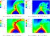 |
Fig. 1 Density distribution (g cm-3; color bar) in the plane of the orbit after ~3 orbits for a neutron star mass of MX = 1.95 M⊙ and different wind parameters. (This figure is available in color in electronic form.) |
Figure 1 shows the density maps (after 3 orbits) for some wind configurations. The orientation of the bow shock and accretion wake (tail) depends on the mass-loss rate and wind terminal velocity. For the slow wind, the accretion wake is always visible, enhanced, and tilted. For a wind velocity of 1200 km s-1, the accretion wake is not that tilted. For a mass loss rate of Ṁ = 2 × 10⁻⁷ M⊙ yr-1, the accretion wake is much weakened.
Figure 2 shows the time-averaged simulated absorbing column density as a function of orbital phase, for MX = 1.95 M⊙ with the observations of IGR J17252−3616. All these profiles show some common characteristics. At early phases, the smooth wind component dominates, followed by a rise of NH (orbital phase ~0.3), representing the bow shock and the accretion wake. Then, the absorption roughly remains at a constant level. The tidal stream between the donor and neutron star also influences the absorbing column density at later phases.
Among these curves, only one simulation can represent the data (v5.0_ML10_A175_MN195) suggesting a wind terminal velocity of υ∞ = 500 km s-1 and a mass loss rate of Ṁ = 10-6 M⊙ yr-1. The dependency of the absorbing column density orbital profile with the mass of the neutron star and binary separation parameters are discussed in Sects. 3.2 and 3.3, respectively.
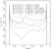 |
Fig. 2 Time-averaged simulated absorbing column density (NH) (group 1 in Table 1). The mass of the neutron star is fixed to MX = 1.95 M⊙. The data points are from MW11. |
3.2. Mass of the neutron star
A group of simulations was implemented with neutron star masses varying between 1.5 and 2.0 M⊙. The summary of these simulations is given in Table 1 (group 2). The separation and the wind parameters are identical to those of the model v5.0_ML10_A175_MN195.
Figure 4 shows the density maps (after ~3 orbits). The corresponding time-averaged absorbing column density is plotted in Fig. 3. The heavier the neutron star, the more bended the accretion wake. This effect is revealed in the orbital phase dependency of the absorbing column density, moving the position of the minimum to earlier phases. For an heavier neutron star, more gas will accumulate and the absorption will get stronger. We can therefore estimate, in the frame of our model, that the mass of the neutron star is in the range MNS = 1.9−2.0 M⊙ (see Fig. 3).
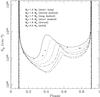 |
Fig. 3 Time-averaged simulated absorbing column density (NH) for various neutron star masses (group 2 in Table 1). The stellar wind is characterised by a Ṁ = 1 × 10⁻⁶ M⊙ yr-1 and υ∞ = 500 km s-1. The data points are from MW11. |
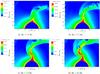 |
Fig. 4 Density distribution (g cm-3; color bar) in the plane of the orbit after ~3 orbits with a terminal velocity of υ∞ ≈ 500 km s-1 and a mass-loss rate Ṁw ≈ 10-6 M⊙ yr-1. The mass of the neutron star scales from 1.5 to 2.0 M⊙. See the text for more details. (This figure is available in color in electronic form.) |
3.3. Binary separation
The wind structure is also affected by the binary separation. When the neutron star is closer to the donor star, the tidal stream between the two stars is enhanced. This effect is maximized when the donor star fills its Roche lobe. In classical and obscured sgHMBs it is very likely that the evolved companion is close to filling its Roche lobe. Therefore, tidal connection between the two stars enhances the absorbing column density (Blondin et al. 1991).
Figure 5 shows the absorbing column density for various wind terminal velocities. In these plots there is an indication that for a combination of neutron star mass and binary separation we sustain a roughly constant obscuration. Table 2 gives the χ2 of the simulation (from Fig. 5) accounting for both the error bars of the data and temporal variations of the absorbing column density. The data can be represented by the model with a wind terminal velocity, neutron star mass, and binary separation in the range of 500−600 km s-1, 1.85−1.95 M⊙, and 1.74−1.75 R∗, respectively.
The χ2 for models for various neutron star masses, binary separations, and wind terminal velocities.
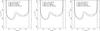 |
Fig. 5 Time-averaged absorbing column density (NH) for various parameters (see group 3 in Table 1). The stellar wind is characterized by Ṁ = 1 × 10⁻⁶ M⊙ yr-1. The data points are from MW11. |
3.4. Statistical analysis of the X-ray light-curve
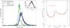 |
Fig. 6 Results from the simulation v5.5_ML10_A175_MN195. Left: the histogram of observed light-curve (black), the background fluctuation (green), and the convolution of the simulated data with the latter (blue). The inset shows the corresponding distribution of the simulated. light-curve (black) with a log-normal fit (red dashed curve). Right: the corresponding simulated time-averaged absorbing column density, together with its 99 % temporal variability, and the observed data from MW11. (This figure is available in color in electronic form.) |
We have compared the observed X-ray light-curves of IGR J17252−3616 with these derived from our simulations. The observed light-curves of IGR J17252−3616 were obtained form the INTEGRAL (Winkler et al. 2003) soft γ-ray imager ISGRI (Lebrun et al. 2003) in the energy range 20−60 keV using the HEAVENS2 interface (Walter et al. 2010).
Light-curves were built using data from the source and from a source free near-by region, using 1-h, 3-h, 6-h and 12-h time-bins and flux histograms were constructed. To achieve a relatively narrow width for the background fluctuations and a good time resolution, we selected the 6-h time-bins for our analysis.
The histogram of the observed fluxes can be fitted with normal (Gaussian) distributions. The observations can be characterized by a mean count rate of μ = 1.1 cps and a width σ = 1.0 cps for the source and μ = 0 cps with a width σ = 0.6 cps for the background (black and green lines in Fig. 6).
We performed a statistical analysis of the simulated light-curves which have been built using the mass accretion rates derived from the hydrodynamical simulations, translated into the instantaneous luminosity using  , where η = 0.1. One should notice that the input parameter LX = 1036 erg s-1 = const. (see Sect. 2) and the instantaneous X-ray luminosity are not the same. However, the average Lacc is within the 10% of the input parameter LX. The Lacc histogram can be fitted by a log-normal distribution (see inset of Fig. 6). The lognormal fit resulted in a luminosity LX ~ 1.1 × 1036 erg s-1 having a width of σ = 0.44 for model v5.5_ML10_A175_MN195.
To compare the simulated distributions with the observed ones, we convolved the simulated data with the background fluctuations (blue curves in Fig. 6). We, also, plotted the simulated NH for this model together with its 99% temporal variability (right panel of Fig. 6).
4. Discussion
4.1. Wind terminal velocities in obscured systems
The wind terminal velocities of supergiant OB stars is correlated with the effective temperature (for a review see Kudritzki & Puls 2000). For supergiant stars wind terminal velocities scales from 300 km s-1 (for Teff = 10 kK) to 3000 km s-1 (for Teff = 40 kK). An imprint of these outflows is observed in the P-Cygni profiles of UV/Optical lines. For the system IGR J17252-3616, Optical/IR studies are difficult due to high interstellar absorption (Rahoui et al. 2008).
For IGR J17252-3616, we suggested a wind terminal velocity of 500−600 km s-1 which is about 2−3 times less than expected for an OB supergiant of the same spectral type and effective temperature. The wind in massive binaries can be slower than in isolated OB stars. The neutron star can indeed cut-off the acceleration by ionizing the local environment (Stevens & Kallman 1990). Note that the peculiar X-ray binary, GX 301-2, hosting a massive early type star (Wray 977), also features a low wind terminal velocity of υ∞ ~ 500 km s-1 (Kaper et al. 2006). The column density in this system reaches ~1024 cm-2 and is interpreted as the signature of a high density stream (Leahy & Kostka 2008). In this context, it is also interesting to remark that some intermediately obscured sgHMXBs, such as 4U 1907 + 09, feature intermediate wind terminal velocity in the range ~1000 km s-1 (Kostka & Leahy 2010).
4.2. The mass of the neutron star
The neutron star mass determined by the hydrodynamical simulations is independent from the mass function derived from dynamical studies. However, it is model-dependent and uncertainties on the modelization of the wind may have an impact. Figures 3 and 5 show that the mass of the neutron star is in the range MX = 1.85−1.95 M⊙. This mass is below the theoretical maximum mass of a neutron star,  (Müller & Serot 1996).
The mass of the neutron star and the orbital radius are degenerate as seen in Fig. 5. However, this degeneracy cannot allow very large or small masses of the neutron star (see Table 2). The eclipse duration constrains the binary separation from 1.7 to 1.8 R∗ (MW11) and therefore the mass can scale from 1.85 to 2.0 M⊙. A rather heavy neutron star is needed in any case to account for the observed profile.
Radial velocity studies of the source, using VLT, provided estimates on the masses of the neutron star and donor star in the range MNS = 1.46 ± 0.38 M⊙ and MOB = 13.6 ± 1.6 M⊙ for Roche lobe overflow; MNS = 1.63 ± 0.38 M⊙ and MOB = 15.2 ± 1.6 M⊙ for an edge-on view (Mason et al. 2010). In both cases the mass of the neutron star is consistent with our results.
The companion radius and mass are obtained from the duration of the eclipse and stellar classification from mid-IR spectroscopy. These values are subject to observational uncertainties. To study the effects of these uncertainties on the determination of the mass of neutron star, we ran simulations of our best model for M∗ = 15 ± 1 M⊙ and R∗ = 29 ± 3 R⊙. The effect of the stellar radius on MNS scales as MNS(R∗) ∝ 0.069 R∗. Given the range of acceptable stellar radius (i.e., 26 to 32), the resulting neutron star’s mass range varies from 1.75 M⊙ to 2.15 M⊙. The impact of the donor’s mass on MNS scales as MNS(M∗) ∝ 0.13 M∗, resulting in, MNS = 1.8−2.1 M⊙.
Other supergiant HMXBs also feature large neutron star masses. Vela X-1 hosts a neutron star with mass in the range MX = 1.88 ± 0.13 M⊙ (Quaintrell et al. 2003) and 4U 1700-302 in the range MX = 2.44 ± 0.27 M⊙ (Clark et al. 2002). Although the sample is small, masses of neutron star in sgHMXBs, favors normal nucleonic EOSs (Lattimer & Prakash 2007).
5. Conclusions
In this paper we compare the observed properties with the results of hydrodynamic simulations of the heavily obscured sgHMXB IGR J17252-3616. Our conclusions are:
-
A low wind terminal velocity, υ∞ = 500−600 km s-1, is needed to explain the observations. A higher wind terminal velocity cannot produce enough obscuration to account for the observations.
-
The neutron star mass can be constrained from the variability of the absorbing column density along the orbital phase. In the case of IGR J17252-3616 the mass of the neutron star is in the range 1.75−2.15 M⊙.
-
The separation of the system can be limited in the range α = 1.73−1.75 R∗.
Measuring the variability of the absorbing column density with the orbital phase in obscured sgHMXBs provides an independent constraint on the mass of neutron stars.
References
- Blondin, J. M., & Raymer, E. 2012, ApJ, 752, 30 [NASA ADS] [CrossRef] [Google Scholar]
- Blondin, J. M., Kallman, T. R., Fryxell, B. A., & Taam, R. E. 1990, ApJ, 356, 591 [NASA ADS] [CrossRef] [Google Scholar]
- Blondin, J. M., Stevens, I. R., & Kallman, T. R. 1991, ApJ, 371, 684 [NASA ADS] [CrossRef] [Google Scholar]
- Bondi, H., & Hoyle, F. 1944, MNRAS, 104, 273 [NASA ADS] [CrossRef] [Google Scholar]
- Castor, J. I., Abbott, D. C., & Klein, R. I. 1975, ApJ, 195, 157 [NASA ADS] [CrossRef] [Google Scholar]
- Chaty, S., Rahoui, F., Foellmi, C., et al. 2008, A&A, 484, 783 [NASA ADS] [CrossRef] [EDP Sciences] [Google Scholar]
- Clark, J. S., Goodwin, S. P., Crowther, P. A., et al. 2002, A&A, 392, 909 [NASA ADS] [CrossRef] [EDP Sciences] [Google Scholar]
- Colella, P., & Woodward, P. R. 1984, J. Comp. Phys., 54, 174 [Google Scholar]
- Fransson, C., & Fabian, A. C. 1980, A&A, 87, 102 [NASA ADS] [Google Scholar]
- Friend, D. B., & Abbott, D. C. 1986, ApJ, 311, 701 [NASA ADS] [CrossRef] [Google Scholar]
- Kallman, T. R., & McCray, R. 1982, ApJS, 50, 263 [NASA ADS] [CrossRef] [Google Scholar]
- Kaper, L., van der Meer, A., & Najarro, F. 2006, A&A, 457, 595 [NASA ADS] [CrossRef] [EDP Sciences] [Google Scholar]
- Kostka, M., & Leahy, D. A. 2010, MNRAS, 407, 1182 [NASA ADS] [CrossRef] [Google Scholar]
- Kudritzki, R., & Puls, J. 2000, ARA&A, 38, 613 [NASA ADS] [CrossRef] [Google Scholar]
- Lattimer, J. M., & Prakash, M. 2007, Phys. Rep., 442, 109 [NASA ADS] [CrossRef] [Google Scholar]
- Leahy, D. A., & Kostka, M. 2008, MNRAS, 384, 747 [NASA ADS] [CrossRef] [Google Scholar]
- Lebrun, F., Leray, J. P., Lavocat, P., et al. 2003, A&A, 411, L141 [NASA ADS] [CrossRef] [EDP Sciences] [Google Scholar]
- Manousakis, A., & Walter, R. 2011, A&A, 526, A62 (MW11) [NASA ADS] [CrossRef] [EDP Sciences] [Google Scholar]
- Mason, A. B., Clark, J. S., Norton, A. J., Negueruela, I., & Roche, P. 2009, A&A, 505, 281 [NASA ADS] [CrossRef] [EDP Sciences] [Google Scholar]
- Mason, A. B., Norton, A. J., Clark, J. S., Negueruela, I., & Roche, P. 2010, A&A, 509, A79 [NASA ADS] [CrossRef] [EDP Sciences] [Google Scholar]
- Müller, H., & Serot, B. D. 1996, Nucl. Phys. A, 606, 508 [NASA ADS] [CrossRef] [Google Scholar]
- Owocki, S. P., & Rybicki, G. B. 1984, ApJ, 284, 337 [NASA ADS] [CrossRef] [Google Scholar]
- Owocki, S. P., Castor, J. I., & Rybicki, G. B. 1988, ApJ, 335, 914 [NASA ADS] [CrossRef] [Google Scholar]
- Quaintrell, H., Norton, A. J., Ash, T. D. C., et al. 2003, A&A, 401, 313 [NASA ADS] [CrossRef] [EDP Sciences] [Google Scholar]
- Rahoui, F., Chaty, S., Lagage, P., & Pantin, E. 2008, A&A, 484, 801 [NASA ADS] [CrossRef] [EDP Sciences] [Google Scholar]
- Ruffert, M. 1999, A&A, 346, 861 [NASA ADS] [Google Scholar]
- Ruffert, M., & Arnett, D. 1994, ApJ, 427, 351 [NASA ADS] [CrossRef] [Google Scholar]
- Stevens, I. R., & Kallman, T. R. 1990, ApJ, 365, 321 [NASA ADS] [CrossRef] [Google Scholar]
- Taam, R. E., & Fryxell, B. A. 1988, ApJ, 327, L73 [NASA ADS] [CrossRef] [Google Scholar]
- Takeuchi, Y., Koyama, K., & Warwick, R. S. 1990, PASJ, 42, 287 [NASA ADS] [Google Scholar]
- Tarter, C. B., Tucker, W. H., & Salpeter, E. E. 1969, ApJ, 156, 943 [NASA ADS] [CrossRef] [Google Scholar]
- Thompson, T. W. J., Tomsick, J. A., in ’tZand, J. J. M., Rothschild, R. E., & Walter, R. 2007, ApJ, 661, 447 [NASA ADS] [CrossRef] [Google Scholar]
- Walter, R., Zurita Heras, J., Bassani, L., et al. 2006, A&A, 453, 133 [NASA ADS] [CrossRef] [EDP Sciences] [Google Scholar]
- Walter, R., Rohlfs, R., Meharga, M. T., et al. 2010, in Proc. 8th INTEGRAL Workshop The Restless Gamma-ray Universe (INTEGRAL 2010), 162 [Google Scholar]
- Watanabe, S., Sako, M., Ishida, M., et al. 2006, ApJ, 651, 421 [NASA ADS] [CrossRef] [Google Scholar]
- Winkler, C., Courvoisier, T., Di Cocco, G., et al. 2003, A&A, 411, L1 [NASA ADS] [CrossRef] [EDP Sciences] [Google Scholar]
- Zurita Heras, J. A., de Cesare, G., Walter, R., et al. 2006, A&A, 448, 261 [NASA ADS] [CrossRef] [EDP Sciences] [Google Scholar]
All Tables
The χ2 for models for various neutron star masses, binary separations, and wind terminal velocities.
All Figures
|
Fig. 1 Density distribution (g cm-3; color bar) in the plane of the orbit after ~3 orbits for a neutron star mass of MX = 1.95 M⊙ and different wind parameters. (This figure is available in color in electronic form.) |
| In the text | |
|
Fig. 2 Time-averaged simulated absorbing column density (NH) (group 1 in Table 1). The mass of the neutron star is fixed to MX = 1.95 M⊙. The data points are from MW11. |
| In the text | |
|
Fig. 3 Time-averaged simulated absorbing column density (NH) for various neutron star masses (group 2 in Table 1). The stellar wind is characterised by a Ṁ = 1 × 10⁻⁶ M⊙ yr-1 and υ∞ = 500 km s-1. The data points are from MW11. |
| In the text | |
|
Fig. 4 Density distribution (g cm-3; color bar) in the plane of the orbit after ~3 orbits with a terminal velocity of υ∞ ≈ 500 km s-1 and a mass-loss rate Ṁw ≈ 10-6 M⊙ yr-1. The mass of the neutron star scales from 1.5 to 2.0 M⊙. See the text for more details. (This figure is available in color in electronic form.) |
| In the text | |
|
Fig. 5 Time-averaged absorbing column density (NH) for various parameters (see group 3 in Table 1). The stellar wind is characterized by Ṁ = 1 × 10⁻⁶ M⊙ yr-1. The data points are from MW11. |
| In the text | |
|
Fig. 6 Results from the simulation v5.5_ML10_A175_MN195. Left: the histogram of observed light-curve (black), the background fluctuation (green), and the convolution of the simulated data with the latter (blue). The inset shows the corresponding distribution of the simulated. light-curve (black) with a log-normal fit (red dashed curve). Right: the corresponding simulated time-averaged absorbing column density, together with its 99 % temporal variability, and the observed data from MW11. (This figure is available in color in electronic form.) |
| In the text | |
Current usage metrics show cumulative count of Article Views (full-text article views including HTML views, PDF and ePub downloads, according to the available data) and Abstracts Views on Vision4Press platform.
Data correspond to usage on the plateform after 2015. The current usage metrics is available 48-96 hours after online publication and is updated daily on week days.
Initial download of the metrics may take a while.