| Issue |
A&A
Volume 547, November 2012
|
|
|---|---|---|
| Article Number | A89 | |
| Number of page(s) | 12 | |
| Section | The Sun | |
| DOI | https://doi.org/10.1051/0004-6361/201118238 | |
| Published online | 01 November 2012 | |
Inferring the magnetic field vector in the quiet Sun
II. Interpreting results from the inversion of Stokes profiles
1
Kiepenheuer-Institut für Sonnenphysik,
Schöneckstr. 6,
79110
Freiburg,
Germany
e-mail: This email address is being protected from spambots. You need JavaScript enabled to view it.
2
Max-Planck Institut für Sonnensystemforschung,
Max-Planck Str. 2,
37191
Katlenburg-Lindau,
Germany
e-mail: This email address is being protected from spambots. You need JavaScript enabled to view it.
Received:
11
October
2011
Accepted:
1
August
2012
Abstract
In a previous paper, we argued that the inversion of Stokes profiles applied to spectropolarimetric observations of the solar internetwork yield unrealistically large values of the inclination of the magnetic field vector (γ). This is because photon noise in Stokes Q and U are interpreted by the inversion code as valid signals, that leads to an overestimation of the transverse component B⊥, thus the inclination γ. However, our study was based on the analysis of linear polarization signals that featured only uncorrelated noise. In this paper, we develop this idea further and study this effect in Stokes Q and U profiles that also show correlated noise. In addition, we extend our study to the three components of the magnetic field vector, as well as the magnetic filling factor α. With this, we confirm the tendency to overestimate γ when inverting linear polarization profiles that, although non-zero, are still below the noise level. We also establish that the overestimation occurs mainly for magnetic fields that are nearly vertical γ ≲ 20°. This indicates that a reliable inference of the inclination of the magnetic field vector cannot be achieved by analyzing only Stokes I and V. In addition, when inverting Stokes Q and U profiles below the noise, the inversion code retrieves a randomly uniform distribution of the azimuth of the magnetic field vector φ. To avoid these problems, we propose only inverting Stokes profiles for which the linear polarization signals are sufficiently above the noise level. However, this approach is also biased because, in spite of allowing for a very accurate retrieval of the magnetic field vector from the selected Stokes profiles, it selects only profiles arising from highly inclined magnetic fields.
Key words: Sun: surface magnetism / magnetic fields / Sun: photosphere / stars: magnetic field
© ESO, 2012
1. Introduction
Spectropolarimetry, which is the study of the polarization properties of the light observed in spectral lines, is the most developed and widely used tool for retrieving the magnetic properties of the solar plasma and other astrophysical objects (Stenflo 2002; Mathys 2002, and references therein). The inference of the magnetic field vector from spectropolarimetric observations is performed through the inversion of the radiative transfer equation for polarized light (del Toro Iniesta 2003a; Bellot Rubio 2004; Ruiz Cobo 2007). However, as the module of the magnetic field vector decreases, the observed signals disappear below the level of the photon noise, making the inference of the magnetic field very difficult and plagued with problems and uncertainties. This is, for instance, the case for the areas on the solar surface referred to as the solar internetwork. Here, the polarization signals are so weak that for a long time the internetwork was thought to be void of magnetic fields. With the advancements in the sensitivity of the polarimeters and the higher spatial resolution of the observations achievable with adaptive-optic systems and large-aperture telescopes, polarization signals are now routinely detected everywhere in the internetwork (Lites et al. 1996). This demonstrates that these regions are truly pervaded by magnetic fields. Unfortunately, the signals are barely above the noise level, thus it has not yet been possible to fully characterize the magnetic field vector in these regions. This has led to a long-standing controversy about the distribution of the module of the magnetic field vector in the internetwork (Domínguez Cerdeña et al. 2003; Socas-Navarro & Lites 2004; Sánchez Almeida 2005; Martínez González et al. 2006; Asensio Ramos et al. 2007; López Ariste et al. 2007; Socas-Navarro et al. 2008; see also references therein).
More recently, further discrepancies have emerged about the angular distribution of the magnetic field vector (Lites et al. 2007, 2008; Orozco Suárez et al. 2007a,b; Martínez González et al. 2008; Asensio Ramos 2009; Stenflo 2010; Ishikawa & Tsuneta 2011; Borrero & Kobel 2011). In Borrero & Kobel (2011; hereafter referred to as Paper I), we argued that the photon noise leads to a systematic overestimation of the inclination of the magnetic field vector. We reached this conclusion because when employing only vertical magnetic fields to synthesize Stokes profiles, these could be retrieved as highly inclined ones due to the sole effect of the photon noise. Since those tests were carried out with vertical magnetic fields, the linear polarization signals (Stokes Q and U) were zero. This limits the validity of the tests, as the inversion code analyzes only linear polarization profiles featuring uncorrelated noise. It is therefore worth considering the case where small linear-polarization signals (due to non-vertical magnetic fields) can be hidden below the noise. This introduces correlations that could be employed by the inversion algorithms to retrieve useful information about the inclination of the magnetic field vector. This paper is devoted to addressing this particular situation. To this end, we employ uniform distributions of the magnetic field vector (Sect. 2) to produce a large database of Stokes profiles. Therefore, unlike Paper I, the resulting Stokes profiles will have non-zero linear polarization profiles. After adding noise to these profiles, we apply an inversion algorithm (Sect. 3) that attempts to retrieve the original distribution of the magnetic field vector. Our results are described in Sects. 4 and 5. Section 6 summarizes our findings.
2. Synthesis with uniform distributions
To study the effect of the photon noise and selection criterion, we performed several
numerical experiments employing a probability distribution function that is parametrized by
the physical parameters of a Milne-Eddington atmosphere (ME). These physical parameters are
denoted as X![Mathematical equation: \begin{equation} \ve{X} = [\ve{B}, \alpha, V_{\rm los}, \ve{T}] \;, \label{equation:x} \end{equation}](/articles/aa/full_html/2012/11/aa18238-11/aa18238-11-eq11.png) (1)
(1)
where B refers to the magnetic field vector,
α is the so-called magnetic filling factor and denotes the fractional
area within the pixel that is occupied by magnetized plasma,
Vlos is the line-of-sight component of the velocity vector,
and, finally, the vector T considers all thermodynamic
quantities (source function, Doppler width, and so forth). More details about these
parameters and the Milne-Eddington approximation can be found in Landi Degl’Innocenti (1992)
and del Toro Iniesta (2003b). Here we write the probability distribution function for the
M-E parameters X in the form  (2)
(2)
where the thermodynamic and kinematic parameters, T and
Vlos, are assumed to be statistically independent of the
magnetic ones B and α. The distribution
function of the former parameters  is the one obtained from the inversion of map A in Borrero & Kobel (2011), so that
we employ values that are representative of the quiet Sun. The term that contains the
properties of the magnetic field,
is the one obtained from the inversion of map A in Borrero & Kobel (2011), so that
we employ values that are representative of the quiet Sun. The term that contains the
properties of the magnetic field,  ,
has been modeled as a slightly-modified uniform distribution, expressed as
,
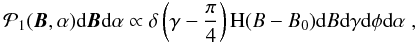
has been modeled as a slightly-modified uniform distribution, expressed as  (3)which
gives the probability of finding a magnetic field vector B
whose module is between B and B + dB,
whose inclination (with respect to the observer’s line-of-sight) is between
γ and γ + dγ, and whose azimuth (in the
plane perpendicular to the observer’s line-of-sight) is between φ and
φ + dφ. On the right-hand-side of this equation, the
term H(B − B0) also refers to the complementary
Heaviside function
(3)which
gives the probability of finding a magnetic field vector B
whose module is between B and B + dB,
whose inclination (with respect to the observer’s line-of-sight) is between
γ and γ + dγ, and whose azimuth (in the
plane perpendicular to the observer’s line-of-sight) is between φ and
φ + dφ. On the right-hand-side of this equation, the
term H(B − B0) also refers to the complementary
Heaviside function  (4)where
B0 is taken as B0 = 200 G in order
to make our experiment representative of weak field regions in the solar surface. In
addition to the value of B0, we do not make any further attempts
to employ a more realistic model for the solar internetwork since our aim is not to
investigate particular distribution functions, but rather to study the effect of the
inversion, photon noise and selection criteria in the inference of the magnetic field vector
in a general way. We note that in Eq. (3) we
employ a proportionality symbol because the normalization to one is done on
(4)where
B0 is taken as B0 = 200 G in order
to make our experiment representative of weak field regions in the solar surface. In
addition to the value of B0, we do not make any further attempts
to employ a more realistic model for the solar internetwork since our aim is not to
investigate particular distribution functions, but rather to study the effect of the
inversion, photon noise and selection criteria in the inference of the magnetic field vector
in a general way. We note that in Eq. (3) we
employ a proportionality symbol because the normalization to one is done on
 (Eq. (2)) instead of
 .
.
Once we have the probability distribution function given by Eqs. (2)–(4), we solve the radiative transfer equation in order to create a large database (=2 × 10⁶) of synthetic/theoretical Stokes profiles of the Fe I 6302.5 Å (geff = 2.5) spectral line. The effective Landé factor of the atomic transition calculated under the LS coupling scheme is indicated by geff. The Stokes profiles are synthesized with the VFISV (Very Fast Inversion of the Stokes Vector) inversion code of Borrero et al. (2011). To these profiles, photon noise is added as a normally distributed random variable with a standard deviation of σ = 10-3,3 × 10⁻⁴. These two values mimic the noise levels of maps A and C in Borrero & Kobel (2011). Once the noise is added, the resulting Stokes profiles are taken as real observations and inverted in order to retrieve the original atmospheric parameters X. This step is described in the next section.
3. Inversions of synthetic Stokes profiles
The Stokes profiles for Fe I 6302.5 Å synthesized in the previous section are now inverted with the same VFISV code, but now running in inversion mode instead of synthesis mode. At the start, VFISV solves the radiative transfer equation for polarized light in the Milne-Eddington (ME) approximation using a set of initial values for the physical parameters: X0. The solution of the radiative transfer equation yields theoretical or synthetic Stokes profiles that are compared to the ones synthesized in the previous section (those where photon noise had been added). The initial values of X0 are then iteratively modified until the best possible fit between the theoretical/synthetic and observed Stokes vector is reached. The final Xf that achieves the best fit is then assumed to be the real one present in the solar atmosphere. In this work we will focus mainly on the magnetic field vector B and magnetic filling factor α. For more details about how the inversion is performed, additional free parameters of the inversion, and treatment of the filling factor, we refer the reader to Borrero et al. (2011) and Borrero & Kobel (2011; Paper I). We note that, since we are using the same type of atmospheric model in the synthesis and inversion (ME atmospheres), the experiments carried out in this paper do not address the systematic errors introduced by the choice of the wrong atmospheric model, such as those introduced when inverting asymmetric Stokes profiles using a ME atmospheric model1.
Once B, γ, φ and α had been retrieved from each Stokes profiles of the original database, we applied two different selection criteria. In the first criteria, we select for the analysis profiles in the database where the maximum of the absolute value (for all wavelengths) in any of the polarization signals (Stokes Q, U, or V) is larger than 4.5 times the noise level max|Q(λ),U(λ),V(λ)| ≥ 4.5σ. This is equivalent to selecting pixels where the signal-to-noise ratio (S/R) in the polarization profiles is 4.5 or better, i.e., S/R ≥ 4.5. Hereafter we refer to this criteria as S/Rquv. In the second criteria we select those profiles within the database where the maximum of the absolute value (for all wavelengths) in the linear polarization signals (Stokes Q, U) is larger than 4.5 times the noise level max|Q(λ),U(λ)| ≥ 4.5σ. This criteria will be referred to as S/Rqu.
The reason behind the choice of these two different selection criteria is the following. The first criterion (selection of profiles where S/Rquv ≥ 4.5) was adopted so we can draw parallelisms with both the results presented in Paper I and Orozco Suárez et al. (2007a, 2007b). Owing to the intrinsic amplitude of Stokes Q, U, and V, this criterion selects mostly pixels where only the circular polarization V possesses a S/R ≥ 4.5. The actual percentages depend on the distribution of the magnetic field vector and the level of noise. For instance, taking a uniform distribution of B, γ, and φ (Eq. (3)) and considering a noise-level of σ = 10-3, only 21.2% of the profiles selected with the S/Rquv-criterion possess linear polarization signals (Stokes Q and U) with peak-values above 4.5σ. In the remaining 78.8% of the profiles, only Stokes V is above 4.5σ. The 21.2% increases up to 39.1% when considering a noise level of σ = 3 × 10⁻⁴. In Paper I, the maps that had equivalent levels of noise featured different percentages of profiles: in the map with σ = 10-3, only about 8.8% of the profiles selected with the S/Rquv-criterion had linear polarization profiles above 4.5σ. This number increased to 38.8% in the map with σ = 3 × 10⁻⁴. As already demonstrated in that paper (see also Martínez González et al. 2011), the inversion of profiles selected with the S/Rquv-criterion yields values for the inclination of the magnetic field vector, γ, that are largely overestimated. This happens because most of the Stokes profiles have linear polarization signals that are either below or close to the noise level. This effect decreases as the noise in the polarization profiles goes down so that the linear polarization signal rises above the noise. However, since both Stokes Q and U remain below 10-4 for transverse fields up to B⊥ ≈ 20−30 G, the overestimation in the inclination remains significant even at such low levels of noise.
In Paper I, we proposed, as an alternative solution, selecting for the inversion only pixels where the peak in the Q or U signals is at least 4.5 times higher than the noise i.e., where the S/R is higher than 4.5 in linear polarization. We also followed this approach in applying the second criterion (see also Asensio Ramos 2009). In Paper I, we anticipated that this approach has the advantage of retrieving more trustworthy values of γ, B⊥, and B but we did not quantify it.
With the results from the selected profiles using the aforementioned selection criteria, we constructed histograms for the magnetic field strength B, the inclination of the magnetic field vector with respect to the observer’s line-of-sight γ, the projection of the magnetic field vector along the observer’s line-of-sight B∥ = Bcosγ, the projection of the magnetic field vector along the perpendicular direction to the observer’s line-of-sight: B⊥ = Bsinγ; azimuthal angle of the magnetic field vector in the plane perpendicular to the observer: φ, and finally the magnetic filling factor α. Results for σ = 10-3 and S/Rquv are displayed in Fig. 1, whereas Fig. 2 presents the results for σ = 3 × 10⁻⁴ and S/Rquv. Likewise, Figs. 3 and 4 present the results for these same levels of noise, respectively, but employing the S/Rqu selection criterion. The panels in each of these four figures correspond to the following histograms: a) the component of the magnetic field vector along the observer’s line-of-sight B∥; b) the component of the magnetic field vector perpendicular the observer’s line-of-sight B⊥; c) the module of the magnetic field vector B; d) the inclination of the magnetic field vector with respect to the observer’s line-of-sight γ; e) the azimuthal angle of the magnetic field vector in the plane perpendicular to the observer’s line-of-sight φ; and finally f)-panels for the magnetic filling factor α. In all panels, solid-black lines represent the initial distribution employed in the synthesis of the Stokes profiles (see Eqs. (2)−(4)) including all 2 × 10⁶ Stokes profiles of the distribution. As required, the distributions for B, γ, φ, and α are uniform (equal probabilities). We note that this is not the case for B∥ = Bcosγ and B⊥ = Bsinγ because the cosine and sine functions introduce non-uniformities in the distribution. In addition, dashed-black lines represent the original distribution of the physical parameters but considering only the profiles that are selected with corresponding selection criteria, namely S/Rquv in Figs. 1, 2, and S/Rqu in Figs. 3, 4. Finally, the solid-red lines present the distributions inferred from the inversion of the Stokes profiles but employing the same Stokes profiles that were used to construct the dashed-black histograms. In the following we comment on some general features that will assist us in interpreting our results:
-
The area under the solid-black curve is always one, while the areaunder the dashed-black and solid-red curves are both normalizedto the quotient of the number of profiles selected with eachparticular criteria and the total number of profiles synthesized(2 × 10⁶). Therefore, one can interpret the difference between the solid-black and dashed-black curves as the loss of information caused by selection criterion, whereas the differences between dashed-black and solid-red are caused by the inversion algorithm.
-
If the solid-red curve lies below the dash-black one for a given interval of the physical parameter (e.g. Δγ), it means that the number of Stokes profiles that were synthesized employing that range of values (e.g. Δγ) are underestimated by the inversion. Likewise, whenever the solid-red curve lies above the dash-black one for a given interval, the inversion overestimates the number of Stokes profiles that were synthesized employing the range of values of the physical parameter given by the same interval.
-
The area under the dashed-black lines in each panel increases as the noise level decreases. This can be realized by comparing Fig. 1 (σ = 10-3) with Fig. 2 (σ = 3 × 10⁻⁴), and also comparing Fig. 3 (σ = 10-3) with Fig. 4 (σ = 3 × 10⁻⁴). This happens as a consequence of a larger number of Stokes profiles fulfilling the requirement imposed by a given selection criterion when the noise is reduced. Since the S/Rqu is more stringent than S/Rquv (because linear polarization signals are usually much weaker than the circular polarization signals), the area under the dashed-black curves is of course much larger in Figs. 1, 2 than Figs. 3, 4.
 |
Fig. 1 Results of the numerical experiment of the synthesis and inversion of Stokes profiles. The level noise added is σ = 10-3. Solid-black lines indicate the original distributions employed in the synthesis of 2 × 10⁶ Stokes profiles (Eq. (3)). Dashed lines show the distributions obtained employing only the Stokes profiles that are selected with the S/Rquv-criterion. The red lines display the distributions obtained from the inversion of the selected profiles: a) the absolute value of the component of the magnetic field vector that is parallel to the observer’s line-of-sight |B∥| = |Bcosγ|; b) the component of the magnetic field vector that is perpendicular to the observer’s line-of-sight B⊥ = Bsinγ; c) the magnetic field strength or module of the magnetic field vector B; d) the inclination of the magnetic field vector with respect to the observer’s line-of-sight γ; e) the azimuthal angle of the magnetic field vector on the plane that is perpendicular to the observer’s line-of-sight φ; f) the magnetic filling factor α. In all panels, the dashed-black and solid-red curves are normalized to the quotient of the number of profiles selected with each particular criteria to the total number of profiles synthesized (2 × 10⁶). |
4. Discussion
We now discuss qualitatively the effects of photon noise and selection criteria for each
physical parameter individually. We first introduce the approximate dependences of the
Stokes profiles on the three spherical coordinates of the magnetic field vector
(B, γ, φ) and the magnetic filling
factor α, in the weak field approximation (Landi Degl’Innocenti 1992) 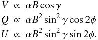 (5)
(5)
4.1. Line-of-sight component of the magnetic field: B∥
As mentioned in the previous section, the S/Rquv-criterion selects a portion of the initial Stokes profiles (dashed-black lines in Figs. 1a, 2a) that more closely resembles the original B∥ distribution (solid-black lines) than profiles selected by the S/Rqu-criterion (dashed-black lines in Figs. 3a, 4a). This is because the S/Rquv-criterion selects a much larger sample of Stokes profiles than S/Rqu, hence the distribution obtained with the former criterion must more closely resemble the original distribution employed to construct the database of Stokes profiles (solid-black lines).
We also note that the distribution of the component of the magnetic field vector along the observer’s line-of-sight B∥ is very accurately retrieved by the inversion in all instances, regardless of the selection criterion and either of the noise levels (see Figs. 1a–4a). This conclusion is reached from the fact that solid-red lines coincide almost perfectly with the dashed-black lines in all figures. In addition, the solid-red curves shift towards lower values of B∥ as the noise decreases, which indicates that lower levels of noise allow us to correctly infer smaller values of the line-of-sight component of the magnetic field.
4.2. Transverse component of the magnetic field: B⊥
For the same reason given above in the case of B∥, the S/Rquv-criterion selects a portion of the initial Stokes profiles (dashed-black lines in Figs. 1b–2b) that resembles much more closely the original B⊥ distribution (solid-black lines) than profiles selected by the S/Rqu-criterion (dashed-black lines in Figs. 3b–4b). In addition, the distribution obtained with the S/Rqu-criterion mostly provides information about the large values of the transverse component of the magnetic field (B⊥ ≈ 100−150 G), whereas the S/Rquv-criterion also selects profiles arising from weak transverse magnetic fields (B⊥ ≲ 50 G). The reason for this is that much larger values of B⊥ are needed to produce linear polarization profiles above the 4.5σ-level.
The inversion code very reliably retrieves the distribution of
B⊥ employing the
S/Rqu-criterion: we note
the almost perfect match between the solid-red curves and dashed-black ones in Figs. 3b–4b. However, this
is clearly not the case for the
S/Rquv-criterion, since
here the inversion underestimates the original distribution in the region where
B⊥ ≲ 25−40 G (depending on the noise), but overestimates
it in the region above this threshold. It is also noteworthy that the results from the
inversion of the Stokes profiles selected with the
S/Rquv-criterion show a
Maxwellian-like distribution, where the peak appears progressively at lower values of
B⊥ as the noise decreases:
 G
(Fig. 1b; σ = 10-3) and
G
(Fig. 1b; σ = 10-3) and
 G
(Fig. 2b;
σ = 3 × 10⁻⁴). This is a consequence of having a higher
sensitivity for lower levels of noise.
G
(Fig. 2b;
σ = 3 × 10⁻⁴). This is a consequence of having a higher
sensitivity for lower levels of noise.
4.3. Total magnetic field strength: B
Since  ,
and since the inversion of Stokes profiles retrieves very reliable distributions for
B∥, any mismatch between the original distributions of
B (dashed-black) and the inferred ones (solid-blue) in Figs. 1c–4c, can be
attributed to the same issues as the inference of B⊥ (see
above). In particular, as for B⊥, the
S/Rqu-criteria allows us
to retrieve the distribution of the module of the magnetic field vector B
reliably, while the
S/Rquv-criteria
underestimates the real distribution for values B ≲ 35−70 G (depending
on the noise) but overestimates it above this threshold (solid-blue lines in Figs. 1c and 2c).
,
and since the inversion of Stokes profiles retrieves very reliable distributions for
B∥, any mismatch between the original distributions of
B (dashed-black) and the inferred ones (solid-blue) in Figs. 1c–4c, can be
attributed to the same issues as the inference of B⊥ (see
above). In particular, as for B⊥, the
S/Rqu-criteria allows us
to retrieve the distribution of the module of the magnetic field vector B
reliably, while the
S/Rquv-criteria
underestimates the real distribution for values B ≲ 35−70 G (depending
on the noise) but overestimates it above this threshold (solid-blue lines in Figs. 1c and 2c).
4.4. Inclination of the magnetic field vector: γ
As happens with B∥ and B⊥, the S/Rquv-criterion selects a set of Stokes profiles (dashed-black lines in Figs. 1d–2d) that are more representative of the initial uniform distribution in γ (solid-black lines) than the Stokes profiles chosen with the S/Rqu-criteria (dashed-black lines in Figs. 3d–4d). The S/Rquv-criterion selects all sorts of inclinations, with a slight preference for more longitudinal magnetic fields. The S/Rqu-criterion selects however only highly inclined fields (γ → 90°). This happens because for weak magnetic fields, the only way to have linear polarization signals above the 4.5σ-level is for these magnetic fields to be highly inclined. This can also be understood in terms of the kind of distributions obtained in B∥ and in B⊥ (panels a) and b), respectively) by each selection criteria and remembering that γ = tan-1(B⊥/B∥).
By comparing the dashed-black and solid-red lines in Figs. 1d–4d, we can conclude that the inversions of the Stokes profiles selected with the S/Rquv-criterion yields a distribution of γ that is underestimated for more longitudinal magnetic fields, but overestimated for more transverse ones. We note that the turning point between the underestimation of vertical magnetic fields and the overestimation of horizontal ones occurs at lower values of γ as the noise decreases: γ ≃ 22° for σ = 10-3 but only at γ ≃ 17° for σ = 3 × 10⁻⁴. Interestingly, the probability distribution function around γ = 90° (where magnetic fields are perpendicular to the line-of-sight) is reliably inferred with this criterion. Altogether, these findings confirm our previous results (see Paper I), for which we concluded that the inversion of the Stokes profiles obtained with the S/Rquv-criterion will correctly infer very inclined magnetic fields, whenever these are present, but unfortunately also interpret as very inclined magnetic fields those that are mostly aligned with the observer’s line-of-sight. In contrast, the inversion of pixels selected with the S/Rqu-criterion retrieves almost perfectly the distribution of the selected pixels, as can be seen by comparing the dashed-black and solid-red curves in Figs. 3d–4d.
4.5. Azimuth of the magnetic field vector: φ
Here, both the S/Rquv and S/Rqu-criteria select a set of Stokes profiles that are representative of the original uniform azimuthal distribution of the magnetic field vector, φ, as the selected distributions are also very close to uniform (compare the dashed-black and solid-black lines in Figs. 1e–4e).
Remarkably, the inversion of the selected Stokes profiles for both values of the photon noise, σ, and both selection criteria is able to retrieve the original distribution of the selected profiles, as the solid-red lines in Figs. 1e–4e match the dashed-black ones. To a first approximation (Auer et al. 1977; Jeferries & Mickey 1991), the azimuthal angle of the magnetic field vector is given by φ = (1/2)tan-1(U/Q). Thus, that the inversion of the Stokes profiles selected with the S/Rquv-criterion also retrieves the correct distribution for φ comes as a rather surprising result, since here most of the selected Stokes Q and U profiles are below the 4.5σ-level (see Sect. 3). We address this particular point in Sect. 5.
4.6. Magnetic filling factor: α
In the case of the magnetic filling factor α, neither the S/Rquv nor the S/Rqu criteria (dashed-black lines in Figs. 1f–4f) are able to recover correctly the original uniform distribution (solid-black lines). In particular, most of the Stokes profiles arising from low values of the filling factor, α ≲ 0.4, are neglected by both selection criteria. This is because the polarization signals scale linearly with α (see Eq. (5)) and therefore, small values of the magnetic filling factor yield polarization signals that are below the threshold employed in the selection. The situation is aggravated in the case of S/Rqu (Figs. 3, 4), where even larger values of α are needed owing to Stokes Q and U being intrinsically smaller than Stokes V.
As far as the inversion is concerned, it is clear that the distribution of the magnetic filling factor of the selected profiles is very well-retrieved (solid-red lines in Figs. 1f–4f) for both noise levels and when employing both selection criteria. Interestingly, as happened with γ (although to a much smaller extent), the inversion code slightly overestimates the selected distribution (dashed-black) for α ≲ 0.5, but underestimates it above this value.
We have so far only discussed the ability of the inversion code to retrieve the correct distribution for the magnetic parameters (three components of the magnetic field vector and filling factor). Although this is clearly an important question, it does not provide much information about the reliability of the inversion in individual cases. To address this point, we display in circles in Fig. 5, the mean value of the differences between the original physical parameters of the selected Stokes profiles and the inferred ones through the inversion Xsel − Xinv. These are denoted as ΔXi, with Xi being any of the components of X in Eq. (1), which we refer to as bias in Xi. In addition to this, we also plot the standard deviation around the mean in the inference of the physical parameters as the dashed-color lines, which we refer to as σx (not to be confused with the photon noise σ). For a physical parameter to be well-constrained, it is important that the mean is centered around zero (otherwise a systematic bias occurs) and that the standard deviation is small.
We note that the size of the intervals in which the bias and standard deviation are calculated is not constant. This happens as a consequence of the lack of profiles in certain ranges. For instance, the S/Rqu criterion barely selects profiles arising from a magnetic field vector where B⊥ < 50 G (see red and yellow circles in Figs. 3b–4b). This makes it necessary to increase the interval of B⊥ (around this range) so that a sufficient number of profiles can be employed to obtain a statistically meaningful ΔB⊥ and σB⊥ (see green and yellow circles in Fig. 5b). This is not needed as often in the S/Rquv-criterion because it selects many more profiles than the S/Rqu-criterion (blue and red circles in Fig. 5b).
By inspection of Fig. 5, we note that, for the same level of noise and with the exception of the magnetic filling factor α, the standard deviation in the retrieval of the physical parameters is always much smaller when employing the S/Rqu-criterion than the S/Rquv-criterion. By comparing the standard deviations with different levels of photon noise, we realize that for most physical parameters, the improvement achieved by a decrease in the photon noise (from σ = 10-3 to 3 × 10⁻⁴) is smaller than the improvement achieved by using the S/Rqu instead of the S/Rquv-criterion. This, generally makes the dashed-green curves (σ = 10-3 and S/Rqu-criterion) lie below the red-dashed ones (σ = 3 × 10⁻⁴ and S/Rquv-criterion). Interestingly, this does not apply to all physical parameters: in the case of B∥ and α, the photon noise plays a more important role than the selection criteria itself, as the red curves lie below the green ones. The relative importances of the selection criteria and the photon noise logically depends on the values of the noise considered, thus we cannot conclude that in general the former is more important than the latter (or the other way around) for some particular physical parameter.
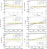 |
Fig. 5 Mean values of the differences between the original physical parameters and the inferred values (ΔXi; circles) and standard deviations around the mean (dashed lines; σx): (panel-a)) ΔB∥ and σB∥ as a function of B∥; (panel-b)) ΔB⊥ and σB⊥ as a function of B⊥; (panel-c)) ΔB and σB and a function of B; (panel-d)) Δγ and σγ as a function of γ; (panel-e)) Δφ and σφ as a function of γ; and finally, (panel-f)) Δα and σα as a function of α. Blue shows the results obtained from a photon-noise level of σ = 10-3 and selection criterion S/Rquv (from Fig. 1); red represents σ = 3 × 10⁻⁴ and S/Rquv (from Fig. 2); green is for σ = 10-3 and S/Rqu (from Fig. 3); and yellow is for σ = 3 × 10⁻⁴ and S/Rqu (from Fig. 4). |
We now discuss the errors in the case of the
S/Rquv-criterion. Here,
the retrieval of B⊥ (blue and red colors in Fig. 5b) has a large systematic bias towards
 , such as
ΔB⊥ < −75 G, for
, such as
ΔB⊥ < −75 G, for
 G. Furthermore, in this
same region, the standard deviation is as large as
σB⊥ ≈ 20−50 G. These
numbers decrease as
G. Furthermore, in this
same region, the standard deviation is as large as
σB⊥ ≈ 20−50 G. These
numbers decrease as  increases,
such that ΔB⊥ ≈ −15 G and
σB⊥ ≈ 10 G for
increases,
such that ΔB⊥ ≈ −15 G and
σB⊥ ≈ 10 G for
 G. As
happened in the case of the distributions in Figs. 1c–4c, the bias and standard deviations in
the module of the magnetic field vector B (Fig. 5c) mimic those of B⊥ (Fig. 5b). In the case of B∥
(blue and red colors in Fig. 5a), both the bias and
standard deviation are always quite small <5 G, owing to the
Stokes V profiles typically being much larger than Q and
U for the same values of B∥ and
B⊥. For the inclination of the magnetic field vector with
respect to the observer’s line-of-sight, γ (blue and red colors in
Fig. 5d), the bias is systematic towards more
inclined magnetic fields: Δγ < 0 if
γsel < 90°, but
Δγ > 0 if
γsel > 90°. The absolute
value of the bias is indeed larger for magnetic fields aligned with the observer’s
line-of-sight, where |Δγ| ≈ 30−40° if
γsel ≈ 0,180°. Interestingly,
the bias decreases as the magnetic field vector becomes more perpendicular to the
line-of-sight, i.e., Δγ = 0 for
γsel ≈ 90°. The behavior of
σγ is very similar (at all values) to
that of the absolute values of bias |Δγ|. That the bias and standard
deviation decrease as γ → 90° indicates that when the magnetic
field vector is not completely aligned with the observer’s line-of-sight, the signal that
appears in Q and U helps the inversion code to extract
some information about the inclination of the magnetic field vector. This inference is
however negatively affected by the photon noise systematically overestimating
γ. This agrees with our results in Paper I, where we found that it was
impossible to distinguish between a vertical and horizontal magnetic-field vector when
Stokes Q and U are below the
4.5σ-level. Figure 5e displays
Δφ and σφ as a function of
γsel instead of φsel. In this
case, the bias in the determination of the azimuthal angle of the magnetic field vector is
almost negligible for all possible values of γsel, where
Δφ ≈ 0°. However, the standard deviation is large
(σφ ≈ 40−50°) when the
magnetic field vector is aligned with the observer’s line-of-sight
(γ → 0,180°), but decreases as the magnetic
field vector becomes more and more inclined with respect to the observer’s line-of-sight
(γ → 90°). This happens as a consequence of the linear
polarization profiles vanishing when the magnetic field becomes aligned with the observer
such that Q,U ∝ sin2γ (see Eq. (5)).
G. As
happened in the case of the distributions in Figs. 1c–4c, the bias and standard deviations in
the module of the magnetic field vector B (Fig. 5c) mimic those of B⊥ (Fig. 5b). In the case of B∥
(blue and red colors in Fig. 5a), both the bias and
standard deviation are always quite small <5 G, owing to the
Stokes V profiles typically being much larger than Q and
U for the same values of B∥ and
B⊥. For the inclination of the magnetic field vector with
respect to the observer’s line-of-sight, γ (blue and red colors in
Fig. 5d), the bias is systematic towards more
inclined magnetic fields: Δγ < 0 if
γsel < 90°, but
Δγ > 0 if
γsel > 90°. The absolute
value of the bias is indeed larger for magnetic fields aligned with the observer’s
line-of-sight, where |Δγ| ≈ 30−40° if
γsel ≈ 0,180°. Interestingly,
the bias decreases as the magnetic field vector becomes more perpendicular to the
line-of-sight, i.e., Δγ = 0 for
γsel ≈ 90°. The behavior of
σγ is very similar (at all values) to
that of the absolute values of bias |Δγ|. That the bias and standard
deviation decrease as γ → 90° indicates that when the magnetic
field vector is not completely aligned with the observer’s line-of-sight, the signal that
appears in Q and U helps the inversion code to extract
some information about the inclination of the magnetic field vector. This inference is
however negatively affected by the photon noise systematically overestimating
γ. This agrees with our results in Paper I, where we found that it was
impossible to distinguish between a vertical and horizontal magnetic-field vector when
Stokes Q and U are below the
4.5σ-level. Figure 5e displays
Δφ and σφ as a function of
γsel instead of φsel. In this
case, the bias in the determination of the azimuthal angle of the magnetic field vector is
almost negligible for all possible values of γsel, where
Δφ ≈ 0°. However, the standard deviation is large
(σφ ≈ 40−50°) when the
magnetic field vector is aligned with the observer’s line-of-sight
(γ → 0,180°), but decreases as the magnetic
field vector becomes more and more inclined with respect to the observer’s line-of-sight
(γ → 90°). This happens as a consequence of the linear
polarization profiles vanishing when the magnetic field becomes aligned with the observer
such that Q,U ∝ sin2γ (see Eq. (5)).
Compared to the S/Rquv-criterion, there is no bias in the retrieval of all parameters (except for the magnetic filling factor) when employing the S/Rqu-criterion ΔXi → 0. In addition, the standard deviation in the retrieval of the physical parameters, σx, greatly decreases when employing the S/Rqu-criterion, as indicated by the green and yellow colors in Fig. 5. With this criterion ΔB⊥ ≈ 0 G and σB⊥ ≈ 10 G, even for B⊥ < 50 G. The retrieval of B∥ also improves, (such that σB∥ < 3 G) from that achieved with the S/Rquv-criterion. Finally, this translates into smaller standard deviations for B, γ, and φ: σB < 5 G, σγ < 2°, and σφ < 2°.
5. Can inversion codes retrieve the distribution of the orientation of the magnetic field vector from correlations within the noise ?
5.1. Azimuth of the magnetic field vector: φ
In Sect. 4.5, we have seen that the retrieved
distribution of the azimuthal angle of the magnetic field vector on the plane that is
perpendicular to the observer’s line-of-sight (φ) matches excellently
well the original uniform distribution for the selected pixels. In the case of the
S/Rquv-criterion, this
seems counter-intuitive since many of the selected Stokes profiles only have sufficient
signal in Stokes V, while Q and U are
usually dominated by photon noise. One possible explanation for this is that the inversion
does not properly infer φ but instead yields a random distribution of
values owing to the lack of information in the linear polarization profiles. If this
distribution happens to be uniformly distributed, then the inferred distribution of
azimuths matches the original one, even if the inversion fails for each Stokes vector
individually. The second explanation is that, given that the number of profiles with large
enough signals in Stokes Q and U is non-negligible, the
inversion indeed properly retrieves φ. In particular, in Sect. 3 we mentioned that 21.2%
(σ = 10-3) and 39.2%
(σ = 3 × 10⁻⁴) of the profiles selected with the
S/Rquv-criteron, had
linear polarization signals above the 4.5σ-level. A final possible
explanation is that the inversion is able to retrieve the correct values of
φ even when Stokes Q and U are
dominated by noise. This could happen if the hidden signal introduces a sufficiently
strong correlation in the noise, such that the minimization process can properly retrieve
the azimuth of the magnetic field vector. To investigate which of these three
possibilities are responsible for our results in Sect. 4, we repeated the synthesis (Sect. 2) and
inversion experiments of the spectral line Fe I 6302.5 Å, but employing the probability
distribution function 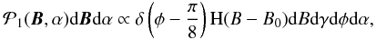 (6)which
is very similar to Eq. (3) with the
exception that the distribution of the azimuthal angle is now a δ-Dirac
centered at 22.5° = π/8 rad. This value is
chosen such that
Q ∝ sin2γcos2φ, and
U ∝ sin2γsin2φ, have the
same amplitudes (see Eq. (5)). The
distribution given by Eq. (6) is employed
to produce synthetic Stokes profiles, which are then inverted after adding photon noise
with levels of σ = 10-3 and 3 × 10⁻⁴. The resulting
distributions, for both levels of noise and both selection criteria
(S/Rquv and
S/Rqu), are shown in
Fig. 6.
(6)which
is very similar to Eq. (3) with the
exception that the distribution of the azimuthal angle is now a δ-Dirac
centered at 22.5° = π/8 rad. This value is
chosen such that
Q ∝ sin2γcos2φ, and
U ∝ sin2γsin2φ, have the
same amplitudes (see Eq. (5)). The
distribution given by Eq. (6) is employed
to produce synthetic Stokes profiles, which are then inverted after adding photon noise
with levels of σ = 10-3 and 3 × 10⁻⁴. The resulting
distributions, for both levels of noise and both selection criteria
(S/Rquv and
S/Rqu), are shown in
Fig. 6.
Figure 6 shows that, on the one hand, the S/Rquv-criterion (solid lines) has an almost uniform background distribution. This is caused by the inversion of Stokes profiles whose linear polarization signals are so weak that they carry no information about the azimuth, thus the inversion retrieves random results that happen to be uniformly distributed. We know this because this background uniform field disappears if we apply the S/Rqu-criterion (dashed lines), which selects only Stokes Q and U profiles that are 4.5 times above the noise level. This is therefore one of the reasons for the excellent results in Figs. 1e–2e.
In Fig. 6, the S/Rquv-criterion also features (superimposed on the uniform background distribution) a clear reminiscent signature of the original δ(φ − π/8) distribution (indicated by the vertical black arrow). This indicates that the inversion code is able to retrieve, to some extent, information about the azimuthal angle of the magnetic field vector. However, we still do not know whether φ is correctly retrieved in only 21.2/39.2% (σ = 10-3,3 × 10⁻⁴, respectively) of the Stokes profiles that have sufficient signal in the linear polarization or, whether the inversion can properly infer φ even when the linear polarization signals are below the 4.5σ-level. To answer this question, we devised a third selection criterion, S/Rno−qu, for which we selected all profiles where the linear polarization signals were below the 4.5σ-level. The distribution of φ obtained with this criterion (dotted-dashed lines in Fig. 6) shows an almost uniform distribution, with a far smaller peak at φ = π/8 than before. This indicates that when the signals are dominated by noise, the correlation hidden below the noise does not provide sufficient information about the azimuthal angle of the magnetic field vector.
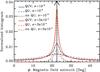 |
Fig. 6 Histograms of the inferred azimuthal angle of the magnetic field vector, φ, when employing Eq. (6) in the synthesis of Stokes profiles. The original distribution δ(φ − π/8) is indicated by the vertical black arrow located at φ = 22.5°. The inferred histograms using S/Rquv, S/Rqu, and S/Rno−qu criteria are indicated by the solid, dashed, and dotted-dashed lines, respectively. Blue curves are obtained with a photon noise σ = 10-3, whereas red ones correspond to σ = 3 × 10⁻⁴. |
5.2. Inclination of the magnetic field vector: γ
In Paper I, we demonstrated that a magnetic field vector that is aligned with the
observer’s line-of-sight (γ = 0,180°) can be
easily confused with a more perpendicular one (γ ≈ 90°) owing
to the effect of the photon noise. In that experiment, the signals in the linear
polarization were solely due to the photon noise. We did not study whether the inversion
code could retrieve useful information about γ from the Stokes
Q and U profiles that, in spite of being below the
4.5σ-level, introduce a correlation within the noise. To study this
possibility, we carry out a similar experiment to the one we have performed in Sect. 5.1, but focusing instead on the inclination of the
magnetic field vector with respect to the observer’s line-of-sight γ. To
this end, we prescribe a theoretical distribution of the magnetic field vector in the form
 (7)which
is identical to the distribution in Eq. (6)
but where the roles of φ and γ are exchanged. That is,
the distribution of the azimuth is now uniform and the distribution of the inclination is
now a δ-Dirac function centered at
γ = 45° = π/4 rad, which
is chosen to ensure that
B∥ = Bcosγ and
B⊥ = Bsinγ (see
Eq. (5)) are equal. As we did in
Sect. 5.2, we add to the resulting Stokes profiles
synthesized with Eq. (7) photon noise with
the values σ = 10-3,3 × 10⁻⁴. We
also apply the three selection criteria mentioned above of
S/Rquv,
S/Rqu, and
S/Rno−qu. The inferred
histograms of γ are displayed in Fig. 7.
(7)which
is identical to the distribution in Eq. (6)
but where the roles of φ and γ are exchanged. That is,
the distribution of the azimuth is now uniform and the distribution of the inclination is
now a δ-Dirac function centered at
γ = 45° = π/4 rad, which
is chosen to ensure that
B∥ = Bcosγ and
B⊥ = Bsinγ (see
Eq. (5)) are equal. As we did in
Sect. 5.2, we add to the resulting Stokes profiles
synthesized with Eq. (7) photon noise with
the values σ = 10-3,3 × 10⁻⁴. We
also apply the three selection criteria mentioned above of
S/Rquv,
S/Rqu, and
S/Rno−qu. The inferred
histograms of γ are displayed in Fig. 7.
With the first selection criterion, S/Rquv, we realize that the inversion code retrieves a distribution of γ (solid lines in Fig. 7) with a clear peak at the original value of γ = 45°. This distribution has however an extended asymmetric tail towards higher values of γ. This indicates that there is a tendency to retrieve field that are more inclined than they originally are, as a consequence of inverting Stokes profiles where Q and U are not 4.5 times above the noise level. This becomes clear when we consider the S/Rqu-criterion (dashed lines in Fig. 7), which ensures that the linear polarization profiles are above the 4.5σ-level, since in this case the tail towards larger values of γ disappears. What are the properties of the peak at γ = 45° obtained with the S/Rquv-criterion? Is it a consequence of the inversion code being able to properly retrieve the inclination from the weak linear-polarization signals that are below the noise level but introduce a correlation into the noise? Or does the peak contain, as in the case of φ (Sect. 5.1) and since a large portion of the Stokes profiles were selected with the S/Rquv-criterion, strong linear-polarization signals? This can be answered by the S/Rno−qu-criterion, which only selects Stokes profiles for which Stokes Q and U are below the 4.5σ-level (see dotted-dashed lines in Fig. 7). This selection criteria shows an even more pronounced tail towards larger values of γ than the S/Rquv-criteria. This is a consequence of many more Stokes profiles containing no information about γ owing to very noisy linear-polarization signals. However, the peak at γ = 45° does not completely disappear, which indicates that, unlike the case of φ, the inversion code is able to partially use the correlation hidden in the noise as a means of determining γ.
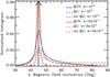 |
Fig. 7 Histograms of the inferred inclination angle of the magnetic field vector, γ, when employing Eq. (7) in the synthesis of Stokes profiles. The original distribution δ(γ − π/4) is indicated by the vertical black arrow located at φ = 55°. The inferred histograms using S/Rquv, S/Rqu, and S/Rno−qu criteria are indicated by the solid, dashed, and dotted-dashed lines, respectively. Blue curves are obtained with a photon noise σ = 10-3, whereas red ones correspond to σ = 3 × 10⁻⁴. |
We note, however, that this does not mean that the inversion code is able to retrieve the correct distribution of γ by employing the S/Rno−qu-criterion (Stokes Q and U profiles below the 4.5σ-level) when the distribution is a more general one than the δ-Dirac function employed in Eq. (7). To emphasize this statement, it suffices to point out that not even the S/Rquv-criteria, where 20−40% of the Stokes profiles have linear polarization signals above the 4.5σ-level, is able to do so (see Figs. 1d–2d). As demonstrated in Sect. 4, the only way of retrieving the original distributions of the magnetic field vector is to ensure that the linear polarization is above the 4.5σ-level, that is, to apply the S/Rqu-criterion.
6. Conclusions
We have carried out several numerical experiments in which a large number of Stokes profiles have been synthesized using uniform distributions of the three components of the magnetic field vector B, γ, and φ, and the magnetic filling factor α (Eq. (3)). To these Stokes profiles, we have added photon noise to two different levels of σ = 10-3, and σ = 3 × 10⁻⁴. We have then inverted these profiles in order to retrieve the original distributions employed in the synthesis. This has been done in two different ways. In the first one, we have selected the pixels where the S/R ratio in any of the polarization signals (circular or linear) are equal to or larger than 4.5, the so-calld S/Rquv-criterion. In the second case, we have selected the pixels where the S/R ratio in the linear polarization signals is equal to or larger than 4.5, which is the S/Rqu-criterion. The former criterion, S/Rquv, selects Stokes profiles that arise from all possible ranges of B, γ, and φ (dashed-black curves in Figs. 1, 2), whereas the S/Rqu-criterion selects Stokes profiles that arise from highly inclined magnetic fields (dashed-black curves in Figs. 3, 4).
In addition, we have demonstrated (see Sect. 4) that the S/Rqu-criterion can recover, with much larger reliability than S/Rquv, the original distributions of the three components of the magnetic field vector from the selected profiles. In particular, the latter criterion clearly overestimates the inclination (with respect to the observer’s line-of-sight) of the magnetic field vector γ (solid-red lines in Figs. 1d−2d), and therefore also overestimates the component of the magnetic field that is perpendicular to the observer’s line-of-sight, B⊥ (solid-red lines in Figs. 1b−2b). To avoid these systematic errors, we propose employing instead the S/Rqu-criterion, which allows the correct distribution of B⊥ and γ (solid-red lines in Figs. 3b,d−4b,d) from the selected profiles to be retrieved. Unfortunately, as mentioned above, the S/Rqu-criterion systematically selects the Stokes profiles where the magnetic field vector is already rather inclined, and thus ends up having the same sort of bias as the S/Rquv-criterion. It seems therefore that the only way around this problem is to decrease the photon noise to a sufficiently low level that the vast majority of profiles have a S/R ratio larger than 4.5 in the linear polarization profiles. In this way, the selected Stokes profiles would arise from magnetic fields that are representative of the real distribution. It is important to bear in mind that the overestimation of γ and B⊥ is a result that does not depend on the probability distribution function employed in our tests (Eq. (3)).
We have also studied the ability of the inversion code to retrieve the angular distribution of the magnetic field vector (γ and φ), even when the Stokes Q and U profiles are below the 4.5σ-level (Sect. 5). In this case, we employed initial distributions of φ and γ featuring δ-Dirac functions. We found that the correlation introduced into the noise by these signals does not help us to retrieve the correct azimuthal angle φ. Instead of the original δ-function, the inversion code yields a random distribution of azimuthal angles that are uniformly distributed (Fig. 6). In the case of the inclination of the magnetic field vector γ, the inversion code is able to partially retrieve the δ-function from the weak signals below the noise (Fig. 7). However, this is not the case when employing more general distributions, in which case the aforementioned systematic overestimation of γ, dominates the inferred distribution (cf. del Toro Iniesta et al. 2010).
We caution that in our experiments we employed only one spectral line, Fe I (geff = 2.5) 6302.5 Å, whereas in many previous studies Fe I (geff = 1.67) 6301.5 Å had also been analyzed. Employing two spectral lines would certainly somewhat improve the results from these experiments as there would be more data points available to the inversion code. However, based on the results of Orozco Suárez et al. (2010), these improvements will likely be of second order compared to the systematic errors presented in this paper.
An additional point of consideration refers to the numerical code used to infer the magnetic field vector from the inversion of the radiative transfer equation for polarized light (VFISV). This code operates, with some modifications, under a Levenberg-Marquardt non-linear minimization algorithm (Borrero et al. 2011). We cannot exclude that other numerical schemes such as genetic (Lagg et al. 2004) or Bayesian algorithms (Asensio Ramos et al. 2008; Asensio Ramos 2009) are less affected by photon noise and therefore able to infer more accurately the distribution of the magnetic field vector.
Other sources of systematic errors that are not being considered, as they are beyond the scope of our study, are the effects of the spatial resolution, spectral resolution, etcetera. For instance, Borrero et al. (2007) carried out such a study for the particular case of the Helioseismic and Magnetic Imager (HMI) instrument.
Acknowledgments
This research has greatly benefited from discussions that were held at the International Space Science Institute (ISSI) in Bern (Switzerland) in February 2010 as part of the International Working group Extracting Information from spectropolarimetric observations: comparison of inversion codes. This work has made use of the NASA Astrophysical Data System.
References
- Asensio Ramos, A., Martínez González, M. J., López Ariste, A., TrujilloBueno, J., & Collados, M. 2007, ApJ, 659, 829 [NASA ADS] [CrossRef] [Google Scholar]
- Asensio Ramos, A., Trujillo Bueno, J., & Landi Degl’ Innocenti, E. 2008, ApJ, 683, 542 [NASA ADS] [CrossRef] [Google Scholar]
- AsensioRamos, A. 2009, ApJ, 701, 1032 [NASA ADS] [CrossRef] [Google Scholar]
- Auer, L. H., House, L. L., & Heasley, J. N. 1977, Sol. Phys., 55, 47 [NASA ADS] [CrossRef] [Google Scholar]
- Bellot Rubio, L. R. 2003, in Proc. Solar Polarization Workshop 4, eds. R. Casini, & B. W. Lites, ASP Conf. Ser., 358, 107 [Google Scholar]
- Borrero, J. M., & Kobel, P. 2011, A&A, 527, A29 (Paper I) [NASA ADS] [CrossRef] [EDP Sciences] [Google Scholar]
- Borrero, J. M., Tomczyk, S., Norton, A., et al. 2007, Sol. Phys., 240, 177 [NASA ADS] [CrossRef] [Google Scholar]
- Borrero, J. M., Tomczyk, S., Kubo, M., et al. 2011, Sol. Phys., 273, 267 [Google Scholar]
- Domínguez Cerdeña, I., Sánchez Almeida, J., & Kneer, F. 2003, ApJ, 582, 55 [Google Scholar]
- Jefferies, J. T., & Mickey, D.L 1991, ApJ, 372, 694 [NASA ADS] [CrossRef] [Google Scholar]
- Ishikawa, R., & Tsuneta, S. 2011, ApJ, 735, 74 [NASA ADS] [CrossRef] [Google Scholar]
- Martínez González, M. J., Collados, M., & Ruiz Cobo, B. 2006, A&A, 456, 1159 [NASA ADS] [CrossRef] [EDP Sciences] [Google Scholar]
- Martínez González, M., Asensio Ramos, A., López Ariste, A., & Manso-Sainz, R. 2008, A&A, 479, 229 [NASA ADS] [CrossRef] [EDP Sciences] [Google Scholar]
- Martínez González, M., Manso Sainz, R., Asensio Ramos, A., & Belluzzi, L. 2011, MNRAS, 419, 153 [Google Scholar]
- Mathys, G. 2002 in Astrophysical Spectropolarimetry, eds. J. Trujillo-Bueno, F. Moreno-Insertis, & F. Sánchez (Cambridge University Press), 101 [Google Scholar]
- Lagg, A., Woch, J., Krupp, N., & Solanki, S. K. 2004, A&A, 414, 1109 [NASA ADS] [CrossRef] [EDP Sciences] [Google Scholar]
- Landi Degl’Innocenti, E. 1992, in Solar Observations, Techniques and intepretations, eds. F. Sánchez, M. Collados, & M. Vázquez (Cambridge University Press), 71 [Google Scholar]
- Lites, B. W., Leka, K. D., Skumanich, A., Martínez-Pillet, V., & Shimuzu, T. 1996, ApJ, 460, 1019 [NASA ADS] [CrossRef] [Google Scholar]
- Lites, B. W., Socas-Navarro, H., Kubo, M., et al. 2007, PASJ, 59, 571 [Google Scholar]
- Lites, B. W., Kubo, M., Socas-Navarro, H., et al. 2008, ApJ, 672, 1237 [NASA ADS] [CrossRef] [Google Scholar]
- López Ariste, A., Martínez González, M. J., & Ramírez Vélez, J. C. 2007, A&A, 464, 351 [NASA ADS] [CrossRef] [EDP Sciences] [Google Scholar]
- Orozco Suárez, D., Bellot Rubio, L. R., del Toro Iniesta, J. C., et al. 2007a, ApJ, 670, L61 [NASA ADS] [CrossRef] [Google Scholar]
- Orozco Suárez, D., Bellot Rubio, L. R., del Toro Iniesta, J. C., et al. 2007b, PASJ, 59, 837 [Google Scholar]
- Orozco Suárez, D., Bellot Rubio, L. R., Vögler, A., & del Toro Iniesta, J. C. 2010, A&A, 518, A2 [Google Scholar]
- Ruiz Cobo, B. 2007, in Modern solar facilities – advanced solar science, eds. F. Kneer, K. G. Puschmann, & A. D. Wittmann, 287 [Google Scholar]
- Sánchez Almeida, J. 2005, A&A, 438, 727 [NASA ADS] [CrossRef] [EDP Sciences] [Google Scholar]
- Socas-Navarro, H., & Lites, B. W. 2004, ApJ, 616, 587 [NASA ADS] [CrossRef] [Google Scholar]
- Socas-Navarro, H., Borrero, J. M., Asensio Ramos, A., et al. 2008, ApJ, 674, 596 [NASA ADS] [CrossRef] [Google Scholar]
- Stenflo, J. O. 2002, in Astrophysical Spectropolarimetry, eds. J. Trujillo-Bueno, F. Moreno-Insertis, & F. Sánchez (Cambridge University Press), 55 [Google Scholar]
- del Toro Iniesta, J. C. 2003a, Astron. Nachr., 324, 383 [NASA ADS] [CrossRef] [Google Scholar]
- del Toro Iniesta, J. C. 2003b, Introduction to Spectropolarimetry (Cambridge, UK: Cambridge University Press) [Google Scholar]
- del Toro Iniesta, J. C., Orozco Suárez, D., & Bellot Rubio, L. R. 2010, ApJ, 711, 312 [NASA ADS] [CrossRef] [Google Scholar]
All Figures
|
Fig. 1 Results of the numerical experiment of the synthesis and inversion of Stokes profiles. The level noise added is σ = 10-3. Solid-black lines indicate the original distributions employed in the synthesis of 2 × 10⁶ Stokes profiles (Eq. (3)). Dashed lines show the distributions obtained employing only the Stokes profiles that are selected with the S/Rquv-criterion. The red lines display the distributions obtained from the inversion of the selected profiles: a) the absolute value of the component of the magnetic field vector that is parallel to the observer’s line-of-sight |B∥| = |Bcosγ|; b) the component of the magnetic field vector that is perpendicular to the observer’s line-of-sight B⊥ = Bsinγ; c) the magnetic field strength or module of the magnetic field vector B; d) the inclination of the magnetic field vector with respect to the observer’s line-of-sight γ; e) the azimuthal angle of the magnetic field vector on the plane that is perpendicular to the observer’s line-of-sight φ; f) the magnetic filling factor α. In all panels, the dashed-black and solid-red curves are normalized to the quotient of the number of profiles selected with each particular criteria to the total number of profiles synthesized (2 × 10⁶). |
| In the text | |
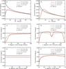 |
Fig. 2 Same as Fig. 1 but using a photon noise σ = 3 × 10⁻⁴ and the S/Rquv-criterion. |
| In the text | |
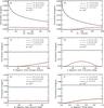 |
Fig. 3 Same as Fig. 1 but using a photon noise σ = 10-3 and the S/Rqu-criterion. |
| In the text | |
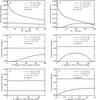 |
Fig. 4 Same as Fig. 1 but using a photon noise σ = 3 × 10⁻⁴ and the S/Rqu-criterion. |
| In the text | |
|
Fig. 5 Mean values of the differences between the original physical parameters and the inferred values (ΔXi; circles) and standard deviations around the mean (dashed lines; σx): (panel-a)) ΔB∥ and σB∥ as a function of B∥; (panel-b)) ΔB⊥ and σB⊥ as a function of B⊥; (panel-c)) ΔB and σB and a function of B; (panel-d)) Δγ and σγ as a function of γ; (panel-e)) Δφ and σφ as a function of γ; and finally, (panel-f)) Δα and σα as a function of α. Blue shows the results obtained from a photon-noise level of σ = 10-3 and selection criterion S/Rquv (from Fig. 1); red represents σ = 3 × 10⁻⁴ and S/Rquv (from Fig. 2); green is for σ = 10-3 and S/Rqu (from Fig. 3); and yellow is for σ = 3 × 10⁻⁴ and S/Rqu (from Fig. 4). |
| In the text | |
|
Fig. 6 Histograms of the inferred azimuthal angle of the magnetic field vector, φ, when employing Eq. (6) in the synthesis of Stokes profiles. The original distribution δ(φ − π/8) is indicated by the vertical black arrow located at φ = 22.5°. The inferred histograms using S/Rquv, S/Rqu, and S/Rno−qu criteria are indicated by the solid, dashed, and dotted-dashed lines, respectively. Blue curves are obtained with a photon noise σ = 10-3, whereas red ones correspond to σ = 3 × 10⁻⁴. |
| In the text | |
|
Fig. 7 Histograms of the inferred inclination angle of the magnetic field vector, γ, when employing Eq. (7) in the synthesis of Stokes profiles. The original distribution δ(γ − π/4) is indicated by the vertical black arrow located at φ = 55°. The inferred histograms using S/Rquv, S/Rqu, and S/Rno−qu criteria are indicated by the solid, dashed, and dotted-dashed lines, respectively. Blue curves are obtained with a photon noise σ = 10-3, whereas red ones correspond to σ = 3 × 10⁻⁴. |
| In the text | |
Current usage metrics show cumulative count of Article Views (full-text article views including HTML views, PDF and ePub downloads, according to the available data) and Abstracts Views on Vision4Press platform.
Data correspond to usage on the plateform after 2015. The current usage metrics is available 48-96 hours after online publication and is updated daily on week days.
Initial download of the metrics may take a while.