| Issue |
A&A
Volume 547, November 2012
|
|
|---|---|---|
| Article Number | A98 | |
| Number of page(s) | 5 | |
| Section | Cosmology (including clusters of galaxies) | |
| DOI | https://doi.org/10.1051/0004-6361/201116983 | |
| Published online | 06 November 2012 | |
Calibration biases in measurements of weak lensing
1
Zentrum für Astronomie der Universität Heidelberg,
ITA, Albert-Ueberle-Str. 2,
69120
Heidelberg,
Germany
e-mail:
This email address is being protected from spambots. You need JavaScript enabled to view it.
2
Zentrum für Astronomie der Universität Heidelberg,
ARI, Mönchhofstr.
12–14, 69120
Heidelberg,
Germany
3
Center for Cosmology and Astro-Particle Physics, The Ohio State
University, 191 W. Woodruff
Ave., Columbus,
Ohio
43210,
USA
4
Department of Physics, The Ohio State University,
191 W. Woodruff Ave.,
Columbus, Ohio
43210,
USA
Received:
30
March
2011
Accepted:
13
October
2012
Abstract
As shown recently, the common KSB method for measuring weak gravitational shear creates a non-linear relation between the measured and the true ellipticity of objects. We investigate here what effect such a non-linear calibration relation may have on cosmological parameter estimates from weak lensing if a simpler, linear calibration relation is assumed. We show that the non-linear relation introduces a bias in the shear-correlation amplitude and thus a bias in the cosmological parameters Ωm0 and σ8. Its direction and magnitude depends on whether the point-spread function is narrow or wide compared to the galaxy images from which the shear is estimated. Substantial over- or underestimates of the cosmological parameters are equally possible, depending also on the variant of the KSB method. Our results show that for trustable cosmological-parameter estimates from measurements of weak lensing, one must verify that the method employed is free from ellipticity-dependent biases or monitor that the calibration relation inferred from simulations is applicable to the survey at hand.
Key words: large-scale structure of Universe / cosmological parameters / cosmology: observations / dark matter
© ESO, 2012
1. Introduction
Measurements of weak gravitational lensing have developed into one of the main diagnostic tools for the dark-matter distribution on large scales. In principle, the ellipticity of the surface-brightness distribution in the images of distant galaxies is quantified in some way, averaged over sufficiently many images, and related to the mean ellipticity expected in presence of gravitational shear to obtain a local estimate of the shear. Even though typical lensing effects are very weak and superposed on a substantial shape-noise contribution from the galaxies, many measurements have succeeded and routinely produce cosmological parameter estimates which are typically well in agreement with alternative determinations, or supplementing them in a highly plausible way. See Bartelmann (2010); Bartelmann & Schneider (2001) for recent reviews.
There are two ways of quantifying the light distribution of faint galaxies. One is a model-free approach. It measures sufficiently high-order moments of the surface-brightness distribution and combines them into ellipticity estimates that can then be compared to the shear (Kaiser et al. 1995). The other compares model images to real data and varies the applied shear until both match optimally (Bernstein & Jarvis 2002; Kuijken 1999; Miller et al. 2007). We are here concerned with the first approach, which has the advantage of not assuming an intrinsic image shape. Voigt & Bridle (2010) have shown how too simplistic or rigid model shapes can fundamentally limit the accuracy of shear measurements.
Let I(θ) be the surface-brightness distribution of a
galaxy image, then moments of arbitrary order are defined as
 (1)with the integral being
carried out over the image. The weight function is introduced to cut the integration off in
order to limit the inclusion of noise. The three independent second moments
Qij are combined to form the complex
ellipticity
(1)with the integral being
carried out over the image. The weight function is introduced to cut the integration off in
order to limit the inclusion of noise. The three independent second moments
Qij are combined to form the complex
ellipticity  (2)The intrinsic ellipticity
of a source, χs, is related to the ellipticity
χ of its sheared image by
(2)The intrinsic ellipticity
of a source, χs, is related to the ellipticity
χ of its sheared image by  (3)The reduced shear
g = γ(1 − κ)-1 appears
because the shear γ itself is measurable only in combination with the
convergence κ. Since γ ∈ C, so is g.
(3)The reduced shear
g = γ(1 − κ)-1 appears
because the shear γ itself is measurable only in combination with the
convergence κ. Since γ ∈ C, so is g.
Two essential problems arise in any application of Eq. (2) to shear measurements. First, the equation is strictly non-linear. The
lowest-order linear approximation,  (4)is typically not
sufficiently precise, thus higher-order corrections need to be applied. Second, the observed
image is further distorted after being gravitationally sheared. It is convolved with the
point-spread function (PSF) of the optical system and of the atmospheric seeing and it is
pixellised by the detector. Third, intrinsically highly elliptical sources are less
susceptible to the gravitational shear applied. These effects need to be corrected.
(4)is typically not
sufficiently precise, thus higher-order corrections need to be applied. Second, the observed
image is further distorted after being gravitationally sheared. It is convolved with the
point-spread function (PSF) of the optical system and of the atmospheric seeing and it is
pixellised by the detector. Third, intrinsically highly elliptical sources are less
susceptible to the gravitational shear applied. These effects need to be corrected.
The standard procedure for these corrections has been defined by Kaiser et al. (1995, hereafter KSB). Although we adopt KSB here as a specific example against which we can quantify our statements, we emphasise that the central issue of this paper is by no means a criticism of KSB; rather, it is the bias caused by any non-linear calibration relation that is approximated by a linear one. The KSB method is particularly relevant in this context because it is very fast and has been shown to perform well for sources with high signal-to-noise ratio (Bridle et al. 2010). It is routinely being used also in shear analyses of galaxy clusters (see Hoekstra 2007, for a recent overview), where calibration biases are more severe than for cosmic shear.
In a recent analysis of KSB (Viola et al. 2011), we have identified three potentially problematic steps or assumptions, which are: (1) KSB averages ellipticity measurements from galaxy images, rather than estimating the shear from averaged galaxy images, but the ellipticity measurement and the average do not generally commute because the relation between true and measured ellipticities is non-linear; (2) KSB implicitly assumes that galaxy ellipticities are small, while weak gravitational lensing only assures that the change in ellipticity due to the shear is small; (3) KSB approximately corrects for the convolution with the PSF, but does not deconvolve it. Step (1) leads to biased results, while assumptions (2) and (3) partially counteract in a way dependent on the widths of the weight function and of the PSF.
These effects were analysed in detail in Viola et al. (2011). Neither of these assumptions is inherent to the moment-based approach to weak lensing. In fact, we recently proposed a novel method, dubbed DEIMOS (Melchior et al. 2011), which avoids these assumptions and whose performance is therefore much more stable against variations of the PSF shape and the source ellipticity.
Here, we study the implications of ellipticity-dependent biases, by the specific example of KSB, for the constraints on cosmological parameters. Section 2 summarises the ellipticity calibration relations for different variants of KSB. We describe simulations of the resulting biases in Sect. 3 and present our results in Sect. 4.
2. Ellipticity calibration relations
The KSB method describes the relation between the ellipticities of source and its sheared
image by a tensor Psh,  (5)Ideally, to lowest
order, Psh is twice the identity,
(5)Ideally, to lowest
order, Psh is twice the identity,
 , as Eq. (4) shows. The non-linearity of Eq. (3), the presence of a weight function
W in Eq. (1) and the
convolution by the PSF complicate matters considerably. Actual implementations of the KSB
method differ in the approximations and assumptions made in the concrete representation of
the tensor Psh. As in Viola et
al. (2011), we investigate four of them here:
, as Eq. (4) shows. The non-linearity of Eq. (3), the presence of a weight function
W in Eq. (1) and the
convolution by the PSF complicate matters considerably. Actual implementations of the KSB
method differ in the approximations and assumptions made in the concrete representation of
the tensor Psh. As in Viola et
al. (2011), we investigate four of them here:
-
the original KSB method, labelled KSB, which treats the order of the reduced shear and the image ellipticity inconsistently;
-
a simplification of KSB, labelled KSB-1, which stays consistently at the linear order;
-
a common modification of KSB, labelled KSB-tr, which approximates the tensor Psh by
 (6)even though it lacks
mathematical justification, it performs well in practice (see Schrabback et al. 2010, for an application to the COSMOS field with
its narrow PSF);
(6)even though it lacks
mathematical justification, it performs well in practice (see Schrabback et al. 2010, for an application to the COSMOS field with
its narrow PSF); -
A consistent extension of KSB to third order in shear and ellipticity, labelled KSB-3, which we developed in Viola et al. (2011).
-
a value for the reduced shear g = g1 + ig2 is randomly drawn from a flat distribution for the gi between [0,0.1] ;
-
a value for the intrinsic source ellipticity ϵs is drawn from a distribution with a root mean-square modulus |ϵs| = 0.3 and a random orientation from [0,2π), and then converted to χs;
-
each galaxy is sheared with the reduced shear g. This is repeated with N ≈ 100 galaxies to suppress the uncertainty due to shape noise in the shear estimate;
-
all galaxies are convolved with a given PSF with a Moffat profile. The size of the weight function is set equal to the size of the convolved galaxy image;
-
the ellipticity χobs of each sheared image is measured by taking suitable moments. Each of the four variants of the KSB method provides an ellipticity estimator
 .
.
is
an ellipticity estimate obtained from an individual galaxy image, rather
than an averaged, local shear estimate. To obtain an estimator for the
local cosmic shear, the individual ellipticity estimators have to be averaged, accounting
for the shear responsivity, to arrive at the averaged shear estimator  (7)Measuring shear
correlation functions, galaxy ellipticties are correlated directly rather than shear
estimates, and they should be, for three reasons: (i) any conversion of the measured
ellipticities to shear estimates in a real survey has to be done locally since any shear
calibration relation may vary across the survey; (ii) local averaging of galaxy
ellipticities would give up information, and, most importantly (iii) averaging the
ellipticity and correlating the shear afterwards does not commute if the relation between
measured and true ellipticities is non-linear.
(7)Measuring shear
correlation functions, galaxy ellipticties are correlated directly rather than shear
estimates, and they should be, for three reasons: (i) any conversion of the measured
ellipticities to shear estimates in a real survey has to be done locally since any shear
calibration relation may vary across the survey; (ii) local averaging of galaxy
ellipticities would give up information, and, most importantly (iii) averaging the
ellipticity and correlating the shear afterwards does not commute if the relation between
measured and true ellipticities is non-linear.
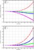 |
Fig. 1 The difference between the measured galaxy ellipticity estimates and their true, sheared ellipticities is shown as a function of the true ellipticity, for different measurement methods as indicated by the symbols. The ideal case of a measurement obtaining the true ellipticity precisely corresponds to the horizontal zero line. Top panel: ground-based observations with a wide point-spread function. Bottom panel: space-borne observations with a point-spread function of negligible width. |
The shear correlation function at a fixed scale is the average of the product of measured galaxy ellipticities at some angular separation. Therefore, what is relevant for our purposes here is the ellipticity rather than the shear calibration. In other terms, if one used the shear calibration derived from an experiment like the Shear TEsting Programme (STEP, Heymans et al. 2006) and used that to calibrate the galaxy ellipticities entering into the measurement of a correlation function, one would suffer from the bias in the cosmological parameters we are about to show here.
The ellipticity estimate is a
superposition of the intrinsic galaxy ellipticity and the applied cosmic shear. Since we
simulate the galaxy images with ellipticity χs and apply a known
reduced shear g, the true ellipticity is known to us. We compare this true
ellipticity to the measured ellipticity estimate obtained after PSF convolution by applying
the four named variants of KSB. The results are illustrated in Fig. 1 for two different choices of the PSF, where the difference between the
measured and the true ellipticities is plotted against the true ellipticity. Notice that,
even though the ellipticities in Fig. 1 appear quite
large,  , the
cosmic shear applied is |g| ≤ 0.1. By far the largest contribution to
is
due to the assumed intrinsic source ellipticity.
, the
cosmic shear applied is |g| ≤ 0.1. By far the largest contribution to
is
due to the assumed intrinsic source ellipticity.
The results shown in the two panels of Fig. 1 are based on a narrow PSF (bottom) mimicking a space-borne observation, and a wide PSF (top) that could be typical for a ground-based observation. Both PSFs are fully characterised by their Moffat exponent β and their FWHM. For the narrow PSF, (β,FWHM) = (2,0.5 Re); for the wide PSF, (β,FWHM) = (5,5 Re), where Re is the scale radius of the Sérsic profile assumed for the galaxy images. The ideal relation would follow the horizontal zero line. These figures illustrate three main points. First, the measured ellipticity estimate falls below or above the true ellipticity, depending on the method used for the interpretation of observed ellipticities. Second, the relations between measured ellipticity estimate and the true ellipticity are non-linear, which will turn into our main issue for this paper. Third, the deviation of the ellipticity estimate from the true shear, even its sign, depend on the width of the PSF. While KSB-3, for example, performs almost perfectly for a narrow PSF, it underestimates the true ellipticity if the PSF is wide. The origin of these trends has been identified in Viola et al. (2011). Here, we work out the consequences for the cosmological-parameter determinations from such measurements.
3. Biases on cosmological parameters
Given the non-linear relations between the ellipticity estimate and the true ellipticity, we now consider the following situation. Suppose a cosmic-shear observation is being carried out, surface-brightness moments are measured and converted to ellipticity estimates following one of the KSB variants described above, the shear correlation function is measured and cosmological parameters (essentially the matter density Ωm0 and the normalisation parameter σ8). Suppose further that the ellipticity estimate is in fact calibrated in the analysis process, e.g. by means of synthetic data, however assuming a linear rather than the underlying, non-linear relationship between the ellipticity estimate and the true ellipticity. In other words, the calibration is supposed to be carried out assuming that the response of the measurement to the shear is independent of the shear itself, rather than depending on it. Given such a procedure, which can perhaps be considered close to the common practice of identifying additive and multiplicative shear biases (Heymans et al. 2006), how biased would the cosmological parameters be, if at all?
To answer this question, the following steps need to be carried out:
First, we fix a reference cosmological model and compute the shear correlation function for
it. To be specific, we choose the correlation function
ξ+(θ), which is given by 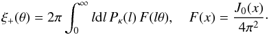 (8)The power spectrum
Pκ(l) of the convergence is
the usual weighted projection of the dark-matter fluctuation power spectrum
Pδ(k) in Limber’s
approximation. In a spatially-flat universe for sources at a fixed redshift,
(8)The power spectrum
Pκ(l) of the convergence is
the usual weighted projection of the dark-matter fluctuation power spectrum
Pδ(k) in Limber’s
approximation. In a spatially-flat universe for sources at a fixed redshift, 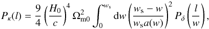 (9)where
w and ws are the comoving angular-diameter
distances to the lensing matter fluctuation and to the sources, respectively (see, e.g.,
Bartelmann 2010; Bartelmann & Schneider 2001, for a derivation).
(9)where
w and ws are the comoving angular-diameter
distances to the lensing matter fluctuation and to the sources, respectively (see, e.g.,
Bartelmann 2010; Bartelmann & Schneider 2001, for a derivation).
Second, we choose hypothetical survey parameters, define bins { θi } for the measurement of the correlation function and compute the covariance matrix Cij for the correlation function ξ+ between these bins. Doing so, we follow the procedure developed by Joachimi et al. (2008). This allows the computation of two important ingredients. First, we can choose the bins such that the signal-to-noise ratio is approximately the same in each bin. Second, we can calculate the expected uncertainties of the measured correlation function including their mutual correlation between bins. The latter step is conveniently achieved by rotating the bin vector into the principal-axis frame of the covariance matrix, drawing independent Gaussian random numbers with the appropriate variance, and inverting the rotation.
Next, we fit the calibration relations shown in Fig. 1
with a realistic quadratic dependence  (10)as well
as with an assumed linear dependence
(10)as well
as with an assumed linear dependence  (11)The correlation functions
of the shear estimate and the true shear are then related by
(11)The correlation functions
of the shear estimate and the true shear are then related by  (12)and must
be corrected accordingly by an offset and an amplitude to arrive at
ξ+. The offsets are
(12)and must
be corrected accordingly by an offset and an amplitude to arrive at
ξ+. The offsets are 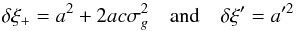 (13)for
the quadratic and linear relations, while the amplitudes are b2
and b′2, respectively. We shall assume in the following that the
offset can be faithfully corrected in any survey by demanding that the correlation function
approach zero at large angles. However, the correction of the amplitude remains. Our main
issue for the following discussion is that the amplitude b′2
derived from the assumed linear calibration relation differs from the amplitude
b2 expected from the realistic, quadratic calibration
relation. We thus assume that the measured shear correlation is corrected by
b′−2 while it should be corrected by
b-2. That is, we erroneously infer the correlation function
(13)for
the quadratic and linear relations, while the amplitudes are b2
and b′2, respectively. We shall assume in the following that the
offset can be faithfully corrected in any survey by demanding that the correlation function
approach zero at large angles. However, the correction of the amplitude remains. Our main
issue for the following discussion is that the amplitude b′2
derived from the assumed linear calibration relation differs from the amplitude
b2 expected from the realistic, quadratic calibration
relation. We thus assume that the measured shear correlation is corrected by
b′−2 while it should be corrected by
b-2. That is, we erroneously infer the correlation function
 (14)instead
of ξ+, which is then compared to theory and gives rise to a
bias in the cosmological parameters.
(14)instead
of ξ+, which is then compared to theory and gives rise to a
bias in the cosmological parameters.
The fit parameters b, c and b′ found for the four different variants of the KSB method are listed in Table 1. Due to the assumed offset correction, the parameters a and a′ are irrelevant.
Our third and final step is thus quite simple: we take the simulated correlation function
including its modelled uncertainty and error bars, multiply it by the factor
b2/b′2, and
then fit theoretical correlation functions to them minimising the
χ2 function
![Mathematical equation: \begin{equation} \chi^2 = \left[ \xi_{+, i}'-\xi_+(\theta_i, p)\right]C_{ij}^{-1}\left[\xi_{+, j}'-\xi_+(\theta_j, p) \right], \label{eq:16} \end{equation}](/articles/aa/full_html/2012/11/aa16983-11/aa16983-11-eq63.png) (15)where p
symbolically abbreviates all parameters entering the calculation of the theoretically
expected correlation function ξ+.
(15)where p
symbolically abbreviates all parameters entering the calculation of the theoretically
expected correlation function ξ+.
The χ2 contours following from this procedure are shown for three variants of KSB in Fig. 2.
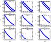 |
Fig. 2 Likelihood contours are shown in the Ωm0-σ8 plane for: a CFHT-like survey in the top row and a wide survey in the middle and bottom rows; three variants of the KSB method, i.e. KSB-tr in the left, KSB-1 in the middle and KSB-3 in the right columns; a wide PSF in the top and middle rows and a narrow PSF in the bottom row. The figure shows that cosmological parameters tend to be biased high for wide and low for narrow PSFs, and that the magnitude of the bias depends on the variant of KSB chosen. |
4. Results and conclusion
The χ2 contours shown in these figures were calculated assuming two different types of survey, whose parameters control the covariance matrices Cij. The assumed survey parameters are listed in Table 2. The cosmological parameters are set to Ωm0 = 0.3, ΩΛ0 = 1−Ωm0, h = 0.7 and σ8 = 0.8 in both cases.
Assumed parameters for a CFHT-like and a wider weak-lensing survey.
We leave out the original version of KSB because most of its likelihood contours fall off the parameter region shown. This is because the calibration relation of the original KSB method has the largest non-linear contribution and thus produces the strongest bias. The main pieces of information evident from Fig. 2 are:
-
The wide survey (results shown in the lower two rows) narrows the contours compared to the CFHT-like survey, but does otherwise not affect the results.
-
For a wide PSF (results shown in the upper two rows), cosmological parameters inferred from the likelihood contours are biased high for the first- and third-order KSB variants (second and third row), while KSB-tr is almost perfectly unbiased even with the narrow contours of the wide survey. The bias is mild for KSB-1 and substantial for KSB-3. This reflects the shape of the calibration curves for the wide PSF as shown in the lower panel of Fig. 1. Since they are convex from above, a linear fit to them overestimates the shear and thus leads to an overestimate of the shear correlation amplitude.
-
For a narrow PSF (results shown in the lower row), the inferred cosmological parameters are biased low for KSB-tr and KSB-1, while they are almost unbiased for KSB-3. The explanation is similar as above, since now the calibration relations are convex from below, causing linear fits to underestimate the shear.
-
The fact that the response of the KSB method to the ellipticity depends on the ellipticity itself, leading to a non-linear calibration relation between the ellipticity estimate and the true ellipticity, gives rise to possibly substantial biases in cosmological-parameter estimates if a linear calibration relation is assumed.
-
The success of different variants of KSB depends on the width of the PSF, and thus on the circumstances of the survey. Narrow PSFs tend to cause overestimates which wide PSFs tend to cause underestimates.
-
Good results of one variant of KSB, such as KSB-tr for a wide PSF, do not allow one to conclude that this variant performs well under all circumstances.
-
The calibration bias demonstrated here is not inevitable, but arises from an assumed linear calibration relation. Our results argue for allowing calibration relations, which are at least quadratic.
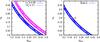 |
Fig. 3 Comparison between the likelihood contours in the Ωm0-σ8 plane for two different types of bias. Left panel: no bias due to ellipticity calibration was assumed, but the source-redshift estimate was assumed to be off by Δzs = 0.05 and Δzs = −0.1, as indicated by the line type. The right panel is the same as the bottom-left panel in Fig. 2. A wide survey was assumed for both panels. The comparison shows that, for a wide survey with narrow PSF, the calibration bias can be comparable or larger than a realistic bias due to an erroneous source redshift. |
Compared to other potential biases in cosmological constraints from weak lensing, the calibration bias can be substantial. Figure 3 opposes likelihood contours in the Ωm0-σ8 plane for a wide survey, in the left panel without calibration bias in the ellipticity measurement but a bias in the source redshift, and in the right panel without redshift bias but with the calibration bias of the KSB-tr method. The comparison shows that the calibration bias can be as large as a bias to a source redshift estimate off by Δz ≈ −0.1.
Our main concern is not to criticise KSB or its variants, but to emphasise that KSB, in all of its variants, causes a non-linear relation between ellipticity estimates and the true ellipticity. For some variants, the non-linearity is stronger or weaker, depending on circumstances, and some variants are mathematically more consistent than others. Our main conclusion, instead, fits into one statement: Without taking account of its non-linear calibration relation, KSB tends to give biased results. A new method avoiding these problems, called DEIMOS, was proposed by Melchior et al. (2011).
Other methods to estimate the ellipticity may show similar behaviour. Users concerned with highly accurate shear
estimation should therefore investigate whether the method employed exhibits an ellipticity-dependent bias, and if so, whether the shape and parameters of the inferred calibration relation are applicable to the survey at hand. This requires that the simulation, from which the calibration is to be inferred, mimics the actual survey data sufficiently closely, in particular with respect to PSF width and the distributions of galaxy size and ellipticity as well as their variations with redshift and signal-to-noise ratio.
Acknowledgments
We gratefully acknowledge helpul and improving comments by Catherine Heymans and Thomas Erben, and substantial clarification by an anonymous referee. This work was supported in part by the Schwerpunktprogramm 1177 and the Transregio-SFB 33 of the Deutsche Forschungsgemeinschaft, the European RTN “DUEL” and the Heidelberg Graduate School of Fundamental Physics. P.M. was supported by the US Department of Energy under Contract No. DE-FG02-91ER40690.
References
- Bartelmann, M. 2010, Class. Quant. Grav., 27, 233001 [CrossRef] [Google Scholar]
- Bartelmann, M., & Schneider, P. 2001, Phys. Rep., 340, 291 [NASA ADS] [CrossRef] [Google Scholar]
- Bernstein, G. M., & Jarvis, M. 2002, AJ, 123, 583 [NASA ADS] [CrossRef] [Google Scholar]
- Bridle, S., Balan, S. T., Bethge, M., et al. 2010, MNRAS, 405, 2044 [NASA ADS] [Google Scholar]
- Heymans, C., Van Waerbeke, L., Bacon, D., et al. 2006, MNRAS, 368, 1323 [NASA ADS] [CrossRef] [Google Scholar]
- Hoekstra, H. 2007, MNRAS, 379, 317 [NASA ADS] [CrossRef] [Google Scholar]
- Joachimi, B., Schneider, P., & Eifler, T. 2008, A&A, 477, 43 [NASA ADS] [CrossRef] [EDP Sciences] [Google Scholar]
- Kaiser, N., Squires, G., & Broadhurst, T. 1995, ApJ, 449, 460 [NASA ADS] [CrossRef] [Google Scholar]
- Kuijken, K. 1999, A&A, 352, 355 [NASA ADS] [Google Scholar]
- Melchior, P., Viola, M., Schäfer, B. M., & Bartelmann, M. 2011, MNRAS, 412, 1552 [NASA ADS] [CrossRef] [Google Scholar]
- Miller, L., Kitching, T. D., Heymans, C., Heavens, A. F., & van Waerbeke, L. 2007, MNRAS, 382, 315 [NASA ADS] [CrossRef] [Google Scholar]
- Schrabback, T., Hartlap, J., Joachimi, B., et al. 2010, A&A, 516, A63 [NASA ADS] [CrossRef] [EDP Sciences] [Google Scholar]
- Viola, M., Melchior, P., & Bartelmann, M. 2011, MNRAS, 410, 2156 [NASA ADS] [CrossRef] [Google Scholar]
- Voigt, L. M., & Bridle, S. L. 2010, MNRAS, 404, 458 [NASA ADS] [Google Scholar]
All Tables
All Figures
|
Fig. 1 The difference between the measured galaxy ellipticity estimates and their true, sheared ellipticities is shown as a function of the true ellipticity, for different measurement methods as indicated by the symbols. The ideal case of a measurement obtaining the true ellipticity precisely corresponds to the horizontal zero line. Top panel: ground-based observations with a wide point-spread function. Bottom panel: space-borne observations with a point-spread function of negligible width. |
| In the text | |
|
Fig. 2 Likelihood contours are shown in the Ωm0-σ8 plane for: a CFHT-like survey in the top row and a wide survey in the middle and bottom rows; three variants of the KSB method, i.e. KSB-tr in the left, KSB-1 in the middle and KSB-3 in the right columns; a wide PSF in the top and middle rows and a narrow PSF in the bottom row. The figure shows that cosmological parameters tend to be biased high for wide and low for narrow PSFs, and that the magnitude of the bias depends on the variant of KSB chosen. |
| In the text | |
|
Fig. 3 Comparison between the likelihood contours in the Ωm0-σ8 plane for two different types of bias. Left panel: no bias due to ellipticity calibration was assumed, but the source-redshift estimate was assumed to be off by Δzs = 0.05 and Δzs = −0.1, as indicated by the line type. The right panel is the same as the bottom-left panel in Fig. 2. A wide survey was assumed for both panels. The comparison shows that, for a wide survey with narrow PSF, the calibration bias can be comparable or larger than a realistic bias due to an erroneous source redshift. |
| In the text | |
Current usage metrics show cumulative count of Article Views (full-text article views including HTML views, PDF and ePub downloads, according to the available data) and Abstracts Views on Vision4Press platform.
Data correspond to usage on the plateform after 2015. The current usage metrics is available 48-96 hours after online publication and is updated daily on week days.
Initial download of the metrics may take a while.