© ESO, 2012

1. Introduction

Supernovae (SNe) Ia are extensively used for deriving extragalactic distances, because in the last two decades they turned out to be precise and reliable distance indicators (see e.g. Matheson et al. 2012, and references therein). Although they are not standard candles in the optical (contrary to the widespread statements that they are, which appear frequently even in the most recent papers), their light curve (LC) shape correlates with their peak absolute magnitude, making them standardizable (or calibratable) objects. The main advantage of applying SNe Ia for distance measurement is that the method is essentially photometric and does not need spectroscopy, save for typing the SN as a Ia.

The LC shape is connected with the peak brightness via the “Phillips-relation” (Phillips 1993), which states that SNe Ia that decline more slowly after maximum have intrinsically brighter peak magnitude, and vice versa. Although there are attempts to explain this phenomenon based on theoretical grounds (Hoeflich et al. 1996; Pinto & Eastman 2001; Kasen & Woosley 2007), this “peak magnitude – LC properties” relation is still mostly empirical at present. Therefore, the whole procedure of getting distances from the photometry of SNe Ia relies on empirical calibrations of the SNe Ia peak brightnesses, which need accurate, independent distances as well as other details like reddening and intrinsic color for the calibrating objects. This is the major source of the relatively small, but still existing random and systematic errors that limit the precision and accuracy of the derived distances (see e.g. Mandel et al. 2011, for further discussion and references).

SN 2011fe (aka PTF11kly, Nugent et al. 2011) is an excellent object in this respect, because this bright (m_peak ~ 10 mag), nearby (D ~ 6.5 Mpc) SN Ia was discovered hours after explosion (Nugent et al. 2011; Bloom et al. 2012) and suffered from very little interstellar reddening (A_V ~ 0.04 mag, Nugent et al. 2011; Patat et al. 2012). The high apparent brightness allowed us to obtain accurate, high signal-to-noise photometry, while the very low redshift (z = 0.000804, de Vaucouleurs et al. 1991) of its host galaxy, M101 (NGC 5457), eliminates the necessity of K-corrections for the photometry that otherwise would be a major source of systematic errors plaguing the distance determination (Hsiao et al. 2007; Hsiao 2009). The low interstellar reddening is also a very fortunate circumstance, because all complications regarding the handling of the effect of interstellar dust (galactic vs. non-standard reddening, disentangling reddening and intrinsic color variation, etc.) are expected to be minimal. Also, the host galaxy, M101, has many recently published distance estimates by various methods including Cepheids (Freedman et al. 2001; Shappee & Stanek 2011). Therefore, SN 2011fe is an ideal object to test the current state-of-the-art of the SN Ia LC fitters.

In this paper we present new, homogeneous, calibrated (BVRI) photometry for SN 2011fe obtained with a single telescope/detector combination (Sect. 2). We apply the two most widely accepted and trusted, independently calibrated, public LC fitters for SNe Ia, MLCS2k2 (Jha et al. 2007) and SALT2 (Guy et al. 2007) to derive photometric distances to M101 from our data (Sect. 3). The results are compared with other M101 distance estimates in Sect. 4. Section 5 summarizes our results.

2. Observations

2.1. Photometry of SN 2011fe

We have obtained multi-color ground-based photometric observations for SN 2011fe from the Piszkéstető Mountain Station of the Konkoly Observatory, Hungary. We used the 60/90 cm Schmidt-telescope with the attached 4096 × 4096 CCD (FoV 70 × 70 arcmin², equipped with Bessel BVRI filters). In Table 1 the data for the first 41 nights are presented. Note that we use JD instead of MJD throughout this paper.

The magnitudes were obtained by applying aperture photometry using the daophot/phot task in IRAF¹. Because the background level around the SN position is relatively low and uniform (see Fig. 1), neither PSF-photometry, nor image subtraction were necessary to get reliable light curves for SN 2011fe.

Transformation to the standard system was computed by using color terms expressed in the following forms for the V magnitude and the color indices: 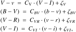$\begin{array}{ccc}& & \mathit{V}\mathrm{-}\mathit{v} \mathrm{=} {\mathit{C}}_{\mathrm{V}}\mathrm{·}\mathrm{(}\mathit{V}\mathrm{-}\mathit{I}\mathrm{)}\mathrm{+}{\mathit{\zeta }}_{\mathit{V}}\\ & & \mathrm{(}\mathit{B}\mathrm{-}\mathit{V}\mathrm{)} \mathrm{=} {\mathit{C}}_{\mathit{BV}}\mathrm{·}\mathrm{(}\mathit{b}\mathrm{-}\mathit{v}\mathrm{)}\mathrm{+}{\mathit{\zeta }}_{\mathit{BV}}\\ & & \mathrm{(}\mathit{V}\mathrm{-}\mathit{R}\mathrm{)} \mathrm{=} {\mathit{C}}_{\mathit{VR}}\mathrm{·}\mathrm{(}\mathit{v}\mathrm{-}\mathit{r}\mathrm{)}\mathrm{+}{\mathit{\zeta }}_{\mathit{VR}}\\ & & \mathrm{(}\mathit{V}\mathrm{-}\mathit{I}\mathrm{)} \mathrm{=} {\mathit{C}}_{\mathit{VI}}\mathrm{·}\mathrm{(}\mathit{v}\mathrm{-}\mathit{i}\mathrm{)}\mathrm{+}{\mathit{\zeta }}_{\mathit{VI}}\mathit{,}\end{array}$(1)where lowercase symbols denote the instrumental magnitudes, while uppercase letters mean standard magnitudes. The color terms were determined by measuring Landolt standard stars in the field of PG2213 observed during photometric conditions: C_V = −0.019, C_BV = 1.218, C_VR = 1.035, C_VI = 0.959. These values were kept fixed while computing the standard magnitudes for the whole dataset.

Zero-points (ζ_X) for each night were measured using local tertiary standard stars (Table 2). These local comparison stars were tied to the Landolt standards during the photometric calibration.

Additional unfiltered photometry has been carried out at the Baja Observatory of Bács-Kiskun County, Baja, Hungary with the 50 cm automated BART-telescope equipped with a 4096 × 4096 back-illuminated Apogee Ultra CCD (FoV 40 × 40 arcmin², the frames were taken with 2 × 2 binning). During the course of the Baja-Szeged-Supernova-Survey (BASSUS) the field of M101 was imaged with BART on 2011-08-22.9 UT,  ~2 days before discovery. No object was detected at the position of SN 2011fe brighter than  ~18.5 R-band magnitude. After discovery, unfiltered photometric observations were taken on 25 nights between Aug. 26 and Nov. 6, 2011 (Table 3). These data were scaled to the properly calibrated R-band observations from Konkoly Observatory and used only in constraining the the moment of explosion and the time of maximum light.

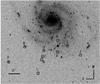Fig. 1 The field around SN 2011fe (marked by two line segments) with the local comparison stars encircled.

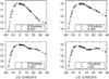Fig. 2 Comparison of LCs from Konkoly and RIT Observatories.

Calibrated photometry for SN 2011fe have also been collected from recent literature. Richmond & Smith (2012) presented BVRI photometry obtained at the Rochester Institute of Technology (RIT) Observatory, and at the Michigan State University Campus Observatory. A comparison between the Konkoly and RIT data are plotted in Fig. 2 (restricted to within 40 days around peak for better visibility) illustrating the excellent agreement between these independent datasets.

2.2. A UV-NIR spectrum of SN 2011fe

SN 2011fe was intensively followed up spectroscopically, and the spectroscopic evolution is discussed in detail in Parrent et al. (2012) and Smith et al. (2011). Expanding on that work is beyond the scope of this paper. Instead, we show only a single pre-maximum spectrum of SN 2011fe (Fig. 3) extending from the ultraviolet (UV) to the near infrared (NIR).

The spectrum plotted in Fig. 3 is a result of combining three datasets, obtained with different instruments. The optical data were obtained with the HET Marcario Low Resolution Spectrograph (LRS, spectral coverage 4200–10 200 Å, resolving power λ/Δλ ~ 600) at the McDonald Observatory, Texas, on Aug. 27, 2011. These data were reduced with standard IRAF routines. The UV part was taken by Swift/UVOT as a UGRISM observation on Aug. 28, 2011 (see Brown et al. 2012). The reduction was done with the routine uvotimgrism in HEASoft. The low (R ≈ 200) and medium (R ≈ 1200) resolution NIR spectra were obtained on August 26.3 UT with the 3.0 m telescope at the NASA Infrared Telescope Facility (IRTF) using the SpeX medium-resolution spectrograph (Rayner et al. 2003). The IRTF data were reduced using a package of IDL routines specifically designed for the reduction of SpeX data (Spextool v. 3.4, Cushing et al. 2004).

Figure 3 illustrates the unprecedented quality of data available for SN 2011fe, the analysis of which will be the topic of subsequent papers (e.g. a sequence of NIR spectra will be studied by Hsiao et al., in prep.). A similar extended spectrum for the Type Ia SN 2011iv has been recently published by Foley et al. (2012b). The SN 2011fe spectrum presented here is only the second such high-quality UVOIR spectrum for a Type Ia. These kind of data may be especially useful for theoretical modeling.

Comparison with spectra of other SNe (Cenko et al. 2011) revealed that SN 2011fe is a textbook-example of Branch-normal SNe Ia. The spectroscopic evidence that SN 2011fe is a “normal” (i.e. not peculiar) SN Ia strengthens the applicability of the LC fitting techniques (see above) that were calibrated for such SNe.

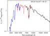Fig. 3 UV-NIR spectrum of SN 2011fe. Note that scales on both axes are logarithmic.

3. Analysis

This section contains a brief review of the LC fitting methods for SNe Ia. Their application to the observed data of SN 2011fe are then presented.

3.1. SN Ia light curve fitters

The empirical correlation between the LC shape and peak brightness of SNe Ia was first revealed by Phillips (1993), after the initial suggestion made by Pskovskii (1977). According to the Phillips-relation, SNe Ia that decline more slowly after maximum are intrinsically brighter than the more rapidly declining ones. Phillips (1993) introduced the Δm₁₅(B) parameter for measuring the decline rate: it gives the decrease of the SN brightness from the peak magnitude at 15 days after maximum in the B-band.

This concept was further examined and extended to other photometric bands by Riess et al. (1996), introducing the “Multi-Color Light Curve Shape” (MLCS) method. They defined a new parameter, Δ, for measuring the peak brightness as a function of the LC shape. Originally MLCS was calibrated for the Johnson-Cousins BVRI bands, and the LC in each band was described as a linear combination of two empirical (tabulated) curves and the parameter Δ. These curves were calibrated (“trained”) using 9 nearby, well-observed SNe Ia that had independent distances, mostly from the Tully-Fisher method. In Riess et al. (1998) MLCS was reformulated, expressing the LCs as a quadratic function of Δ and including the U-band (but see e.g. Kessler et al. 2009, for discussion on the utility of the U-band data).

In this paper we applied the latest version, MLCS2k2 (Jha et al. 2007), which further improved the calibration by applying a sample of 133 SNe Ia for training and also included a new parametrization for taking into account the effect of interstellar reddening. In this version the observed LC of a SN Ia can be expressed as $\begin{array}{ccc}{\mathit{m}}_{\mathit{x}}\mathrm{(}\mathit{t}\mathrm{-}{\mathit{t}}_{\mathrm{0}}\mathrm{)} \mathrm{=} {\mathit{M}}_{\mathit{x}}^{\mathrm{0}}\mathrm{(}\mathit{t}\mathrm{-}{\mathit{t}}_{\mathrm{0}}\mathrm{)}\mathrm{+}{\mathit{\mu }}_{\mathrm{0}}\mathrm{+}{\mathit{\zeta }}_{\mathit{x}}\left({\mathit{\alpha }}_{\mathit{x}}\mathrm{+}\frac{{\mathit{\beta }}_{\mathit{x}}}{{\mathit{R}}_{\mathrm{V}}}\right){\mathit{A}}_{\mathrm{V}}^{\mathrm{0}}& & \\ \mathrm{+}{\mathit{P}}_{\mathit{x}}\mathrm{(}\mathit{t}\mathrm{-}{\mathit{t}}_{\mathrm{0}}\mathrm{)}\mathrm{·}\mathrm{\Delta }\mathrm{+}{\mathit{Q}}_{\mathit{x}}\mathrm{(}\mathit{t}\mathrm{-}{\mathit{t}}_{\mathrm{0}}\mathrm{)}\mathrm{·}{\mathrm{\Delta }}^{\mathrm{2}}\mathit{,}& & \end{array}$(2)where t − t₀ is the SN phase in days, t₀ is the moment of maximum light in the B-band, m_x is the observed magnitude in the x-band (x = B,V,R,I), ${\mathit{M}}_{\mathit{x}}^{\mathrm{0}}\mathrm{(}\mathit{t}\mathrm{-}{\mathit{t}}_{\mathrm{0}}\mathrm{)}$ is the fiducial Ia absolute LC in the same band, μ₀ is the true (reddening-free) SN distance modulus, ζ_x, α_x and β_x are functions describing the interstellar reddening, R_V and ${\mathit{A}}_{\mathrm{V}}^{\mathrm{0}}$ are the ratio of total-to-selective absorption and the V-band extinction at maximum light, respectively, Δ is the main LC parameter, and P_x and Q_x are tabulated functions of the SN phase (“LC-vectors”). Together with Δ, the functions ${\mathit{M}}_{\mathit{x}}^{\mathrm{0}}$, P_x and Q_x describe the shape of the LC of a particular SN. For these functions we have applied the latest calibration downloaded from the MLCS2k2 website². Note that Jha et al. (2007) tied the MLCS2k2 LC-vectors to SNe Ia in the Hubble-flow adopting H₀ = 65 km s^-1 Mpc^-1. Thus, if needed, the distances given by MLCS2k2 may be rescaled to other values of H₀ by ${\mathit{\mu }}_{\mathrm{0}}\mathrm{\left(}{\mathit{H}}_{\mathrm{0}}\mathrm{\right)} \mathrm{=} {\mathit{\mu }}_{\mathrm{0}}\mathrm{\left(}\mathrm{MLCS}\mathrm{\right)}\mathrm{-}\mathrm{5}{\log }_{\mathrm{10}}\mathrm{(}{\mathit{H}}_{\mathrm{0}}\mathit{/}\mathrm{65}\mathrm{)} \mathrm{mag}\mathit{.}$(3)Another independent LC fitter, SALT2, was developed by the SuperNova Legacy Survey team (Guy et al. 2007). SALT2 is different from MLCS2k2 because it models the whole spectral energy distribution (SED) of a SN Ia as ${\mathit{F}}_{\mathit{\lambda }}\mathrm{\left(}\mathit{p}\mathrm{\right)} \mathrm{=} {\mathit{x}}_{\mathrm{0}}\mathrm{·}\mathrm{\left[}{\mathit{M}}_{\mathrm{0}}\mathrm{\right(}\mathit{p,\lambda }\mathrm{)}\mathrm{+}{\mathit{x}}_{\mathrm{1}}{\mathit{M}}_{\mathrm{1}}\mathrm{(}\mathit{p,\lambda }\mathrm{\left)}\mathrm{\right]}\exp \mathrm{[}\mathit{c}\mathrm{·}\mathit{CL}\mathrm{(}\mathit{\lambda }\mathrm{\left)}\mathrm{\right]}\mathit{,}$(4)where p = t − t₀ is the time from B-maximum (the SN phase), F_λ is the phase-dependent rest-frame flux density, M₀(p,λ), M₁(p,λ) and CL(λ) are the SALT2 trained vectors. The free parameters x₀, x₁ and c are the normalization-, stretch- and color parameters, respectively. We applied version 2.2.2b of the code³, which was trained with the SNLS 3-year data (Guy et al. 2010, G10 hereafter).

Because SALT2 models the entire SED, the observed LCs made with a particular filter set must be derived by synthetic photometry. SALT2 performs this computation based on the information provided by the user on the magnitude system in which the input data were taken. Since our photometry is in the Johnson-Cousins system (see Sect. 2), we have selected the standard Vega-magnitude system given in the code.

3.2. Constraining the moment of explosion and B-band maximum

Fig. 4 Fitting for the moment of explosion (left panel) and the time of B-band maximum (right panel).

Although the LC fitters applied in this paper use the time of B-band maximum light as the zero point of the time, the moment of explosion is also a very important physical parameter for SNe Ia. This can be inferred from the pre-maximum photometry. In this section we repeat the analysis of Nugent et al. (2011) to estimate this parameter for SN 2011fe using more data and a better sampled early LC.

The pre-maximum LC of SNe Ia can be surprisingly well described by the constant temperature “fireball” model (e.g. Arnett 1982; Nugent et al. 2011; Foley et al. 2012a). In this simple model the adiabatic loss of the ejecta internal energy is just compensated by the energy input from the radioactive decay of the ⁵⁶Ni and ⁵⁶Co synthesized during the explosion. This results in a nearly constant effective temperature and a luminosity governed only by the change of the photospheric radius, which, assuming homologous expansion, can be approximated as R_ph ~ t, giving L ~ t². Although this simple picture does not capture all the details in the pre-maximum ejecta, it provides a surprisingly good fit to the observations (see also Riess et al. 1999; Hayden et al. 2010; Ganeshalingam et al. 2011).

We have applied the function of m = −2.5log ₁₀(k·(t − t_exp)²) to the observed pre-maximum R-band magnitudes in Tables 1 and 3, supplemented by similar data collected from Nugent et al. (2011) and Richmond & Smith (2012). The fit parameters were k and t_exp, where the latter was further constrained by the epochs of published non-detections (Nugent et al. 2011; Bloom et al. 2012, and Table 3). The left panel of Fig. 4 shows the excellent agreement between the observed data and the fit t² law. The fitting resulted in t_exp = JD 2 455 797.216 ± 0.010, in perfect agreement with the value JD 2 455 797.187 ± 0.014 reported by Nugent et al. (2011). Relaxing the t² constraint to tⁿ and optimizing n gave n = 2.050 ± 0.025 and t_exp = JD 2 455 797.182 ± 0.021, which do not differ significantly from the results assuming t². We conclude that the explosion of SN 2011fe occured at JD 2 455 797.20 ± 0.16 (2011-08-23 16:48 UT ± 12 min).

The B-band data from Table 1 and from Richmond & Smith (2012) are also used to constrain the moment of B-maximum. Fitting a 4th order polynomial to the magnitudes obtained between +9 and +30 days after explosion resulted in t_Bmax = JD 2 455 814.4 ± 0.6, which was used as input for the LC fitter codes (see below). Thus, the B-band maximum occured  ~17.2 days after explosion, very similar to the value derived by Foley et al. (2012a) for SN 2009ig (17.13 days), which was also discovered in less than a day after explosion. The average value for the majority of “normal” SNe Ia is  ~17.4 ± 0.2 days (Hayden et al. 2010). This supports the conclusion from spectroscopy that SN 2011fe is a “normal” SN Ia.

3.3. Distance measurement

We have applied both MLCS2k2 and SALT2 to the observed BVRI data of SN 2011fe shown in Sect. 2.1. Before fitting, all data have been corrected for Milky Way reddening adopting A_V = 0.028 mag and E(B − V) = 0.009 mag (Schlegel et al. 1998). Note that these values are consistent with the recent recalibration of Milky Way reddening by Schlafly & Finkbeiner (2011).

Because of the low redshift of the host galaxy (z = 0.000804, see Sect. 1), K-corrections for transforming the observed magnitudes to rest-frame bandpasses are negligible, thus, they were ignored. We have not included U-band LC data (Brown et al. 2012) in either fitting, thus avoiding the persistent systematic uncertainties in modeling SNe Ia U-band data (e.g. Kessler et al. 2009).

Note that the absolute magnitudes of SNe Ia LCs were calibrated to different peak magnitudes in the two independent LC-fitters. MLCS2k2 was tied to SNe Ia distances assuming H₀ = 65 km s^-1 Mpc^-1 (Jha et al. 2007), while the peak magnitude in SALT2 was fixed assuming H₀ = 70 km s^-1 Mpc^-1 (G10). To get rid of this discrepancy, we have transformed all distance moduli given below to H₀ = 73 km s^-1 Mpc^-1 using Eq. (3).

Since the MLCS2k2 templates are defined between −10 and  + 90 days around B-maximum, while the SALT2 templates extend from −20 to only  + 50 days, we performed the LC fitting not only for all observed data (listed in Table 1), but also for those obtained between −7 and  + 40 days around B-maximum (JD 2 455 808 < t < 2 455 855). This test was performed in order to reach maximum compatibility between the applications of the two methods, and reduce the systematics that might bias the fitting results.

3.3.1. MLCS2k2

The fitting of Eq. (2) was performed by using a simple, self-developed χ²-minimization code, which scans through the allowed parameter space with a given step and finds the lowest χ² within this range. The fit parameters were the moment of B-maximum (t₀), the V-band extinction A_V, the LC-parameter Δ and the distance modulus μ₀, with steps of δt₀ = 0.1, δA_V = 0.01, δΔ = 0.01 and δμ₀ = 0.01, respectively. At the expense of longer computation time, this approach maps the entire χ² hypersurface and finds the absolute minimum in the given parameter volume.

We have fixed the reddening-law parameter as R_V = 3.1 appropriate for Milky Way reddening, although several recent results suggest that some high-velocity SNe Ia can be better modeled with significantly lower R_V (Wang et al. 2009; Foley & Kasen 2011). Since SN 2011fe suffered from only minor reddening and most of it is due to Milky Way dust (see below), it is more appropriate to adopt the galactic reddening law. Nevertheless, because of the low reddening, the value of R_V has negligible effect on the final distance.

The best-fitting MLCS2k2 model LCs are plotted together with the data in Fig. 5 (we plot only the results of fitting the whole dataset, because the fit to the restricted data range gave very similar results). The final parameters are given in Table 4 for both the whole and the restricted data. The 1σ uncertainties were estimated from the contour of Δχ² = 1 corresponding to 68% confidence interval. Figure 6 shows the map of the the χ² hypersurface and the shape of the contours around the minimum for the two key parameters Δ and μ₀. It is seen that μ₀ is strongly correlated with Δ, which is the major source of the relatively large uncertainty δμ = 0.07 mag, despite the very good fitting quality.

As seen in Table 4, there is no significant difference between the fit parameters for the two datasets. The host extinction (${\mathit{A}}_{\mathrm{V}}^{\mathrm{host}}$) is slightly less in the case of the restricted dataset, but that is compensated by the higher value of Δ (meaning fainter peak brightness), resulting in almost the same distance modulus. Thus, in the followings we adopt the parameters from fitting the full observed LC (left column in Table 4) as the final result from the particular LC-fitter, since those are based on the maximum available information.

Note that the best-fitting MLCS2k2 template LC corresponds to Δm₁₅(B) = 1.07 ± 0.06. Although Richmond & Smith (2012) gives 1.21 ± 0.03 for this parameter, this is probably a misprint since we measured 1.12 ± 0.05 from their published data, similar to the value of 1.10 ± 0.05 given by Tammann & Reindl (2011). It seems that all these parameters are consistent with each other, as well as with the finding that SN 2011fe has a nearly perfect fiducial SN Ia LC.

3.3.2. SALT2

Fig. 5 Fitting of the MLCS2k2 LCs to all observed data of SN 2011fe. Solid curves represent the best-fitting templates, while dotted curves denote the template uncertainties given by the time-dependent variance of each template curve.

The SALT2 fitting was computed by running the code as described on the SALT2 website. The fit parameters provided by the code are: ${\mathit{m}}_{\mathit{B}}^{\mathit{\star }}$ (rest-frame B-magnitude at maximum), x₁ (stretch) and c (color). Note that SALT2 restricts the fitting to data obtained no later than  + 40 days after maximum.

Contrary to MLCS, the SALT2 model does not explicitly include the distance or the distance modulus, thus, it must be derived from the fitting parameters. We followed two slightly different procedures for this: the one presented by G10 and an independent realization given by Kessler et al. (2009, K09 hereafter). Starting from the fitting parameters ${\mathit{m}}_{\mathit{B}}^{\mathit{\star }}$, x₁ and c, the distance modulus μ₀ in the G10 calibration can be obtained as $\begin{array}{ccc}{\mathit{m}}_{\mathit{BB}}& \mathrm{=}& {\mathit{m}}_{\mathit{B}}^{\mathit{\star }}\mathrm{-}\mathrm{0.008}\mathrm{(}\mathrm{\hspace{0.17em}\pm \hspace{0.17em}}\mathrm{0.005}\mathrm{)}\mathrm{·}{\mathit{x}}_{\mathrm{1}}\mathrm{+}\mathrm{0.013}\mathrm{(}\mathrm{\hspace{0.17em}\pm \hspace{0.17em}}\mathrm{0.004}\mathrm{)}\\ \mathit{CC}& \mathrm{=}& \mathrm{0.997}\mathrm{(}\mathrm{\hspace{0.17em}\pm \hspace{0.17em}}\mathrm{0.097}\mathrm{)}\mathrm{·}\mathit{C}\mathrm{+}\mathrm{0.002}\mathrm{(}\mathrm{\hspace{0.17em}\pm \hspace{0.17em}}\mathrm{0.009}\mathrm{)}\mathrm{·}{\mathit{x}}_{\mathrm{1}}\mathrm{+}\mathrm{0.035}\mathrm{(}\mathrm{\hspace{0.17em}\pm \hspace{0.17em}}\mathrm{0.008}\mathrm{)}\\ \mathit{s}& \mathrm{=}& \mathrm{0.107}\mathrm{(}\mathrm{\hspace{0.17em}\pm \hspace{0.17em}}\mathrm{0.006}\mathrm{)}\mathrm{·}{\mathit{x}}_{\mathrm{1}}\mathrm{+}\mathrm{0.991}\mathrm{(}\mathrm{\hspace{0.17em}\pm \hspace{0.17em}}\mathrm{0.006}\mathrm{)}\\ {\mathit{\mu }}_{\mathrm{0}}& \mathrm{=}& {\mathit{m}}_{\mathit{BB}}\mathrm{-}{\mathit{M}}_{\mathit{B}}\mathrm{+}\mathit{a}\mathrm{·}\mathrm{(}\mathit{s}\mathrm{-}\mathrm{1}\mathrm{)}\mathrm{-}\mathit{b}\mathrm{·}\mathit{CC,}\end{array}$(5)where we have adopted M_B = −19.218 ± 0.032, a = 1.295 ± 0.112 and b = 3.181 ± 0.131 (G10).

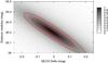Fig. 6 Map of the χ2 hypersurface around the minimum for MLCS2k2 fitting to all data. The contours correspond to 68, 90 and 95% confidence intervals (from inside to outside), respectively.

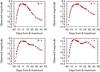Fig. 7 Fitting of SALT2 LCs to the observed data of SN 2011fe.

The K09 calibration applies a simpler formula: ${\mathit{\mu }}_{\mathrm{0}} \mathrm{=} {\mathit{m}}_{\mathit{B}}^{\mathit{\star }}\mathrm{-}{\mathit{M}}_{\mathrm{0}}\mathrm{+}\mathit{\alpha }\mathrm{·}{\mathit{x}}_{\mathrm{1}}\mathrm{-}\mathit{\beta }\mathrm{·}\mathit{c,}$(6)where M₀ = −19.157 ± 0.025, α = 0.121 ± 0.027 and β = 2.63 ± 0.22 have been adopted from K09.

The uncertainties in the formulae above were taken into account by a Monte-Carlo technique: we calculated 10 000 different realizations of the above parameters by adding Gaussian random numbers having standard deviations equal to the uncertainties above to the mean values of all parameters and derived μ₀ from each randomized set of parameters applying Eqs. (5) and (6). Then the average and the standard deviation of the resulting sample of μ₀ values are adopted as the SALT2 estimate for the distance modulus and its uncertainty. Table 5 lists the best-fitting parameters and errors, again for both the whole and the restricted dataset. The final SALT2 distance modulus was obtained as an unweigthed average of the two values from the G10 and K09 calibrations.

4. Discussion

The application of MLCS2k2 and SALT2 LC-fitters for all observed data resulted in distance moduli of μ₀(MLCS2k2) = 29.21  ±  0.07 and μ₀(SALT2) = 29.05 ± 0.08, respectively. It is seen that there is a  ~2σ disagreement between these two values. Taking into account that these distance moduli were obtained by fitting the same, homogeneous, densely-sampled, high-quality photometric data of a nearby SN, and both codes provided excellent fitting quality, this Δμ₀ = 0.16 mag disagreement is rather discouraging. Note that the difference exists despite correcting the results from both codes to the same Hubble-constant, H₀ = 73 km s^-1 Mpc^-1 (see above).

Restricting the LC fitting only to data taken between −7 and  + 40 days around B-maximum (right column in Tables 4 and 5), the two distance moduli are both slightly higher and closer to one another: μ₀(MLCS2k2) = 29.23  ± 0.07 and μ₀(SALT2) = 29.10 ± 0.08, giving Δμ₀ = 0.13 mag. Since these parameters are generally within the errors of those from fitting the complete LC, the  ~2σ disagreement still persists.

A similar, even larger difference of μ₀(SALT2) − μ₀(MLCS2k2) =  ± 0.2 mag was found by K09 for the “Nearby SNe” sample of Jha et al. (2007), although deviations in both positive and negative directions have been revealed for individual SNe. Because the Nearby sample contains only a few very close, unreddened SNe like SN 2011fe, the source of the mild discrepancy found by K09 is ambiguous. The present results suggest that, because of the lack of issues due to reddening, K-correction, U-band anomaly or spectral peculiarities in the case of SN 2011fe (see Sect. 1), the >0.1 mag difference between the MLCS2k2 and SALT2 distance moduli is probably entirely due to a systematic offset between the different zero-point calibrations of the fiducial SN peak magnitude in the two methods.

In order to test this statement, we have compared the parameters in Tables 4 and 5. It is seen that for the whole dataset SALT2 estimates the B-maximum (t₀) as being 0.9 day later than the epoch provided by MLCS2k2. The result from the simple polynomial fitting (Sect. 3.2) is closer to the MLCS2k2 value, thus SALT2 might tend to overestimate this parameter. For the restricted data the final t₀ from both methods changed slightly, becoming more similar, but a difference of  ~0.5 day is still present.

In order to investigate whether the uncertainty of t₀ could be responsible for the systematic difference between the distance moduli, we have re-run the MLCS2k2 fitting for the restricted dataset by forcing t₀ equal to the SALT2 value of 2 455 815.395. This resulted in Δ = 0.054 mag and μ₀ = 29.205 mag with χ² = 0.3242 (${\mathit{A}}_{\mathrm{V}}^{\mathrm{host}}$ remained the same). The changes of the parameters are consistent with the shape of the χ² surface plotted in Fig. 6: if Δ is increased, then μ₀ decreases. This lower μ₀ is indeed closer to the SALT2 value, but a systematic difference of  ~0.1 mag still remains (i.e. the MLCS2k2 distance is still higher), while the quality of the fitting is clearly worse. Thus, while forcing t₀ to be equal to the SALT2 value may somewhat reduce the systematic difference between the two methods, not all of the systematics affecting the distance modulus can be explained by this parameter alone.

Distance measurements independent from these SN Ia LC-fitters may help in resolving the open issue of absolute magnitude and distance calibrations. Recently, Matheson et al. (2012) published distance estimates to SN 2011fe based on near-infrared (NIR) photometry. Because SNe Ia appear to be much better standard candles in the NIR than in optical bands, the usage of good-quality NIR photometry for this bright, nearby SN looks promising. Unfortunately, as Matheson et al. (2012) concluded, the present state-of-the-art of getting SNe Ia NIR distances also suffers from an unsolved zero-point calibration problem. This resulted in a wide range of NIR distance moduli for SN 2011fe spanning from 28.84 to 29.14 mag (corrected to H₀ = 73, as above) with a mean value of μ₀(NIR) = 29.0  ±  0.2 mag (Matheson et al. 2012). This is consistent with the SALT2 result above, but it also agrees marginally (at  ~1σ) with the MLCS2k2 distance modulus. The range of the NIR distance moduli from different calibrations, 0.31 mag (Matheson et al. 2012), is a factor of 2 larger than the uncertainties of the individual calibrations (~0.15 mag) of NIR peak magnitudes of SNe Ia. This may also be a warning sign that the distance measurement technique from NIR LCs of SNe Ia is far from being settled.

The situation is not much better if one considers the various distance estimates available for the host galaxy, M101. This is one of the closest, brightest, and most thoroughly studied galaxies for which Cepheid-based distances are available (see e.g. Matheson et al. 2012, and references therein). The most widely accepted distance modulus of M101 is 29.13 ± 0.11 mag from the Cepheid PL-relation by the HST Key Project (Freedman et al. 2001), which is just in the middle between the MLCS2k2 and SALT2 distance moduli above, being in 1σ agreement with both. More recently Shappee & Stanek (2011) obtained 29.04 ± 0.19 mag from an independent study of M101 Cepheids, which agrees better with the SALT2 estimate, although its larger errors makes the result also consistent with MLCS2k2. Shappee & Stanek (2011) adopted the maser distance of NGC 4258 as their distance anchor, which gives a lower distance modulus for the LMC by 0.09 mag than the value adopted by Freedman et al. (2001). This accounts for most of the difference between the two Cepheid-based results. Both of these Cepheid distances are slightly higher than the NIR-distance of Matheson et al. (2012), but considering the larger errors of the latter (0.2 mag), the three estimates are all more-or-less consistent with each other.

Non-Cepheid distance estimates to M101 span a  ~0.35 mag wide range, from 29.05 (from the Tip of the Red Giant Branch method, TRGB, Shappee & Stanek 2011) to 29.42 (based on Planetary Nebulae Luminosity Function, PNLF, Feldmeier et al. 1996), which does not help much in resolving the issue of the M101 distance (see Fig. 3 of Matheson et al. 2012).

5. Conclusions

The nearby, bright, weakly reddened Type Ia supernova 2011fe in M101 provides a unique opportunity to test both the precision and the accuracy of the extragalactic distances derived from SNe Ia LC fitters. In this paper we presented new, calibrated BVRI-photometry for SN 2011fe. The LCs were analyzed with publicly available LC-fitters MLCS2k2 and SALT2 to get the SN Ia-based distance to M101. There is a systematic offset of  ~0.15 mag between the MLCS2k2 and SALT2 distance moduli, the average of which also differs by  ~0.13 mag from the distance estimate by Matheson et al. (2012) from SN 2011fe NIR photometry. This systematic offset between the results of the two widely-used LC-fitters may be partly due to the different shape of the LC vectors near maximum, affecting the estimate of the moment of maximum light, but the majority of the offset is probably caused by systematic errors of the peak magnitudes from different photometric calibrations.

We conclude that the weighted average of the three distance moduli of SN 2011fe (using the inverse of the uncertainties as weights), μ₀(MLCS2k2), μ₀(SALT2) and μ₀(NIR) (Matheson et al. 2012), and the two Cepheid-based distance to M101 (Freedman et al. 2001; Shappee & Stanek 2011) provides the following distance modulus of M101: ${\mathit{\mu }}_{\mathrm{0}\mathit{,}\mathrm{M}\mathrm{101}} \mathrm{=} \mathrm{29.109}\mathrm{\hspace{0.17em}\pm \hspace{0.17em}}\mathrm{0.049} \mathrm{\left(}\mathrm{random}\mathrm{\right)} \mathrm{\hspace{0.17em}\pm \hspace{0.17em}} \mathrm{0.1} \mathrm{\left(}\mathrm{syst}\mathrm{\right)} \mathrm{mag}\mathit{,}$which corresponds to D_M101 = 6.6 ± 0.5 Mpc, taking into account both random and systematic uncertainties. Despite the exceptional quality of the measured LCs of SN 2011fe and the long history of efforts devoted to the calibration of LC-fitters for Ia SNe as well as the absolute distance to M101, the available techniques cannot predict the absolute distance to M101 with better than 0.5 Mpc (~8%) accuracy.

Acknowledgments

We are indebted to the referee, Peter Nugent, for his valuable comments and suggestions that helped us improving the paper. This project has been supported by Hungarian OTKA grant K76816, by NSF Grant AST 11-09881 (to J.C.W.), and by the European Union together with the European Social Fund through the TÁMOP 4.2.2/B-10/1-2010-0012 grant. G.H.M. and the CfA Supernova Program is supported by NSF Grant AST 09-07903. G.H.M. is a visiting Astronomer at the Infrared Telescope Facility, which is operated by the University of Hawaii under Cooperative Agreement No. NNX-08AE38A with the National Aeronautics and Space Administration, Science Mission Directorate, Planetary Astronomy Program. A.P. has been supported by the ESA grant PECS 98073 and by the János Bolyai Research Scholarship of the Hungarian Academy of Sciences. T.K. has been supported by OTKA Grant K81373. K.S., L.L.K. and K.V. acknowledge support from the “Lendület” Young Researchers’ Program of the Hungarian Academy of Sciences and the Hungarian OTKA Grants MB08C 81013, K83790 and K81421. J.C.W. is grateful for the hospitality of the Aspen Center for Physics supported by NSF PHY-1066293. Thanks are also due to the staff of McDonald and Konkoly Observatories for the prompt scheduling and helpful assistance during the time-critical ToO observations. The Hobby-Eberly Telescope (HET) is a joint project of the University of Texas at Austin, the Pennsylvania State University, Stanford University, Ludwig-Maximilians-Universitt Mnchen, and Georg-August-Universitt Gttingen. The HET is named in honor of its principal benefactors, William P. Hobby and Robert E. Eberly. The SIMBAD database at CDS, the NASA ADS and NED databases have been used to access data and references. The availability of these services is gratefully acknowledged.

References

All Tables

All Figures

	Fig. 1 The field around SN 2011fe (marked by two line segments) with the local comparison stars encircled.
In the text

	Fig. 2 Comparison of LCs from Konkoly and RIT Observatories.
In the text

	Fig. 3 UV-NIR spectrum of SN 2011fe. Note that scales on both axes are logarithmic.
In the text

	Fig. 4 Fitting for the moment of explosion (left panel) and the time of B-band maximum (right panel).
In the text

	Fig. 5 Fitting of the MLCS2k2 LCs to all observed data of SN 2011fe. Solid curves represent the best-fitting templates, while dotted curves denote the template uncertainties given by the time-dependent variance of each template curve.
In the text

	Fig. 6 Map of the χ2 hypersurface around the minimum for MLCS2k2 fitting to all data. The contours correspond to 68, 90 and 95% confidence intervals (from inside to outside), respectively.
In the text

	Fig. 7 Fitting of SALT2 LCs to the observed data of SN 2011fe.
In the text

References

- Arnett, W. D. 1982, ApJ, 253, 785 [NASA ADS] [CrossRef] [Google Scholar]
- Bloom, J. S., Kasen, D., Shen, Ken, J., et al. 2012, ApJ, 744, L17 [NASA ADS] [CrossRef] [Google Scholar]
- Brown, P. J., Dawson, K. S., de Pasquale, M., et al. 2012, ApJ, 753, 22 [NASA ADS] [CrossRef] [Google Scholar]
- Cenko, S. B., Thomas, R. C., Nugent, P. E., et al. 2011, The Astronomer’s Telegram, 3583, 1 [Google Scholar]
- Cushing, M. C., Vacca, W. D., & Rayner, J. T. 2004, PASP, 116, 362 [NASA ADS] [CrossRef] [Google Scholar]
- Feldmeier, J. J., Ciardullo, R., & Jacoby, G. H. 1996, ApJ, 461, L25 [NASA ADS] [CrossRef] [Google Scholar]
- Foley, R. J., & Kasen, D. 2011, ApJ, 729, 55 [NASA ADS] [CrossRef] [Google Scholar]
- Foley, R. J., Challis, P. J., Filippenko, A. V., et al. 2012a, ApJ, 744, 38 [NASA ADS] [CrossRef] [Google Scholar]
- Foley, R. J., Kromer, M., Howie Marion, G., et al. 2012b, ApJ, 753, L5 [Google Scholar]
- Freedman, W. L., Madore, B. F., Gibson, B. K., et al. 2001, ApJ, 553, 47 [NASA ADS] [CrossRef] [Google Scholar]
- Ganeshalingam, M., Li, W., & Filippenko, A. V. 2011, MNRAS, 416, 2607 [NASA ADS] [CrossRef] [Google Scholar]
- Guy, J., Astier, P., Baumont, S., et al. 2007, A&A, 466, 11 [NASA ADS] [CrossRef] [EDP Sciences] [Google Scholar]
- Guy, J., Sullivan, M., Conley, A., et al. 2010, A&A, 523, A7 [NASA ADS] [CrossRef] [EDP Sciences] [Google Scholar]
- Hayden, B. T., Garnavich, P. M., Kessler, R., et al. 2010, ApJ, 712, 350 [NASA ADS] [CrossRef] [Google Scholar]
- Hoeflich, P., Khokhlov, A., Wheeler, J. C., et al. 1996, ApJ, 472, L81 [NASA ADS] [CrossRef] [Google Scholar]
- Hsiao, Y. C. E. 2009, Ph.D. Thesis [Google Scholar]
- Hsiao, E. Y., Conley, A., Howell, D. A., et al. 2007, ApJ, 663, 1187 [NASA ADS] [CrossRef] [Google Scholar]
- Jha, S., Riess, A. G., & Kirshner, R. P. 2007, ApJ, 659, 122 [NASA ADS] [CrossRef] [Google Scholar]
- Kasen, D., & Woosley, S. E. 2007, ApJ, 656, 661 [NASA ADS] [CrossRef] [Google Scholar]
- Kessler, R., Becker, A. C., Cinabro, D., et al. 2009, ApJS, 185, 32 [NASA ADS] [CrossRef] [Google Scholar]
- Mandel, K. S, Narayan, G., & Kirshner, R. P. 2011, ApJ, 731, 120 [NASA ADS] [CrossRef] [Google Scholar]
- Matheson, T., Joyce, R. R., Allen, L. E., et al. 2012, ApJ, 754, 19 [NASA ADS] [CrossRef] [Google Scholar]
- Nugent, P. E., Sullivan, M., Cenko, S. B., et al. 2011, Nature, 480, 344 [NASA ADS] [CrossRef] [Google Scholar]
- Parrent, J. T., Howell, D. A., Friesen, B., et al. 2012, ApJ, 752, L26 [NASA ADS] [CrossRef] [Google Scholar]
- Patat, F., Cordiner, M. A., Cox, N. L. J., et al. 2012, A&A, accepted [arXiv:1112.0247] [Google Scholar]
- Phillips, M. M. 1993, ApJ, 413, L105 [NASA ADS] [CrossRef] [Google Scholar]
- Pinto, P. A., & Eastman, R. G. 2001, New A, 6, 307 [Google Scholar]
- Pskovskii, I. P. 1977, AZh, 54, 1188 [NASA ADS] [Google Scholar]
- Rayner, J. T., Toomey, D. W., Onaka, P. M., et al. 2003, PASP, 115, 362 [NASA ADS] [CrossRef] [Google Scholar]
- Richmond, M. W., & Smith, H. A. 2012, J. Am. Ass. Variable Star Obs., accepted [arXiv:1203.4013] [Google Scholar]
- Riess, A. G., Press, W. H., & Kirshner, R. P. 1996, ApJ, 473, 88 [NASA ADS] [CrossRef] [Google Scholar]
- Riess, A. G., Filippenko, A. V., Challis, P., et al. 1998, AJ, 116, 1009 [NASA ADS] [CrossRef] [Google Scholar]
- Riess, A. G., Filippenko, A. V., Li, W., et al. 1999, AJ, 118, 2675 [NASA ADS] [CrossRef] [Google Scholar]
- Schlafly, E. F., & Finkbeiner, D. P. 2011, ApJ, 737, 103 [NASA ADS] [CrossRef] [Google Scholar]
- Schlegel, D. J., Finkbeiner, D. P., & Davis, M. 1998, ApJ, 500, 525 [NASA ADS] [CrossRef] [Google Scholar]
- Shappee, B. J., Stanek, K. Z. 2011, ApJ, 733, 124 [NASA ADS] [CrossRef] [Google Scholar]
- Smith, P. S., Williams, G. G., Smith, N., et al. 2011, ApJ, submitted [arXiv:1111.6626] [Google Scholar]
- Tammann, G. A., & Reindl, B. 2011, ApJ, submitted [arXiv:1112.0439] [Google Scholar]
- de Vaucouleurs, G., de Vaucouleurs, A., Corwin, H. G., Jr., et al. 1991, Third Reference Catalogue of Bright Galaxies (New York: Springer) [Google Scholar]
- Wang, X., Filippenko, A. V., Ganeshalingam, M., et al. 2009, ApJ, 699, L139 [NASA ADS] [CrossRef] [Google Scholar]
All Tables
Unfiltered (scaled to R-band) photometry of SN 2011fe from the Baja Observatory, Hungary.