© ESO, 2012

1. Introduction

Magnetohydrodynamic (MHD) waves are recognized as an efficient tool in diagnostics of the solar corona as well as of solar flares, see e.g. Roberts (2000), Nakariakov (2003), and Macnamara & Roberts (2010, 2011). Waves and oscillations are observed by modern imaging and spectral instruments in the visible light, EUV, X-ray and radio bands, and some of them can be interpreted in terms of MHD plasma theory. The magnetically dominated solar plasma can support the propagation of various types of waves. These MHD waves and oscillations have been investigated and analyzed in many theoretical and numerical studies. Among various studied cases we can distinguish propagating (De Moortel et al. 2002), slow magnetoacoustic standing (Ofman & Wang 2002; Nakariakov et al. 2004; Selwa et al. 2005; Zaqarashvili et al. 2005; Jelínek & Karlický 2009, 2010), fast magnetoacoustic: kink (Nakariakov et al. 1999; Aschwanden et al. 2002; Wang & Solanki 2004; Andries et al. 2005; Pascoe et al. 2010) and sausage modes (Pascoe et al. 2007, 2009). These modes have been observed with highly sensitive instruments such as SUMER (SoHO) and TRACE, as well as by other recent solar missions, e.g., EIS/Hinode or EUVI/STEREO. Also, compressible MHD waves (Ofman et al. 1999); De Moortel et al. (2000) and flare-generated global kink oscillations of solar coronal loops (Schrijver et al. 2002) were discovered; for a comprehensive review, see Nakariakov & Verwichte (2005).

The impulsively generated MHD waves and oscillations can be excited by various processes in the solar corona. The impulsive flare process, which provides either single or multiple sources of disturbances, is the most probable one. The impulsively generated magnetoacoustic waves are trapped in regions of higher density, i.e. in regions with a lower Alfvén speed, which act as waveguides. The periodicity of propagating fast sausage waves results from the time evolution of an impulsively generated signal (see Roberts et al. 1983, 1984 and Murawski & Roberts 1994). These waves in a coronal waveguide have three distinct phases: (1) periodic phase (long-period spectral components are fastest and they arrive first at the detection point); (2) quasi-periodic phase (both long and short-period spectral components arrive and interact); (3) decay (or Airy) phase, where the signal passes the detection point (Roberts et al. 1984).

The wavelet analysis of impulsively generated (fast sausage) magnetoacoustic wave trains shows the typical tadpole shape with a narrow-spectrum tail preceding a broadband head. These tadpole signatures (wavelet tadpole) were first observed by the SECIS instrument in the 1999 solar-eclipse data (see Katsiyannis et al. 2003). Similarly, Mészárosová et al. (2009a,b) detected for the first time the tadpoles in the wavelet spectra in some radio sources, which has also been confirmed numerically, see e.g. Nakariakov et al. (2004, 2005).

Owing to their enhanced density, current-sheets are the structures that can guide the MHD waves. Karlický et al. (2011) found the wavelet tadpoles in sources of the narrowband dm-spikes. These authors concluded that these wavelet tadpoles indicate that the magnetoacoustic waves propagate in the global current-sheet (current layer) in the turbulent reconnection outflows. This paper served as a motivation of a more extended and detailed study of the magnetoacoustic (fast sausage) waves in the current-sheet, see Jelínek & Karlický (2012).

The present paper extends our previous model (Jelínek & Karlický 2012). We study an evolution of the propagating fast sausage magnetoacoustic waves in a vertical flare current-sheet under the influence of gravity, which makes our model more realistic. Then we compare it with the gravity-free case. Because these processes are important for a diagnostics of solar flares, we analyze the computed waves in the same way as those observed, i.e., using the wavelet analysis method.

The structure of the present paper is as follows. Section 2 describes our numerical models, governing equations, initial conditions, and perturbations. In Sect. 3, the numerical results, obtained by means of our computer models, are shown and discussed. Finally, Sect. 4 presents our conclusions.

2. Physical model

2.1. Governing equations

In our numerical model of the vertical flare current-sheet in the gravitationally stratified solar atmosphere, the plasma dynamics is described by the two-dimensional (2D) time-dependent ideal magnetohydrodynamic equations, see e.g. Priest (1982): 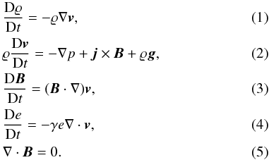$\begin{array}{ccc}& & \frac{\mathrm{D}\mathit{\varrho }}{\mathrm{D}\mathit{t}}\mathrm{=}\mathrm{-}\mathit{\varrho }\mathrm{\nabla }{v}\mathit{,}\\ & & \mathit{\varrho }\frac{\mathrm{D}{v}}{\mathrm{D}\mathit{t}}\mathrm{=}\mathrm{-}\mathrm{\nabla }\mathit{p}\mathrm{+}{j}\mathrm{\times }{B}\mathrm{+}\mathit{\varrho }{g}\mathit{,}\\ & & \frac{\mathrm{D}{B}}{\mathrm{D}\mathit{t}}\mathrm{=}\mathrm{(}{B}\mathrm{·}\mathrm{\nabla }\mathrm{)}{v}\mathit{,}\\ & & \frac{\mathrm{D}\mathit{e}}{\mathrm{D}\mathit{t}}\mathrm{=}\mathrm{-}\mathit{\gamma e}\mathrm{\nabla }\mathrm{·}{v}\mathit{,}\\ & & \mathrm{\nabla }\mathrm{·}{B}\mathrm{=}\mathrm{0.}\end{array}$Here D/Dt ≡ ∂/∂t + v·∇ is the total time derivative, ϱ is the mass density, v is the flow velocity, B is the magnetic field, and g =  [0, − g_⊙,0]  is the gravitational acceleration with g_⊙ = 274 m   s^-2. The current density j in Eq. (2) is expressed as ${j}\mathrm{=}\frac{\mathrm{1}}{{\mathit{\mu }}_{\mathrm{0}}}\mathrm{\nabla }\mathrm{\times }{B}\mathit{,}$(6)where μ₀ = 1.26 × 10^-6 H   m^-1 is the magnetic permeability of free space. The specific internal energy, e, in Eq. (4) is given by $\mathit{e}\mathrm{=}\frac{\mathit{p}}{\mathrm{(}\mathit{\gamma }\mathrm{-}\mathrm{1}\mathrm{)}\mathit{\varrho }}\mathit{,}$(7)with the adiabatic coefficient, which we set and hold fixed as γ = 5/3.

2.2. Equilibrium

For a still (v = 0) equilibrium, the Lorentz and gravity forces have to be balanced by the pressure gradient in the entire physical domain $\mathrm{-}\mathrm{\nabla }\mathit{p}\mathrm{+}{j}\mathrm{\times }{B}\mathrm{+}\mathit{\varrho }{g}\mathrm{=}{0.}$(8)The solenoidal condition, ∇·B = 0, is identically satisfied by the magnetic flux function, A, ${B}\mathrm{=}\mathrm{\nabla }\mathrm{\times }{A}\mathit{.}$(9)For calculating the magnetic field in the vertical flare current-sheet we use the magnetic flux function A =  [0,0,A_z]  in general form ${\mathit{A}}_{\mathit{z}}\mathrm{=}\mathrm{-}{\mathit{B}}_{\mathrm{o}}{\mathit{w}}_{\mathrm{cs}}\log \left\{\left|\cosh \left(\frac{\mathit{x}}{{\mathit{w}}_{\mathrm{cs}}}\right)\right|\right\}\exp \left(\mathrm{-}\frac{\mathit{y}}{\mathit{\lambda }}\right)\mathrm{·}$(10)Here the coefficient λ denotes the magnetic scale-height. For the limit case of λ → ∞ the exponent becomes unity for a gravity-free medium. The symbol B_o is used for the magnetic field at x → ∞, and w_cs is the half-width of the current-sheet. Here we set and hold fixed w_cs = 1.0 Mm.

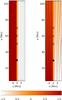Fig. 1 Vertical magnetic field component, By, (color map) for the gravity-free medium (left) and gravitationally stratified solar atmosphere (right). The magnetic field lines are displayed by solid lines. The full circles denote the location of the initial perturbation and crosses correspond to locations of detection points.

Figure 1 displays the vertical component of the magnetic field, B_y, for the gravity-free case (left panel) and for the gravitationally stratified solar corona (right panel). The magnetic field lines are expressed by full lines. Note that at x = 0 the vertical magnetic field component, B_y, experiences a sudden jump from negative (for x < 0) to positive values (for x > 0).

2.2.1. Gravity-free medium

In the gravity-free case, g =  [0,0,0] , we find that the magnetic field is ${B}\mathrm{=}\left[\mathrm{0}\mathit{,}{\mathit{B}}_{\mathrm{o}}\tanh \left(\frac{\mathit{x}}{{\mathit{w}}_{\mathrm{cs}}}\right)\mathit{,}\mathrm{0}\right]\mathit{.}$(11)This magnetic field corresponds to the Harris current-sheet. It changes from B₀ for high positive values of x to  − B₀ for high negative values of x, passing through zero at x = 0 (Fig. 1).

From the equation of static equilibrium, Eq. (8), we obtain the formula for the gas pressure distribution in the following form, see e.g. (Smith et al. 1997) $\mathit{p}\mathrm{\left(}\mathit{x,y}\mathrm{\right)}\mathrm{=}{\mathit{p}}_{\mathrm{CS}}\mathrm{·}{\mathrm{sech}}^{\mathrm{2}}\left(\frac{\mathit{x}}{{\mathit{w}}_{\mathrm{CS}}}\right)\mathit{,}$(12)where p_CS is the gas pressure at the center of the Harris current-sheet, expressed as ${\mathit{p}}_{\mathrm{CS}}\mathrm{=}{\mathit{n}}_{\mathrm{CS}}{\mathit{k}}_{\mathrm{B}}\mathit{T}\mathit{.}$(13)We assumed that in the equilibrium the plasma is isothermal with a temperature T = 10.0 × 10⁶ K (for the first studied case) or T = 5.0 × 10⁶ K (for the second studied case). The particle density in the center of the Harris current-sheet is n_CS = 4.0 × 10¹⁶ kg   m^-3 and k_B = 1.38 × 10^-23 J   K^-1 is the Boltzmann constant. After specifying gas pressure and temperature, we find the mass density distribution from the ideal gas law, $\mathit{\varrho }\mathrm{=}\frac{\mathit{mp}}{{\mathit{k}}_{\mathrm{B}}\mathit{T}}\mathrm{·}$(14)

2.2.2. Gravitationally stratified medium

To satisfy the solenoidal condition given by Eq. (5), combining it with Eq. (9) and using the gravitational acceleration that is oriented in the negative y-direction, g =  [0, − g_⊙,0] , we obtain the equations for the magnetic field in the x-y plane as ${\mathit{B}}_{\mathit{x}}\mathrm{\left(}\mathit{x,y}\mathrm{\right)}\mathrm{=}{\mathit{B}}_{\mathrm{o}}\frac{{\mathit{w}}_{\mathrm{cs}}}{\mathit{\lambda }}\ln \left[\cosh \left(\frac{\mathit{x}}{{\mathit{w}}_{\mathrm{cs}}}\right)\right]\exp \left(\mathrm{-}\frac{\mathit{y}}{\mathit{\lambda }}\right)\mathit{,}$(15)${\mathit{B}}_{\mathit{y}}\mathrm{\left(}\mathit{x,y}\mathrm{\right)}\mathrm{=}{\mathit{B}}_{\mathrm{o}}\tanh \left(\frac{\mathit{x}}{{\mathit{w}}_{\mathrm{cs}}}\right)\exp \left(\mathrm{-}\frac{\mathit{y}}{\mathit{\lambda }}\right)\mathrm{·}$(16)For details see Galsgaard & Roussev (2002).

In our 2D model without and with the gravity, Eq. (8) attains the following form: $\frac{\mathit{\partial p}\mathrm{\left(}\mathit{x,y}\mathrm{\right)}}{\mathit{\partial x}}\mathrm{+}{\mathit{j}}_{\mathit{z}}{\mathit{B}}_{\mathit{y}}\mathrm{\left(}\mathit{x,y}\mathrm{\right)}\mathrm{=}\mathrm{0}\mathit{,}$(17)$\frac{\mathit{\partial p}\mathrm{\left(}\mathit{x,y}\mathrm{\right)}}{\mathit{\partial y}}\mathrm{-}{\mathit{j}}_{\mathit{z}}{\mathit{B}}_{\mathit{x}}\mathrm{\left(}\mathit{x,y}\mathrm{\right)}\mathrm{+}\mathit{\varrho g}\mathrm{\left(}\mathit{x,y}\mathrm{\right)}\mathrm{=}\mathrm{0.}$(18)Here j_z is the only non-zero component of the electric current density j (see Eq. (6)), given by ${\mathit{j}}_{\mathit{z}}\mathrm{=}\frac{\mathrm{1}}{{\mathit{\mu }}_{\mathrm{0}}}\mathrm{(}\mathrm{\nabla }\mathrm{\times }{B}{\mathrm{)}}_{\mathit{z}}$.

The condition of integrability of the above equations leads to ${\mathit{\mu }}_{\mathrm{0}}\mathit{g}\frac{\mathit{\partial \varrho }\mathrm{\left(}\mathit{x,y}\mathrm{\right)}}{\mathit{\partial x}}\mathrm{=}\mathrm{\nabla }\mathrm{·}\mathrm{\left(}{\mathit{\mu }}_{\mathrm{0}}{\mathit{j}}_{\mathit{z}}{B}\mathrm{\right)}\mathit{,}$(19)from which we can derive the formulae for the distribution of the mass density $\begin{array}{ccc}\mathit{\varrho }\mathrm{\left(}\mathit{x,y}\mathrm{\right)}& \mathrm{=}& \{\frac{{\mathit{B}}_{\mathrm{o}}^{\mathrm{2}}}{{\mathit{\mu }}_{\mathrm{0}}\mathit{g\lambda }}\left\{\mathrm{1}\mathrm{+}\ln \left[\cosh \left(\frac{\mathit{x}}{{\mathit{w}}_{\mathrm{cs}}}\right)\right]\right\}{\mathrm{sech}}^{\mathrm{2}}\left(\frac{\mathit{x}}{{\mathit{w}}_{\mathrm{cs}}}\right)\\ & & \mathrm{+}{\mathit{\varrho }}_{\mathrm{0}}\}\exp \left(\mathrm{-}\mathrm{2}\frac{\mathit{y}}{\mathit{\lambda }}\right)\mathit{,}\end{array}$(20)and gas pressure $\begin{array}{ccc}\mathit{p}\mathrm{\left(}\mathit{x,y}\mathrm{\right)}& \mathrm{=}& \{\frac{{\mathit{B}}_{\mathrm{o}}^{\mathrm{2}}}{\mathrm{2}{\mathit{\mu }}_{\mathrm{0}}}{\mathrm{sech}}^{\mathrm{2}}\left(\frac{\mathit{x}}{{\mathit{w}}_{\mathrm{cs}}}\right)\mathrm{+}\frac{{\mathit{B}}_{\mathrm{o}}^{\mathrm{2}}{\mathit{w}}_{\mathrm{cs}}^{\mathrm{2}}}{\mathrm{2}{\mathit{\mu }}_{\mathrm{0}}{\mathit{\lambda }}^{\mathrm{2}}}{\ln }^{\mathrm{2}}\left[\cosh \left(\frac{\mathit{x}}{{\mathit{w}}_{\mathrm{cs}}}\right)\right]\\ & & \mathrm{+}\frac{{\mathit{\varrho }}_{\mathrm{0}}\mathit{g\lambda }}{\mathrm{2}}\}\exp \left(\mathrm{-}\mathrm{2}\frac{\mathit{y}}{\mathit{\lambda }}\right)\mathrm{+}{\mathit{p}}_{\mathrm{0}}\mathit{.}\end{array}$(21)Here ϱ₀ and p₀ are arbitrary integration constants. The corresponding plasma temperature is determined by Eq. (14).

2.3. Perturbations

At the start of the numerical simulation (t = 0 s), the equilibrium is perturbed by the Gaussian pulse in the x-component of velocity and has the following form (e.g. Nakariakov et al. 2004, 2005): ${\mathit{v}}_{\mathit{x}}\mathrm{=}\mathrm{-}{\mathit{A}}_{\mathrm{0}}\frac{\mathit{x}}{{\mathit{\lambda }}_{\mathit{y}}}\exp {\left[\mathrm{-}\frac{\mathrm{(}\mathit{x}\mathrm{-}{\mathit{L}}_{\mathrm{P}}\mathrm{)}}{{\mathit{\lambda }}_{\mathit{x}}}\right]}^{\mathrm{2}}\exp {\left[\mathrm{-}\frac{\mathit{y}}{{\mathit{\lambda }}_{\mathit{y}}}\right]}^{\mathrm{2}}\mathit{,}$(22)where A₀ is the initial amplitude of the pulse, and λ_x = λ_y = 1.0 Mm are the widths of the velocity pulse in the longitudinal and transverse directions, respectively. This pulse triggers preferentially fast magnetoacoustic sausage waves.

The perturbation point, L_P, in both the cases, is located on the axis of the current-sheet, at a distance of 30 Mm from the bottom boundary of the simulation region. The detection points, L_P, are also on the current-sheet axis and the distance between the perturbation and detection points is Δ ≡  | L_D − L_P |  = 20,30, and 40 Mm, respectively. See full black circles and crosses in Fig. 1.

3. Numerical model

The 2D time-dependent ideal MHD Eqs. (1)–(4) were solved numerically with the FLASH code. This code was initially developed to model nuclear flashes on the surfaces of neutron stars and white dwarfs, and the interior of white dwarfs; but it has since been applied to model a wide variety of astrophysical processes, see e.g. Fryxell et al. (2000). Currently, it is a well tested, fully modular, parallel, multiphysics, open science, simulation code that implements second- and third-order unsplit Godunov solvers and adaptive mesh refinement (AMR), see e.g. Chung (2002) and Murawski (2002). The Godunov solver combines the corner transport upwind method for multidimensional integration and the constrained transport algorithm for preserving the divergence-free constraint on the magnetic field (Lee & Deane 2009). In our case, the AMR strategy is based on controlling the numerical errors in a gradient of mass density that leads to reducing the numerical diffusion within the entire simulation region.

For our numerical simulations we used a 2D Eulerian box with the height and width of the simulation region; for all the studied cases, H = 100 Mm and W = 20 Mm, respectively (see Fig. 1). The spatial resolution of the numerical grid was determined with the AMR method and we used the AMR grid with the minimum (maximum) level of the refinement blocks set to 3 (7). Note that a spatial grid size has to be less than the typical width of the current-sheet along the x-direction and the typical wavelength of the magnetoacoustic waves along the y-direction, respectively. We found min(Δx) = 0.31 Mm and min(Δy) = 0.26 Mm, which satisfies the above mentioned condition (semi-width of the current-sheet is w_CS = 1.0 Mm and the estimated minimal wavelength is approximately 5.0 Mm). As a consequence of the real plasma medium extension we applied free-boundary conditions at the boundaries of the simulation region, so that the waves could freely leave the simulation box without any significant reflection.

4. Numerical results

We present the numerical results of evolution of fast magnetoacoustic sausage waves in the vertical current-sheet embedded in the gravitationally stratified solar atmosphere. Simultaneously, we compare these results with those obtained for the gravity-free case. Furthermore, we compare the numerical results in the gravitationally stratified solar atmosphere calculated for two different scale-heights. From wave signals detected at the three detection points we also compute the wavelet spectra and wave periods of obtained wavelet tadpoles.

For the wavelet analysis we used the Morlet wavelet, which consists of a plane wave modulated by a Gaussian, $\mathrm{\Psi }\mathrm{\left(}\mathit{t}\mathrm{\right)}\mathrm{=}{\mathit{\pi }}^{\mathrm{-}\mathrm{1}\mathit{/}\mathrm{4}}{\exp }^{\mathrm{\left(}\mathrm{i}\mathit{\sigma t}\mathrm{\right)}}{\exp }^{\mathrm{-}\mathrm{(}{\mathit{t}}^{\mathrm{2}}\mathit{/}\mathrm{2}\mathrm{)}}\mathit{,}$(23)where the parameter σ allows trade between time and frequency resolutions. Here we assumed the value of parameter σ = 6, as recommended by Farge (1992). The wave periods are estimated from the global wavelet spectrum as the most dominant period in this spectrum. More details about the wavelet method and its implementation can be found e.g. in Farge (1992) and Torrence & Compo (1998).

4.1. Gravity-free vs. gravitationally stratified solar atmosphere

In the following, in addition to the gravity-free current-sheet we consider the vertical current-sheet including gravity with two different scale-heights: the longer and shorter ones corresponding in the 1D gravity model to that with the temperature T = 10.0 × 10⁶ K and T = 5.0 × 10⁶ K, respectively. In the case with the longer scale-height we also study two cases with two different widths of the current-sheet.

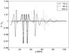Fig. 2 Profiles of the normalized mass density along the vertical axis (x = 0) of the current-sheet at times t = 10 s (solid line), 50 s (dashed line) and 100 s (dotted line) for the gravity-free case. The semi-width of the current-sheet is wCS = 1.0 Mm.

First, we compare the profiles of the normalized mass densities along the vertical axis of the current-sheet in the gravity-free case and gravitationally stratified plasma for a longer scale-height (Figs. 2 and 3). In Fig. 2 the normalized mass density in a gravity-free medium for times 10 s, 50 s, and 100 s is shown, while in Fig. 3 similar results are presented for the gravitationally stratified case for two widths of the current-sheet (in the left part for w_CS = 1.0 Mm and w_CS = 1.5 Mm in the right-hand side of the figure).

At the very early stage of the wave evolution, e.g. at t = 10 s (solid line), the wave has a very simple form in both cases. For longer times, t = 50 s and t = 100 s (dashed and dotted lines, respectively), some differences appear. The wave in the case of the gravitationally stratified solar atmosphere is slightly undulated and more irregular than in the gravity-free case. This effect seems to be caused by different wave dispersion in these two cases. Furthermore, in Fig. 3 one would expect that the wave amplitude will grow while the wave propagates toward lower mass densities, which occur at higher altitudes of the solar atmosphere. However, as can be seen here, the maximum amplitude decreases with height. This is caused by a relatively strong spatial dispersion of the wave pulse energy into larger and larger volume. Namely, different wave components of the initial wave pulse propagate with different group velocities and the wave pulse becomes longer in the vertical direction. Moreover, in this direction also the width of the current-sheet and thus the wave pulse becomes wider with an increase of y.

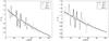Fig. 3 Profiles of the normalized mass density along the vertical axis of the current-sheet (x = 0) at times t = 10 s (solid line), 50 s (dashed line) and 100 s (dotted line) for the case of the gravity, longer scale-height and two semi-widths of the current-sheet wCS = 1.0 Mm (left) and wCS = 1.5 Mm (right).

We compare here also the incoming wave signals (expressed in relative plasma density variations) to the three selected detection points (Fig. 4) as well as the corresponding wavelet tadpoles (Fig. 5). In the left panels of both figures the results for the gravity-free current-sheet are shown. These results (wave periods as well as the wavelet tadpole shapes) look similar to those published by Jelínek & Karlický (2012). For comparison purposes, in the right columns we show the numerical results for the current-sheet that is embedded in the gravitationally stratified solar atmosphere.

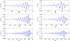Fig. 4 Incoming wave signals (expressed in relative plasma density variations) at the detection points LD = 50 Mm, 60 Mm, and 70 Mm (upper, middle, and lower panel, respectively). In the left column, the signals for the gravity-free case are shown; the signals detected in the gravitationally stratified solar atmosphere are presented in the right panel. The semi-width of the current-sheet is wCS = 1.0 Mm.

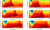Fig. 5 Temporal evolution of wavelet tadpoles for the three detection points: LD = 50 Mm, 60 Mm, and 70 Mm (upper, middle, and lower panel, respectively) for the gravity-free (left panels) and gravitationally stratified (right panels) solar atmosphere. The semi-width of the current-sheet is wCS = 1.0 Mm.

If we compare the numerical results displayed in Fig. 4, we can see that the wave signals propagating in the gravitationally stratified solar corona (right) have more irregular shapes than in the gravity-free case (left), which results from stronger wave dispersion in the former case. The arrival time of the “leading signal” is very similar in both cases because the mass density and the magnetic field in the vertical y-direction decreases in the same way, and thereforep the corresponding Alfvén speeds are approximately of the same magnitude.

As a result of the above mentioned irregularities in the incoming wave signals, which propagate in the gravitationally stratified solar atmosphere, we observe altered shapes of the wavelet tadpoles compared to the gravity-free case (Fig. 5).

The slightly different wave periods can also be discernible by comparing these two cases, as well as the different lengths of wavelet tadpoles. Nakariakov et al. (2005) found that narrower longitudinal drivers produce a broader k-spectrum above the cutoff for wave propagation in the waveguide, and accordingly, a broader interval of wave periods is detected. In our previous work (Jelínek & Karlický 2012) we verified these results for the Harris current-sheet by varying the current-sheet width. Therefore we conclude that the prolongation of the wave periods in the case of the gravitationally stratified solar corona results from the width of the current-sheet, which grows with heights (Fig. 1, right). This conclusion is also supported by the calculations performed for the two widths of the current-sheet, see Fig. 3, left part (narrower width) and right part (wider width of the current-sheet), where we verified that the wave period is directly proportional to the semi-width of the current-sheet in accordance with the relation provided by Roberts et al. (1984) $\mathit{P}\mathrm{\approx }\frac{\mathit{w}}{{\mathit{v}}_{\mathrm{Alf}}}\mathrm{·}$(24)

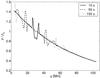Fig. 6 Profiles of the normalized mass density along the vertical axis of the current-sheet for (x = 0) at times t = 10 s (solid line), 50 s (dashed line) and 100 s (dotted line) for the gravitationally stratified plasma with the shorter scale-height. The semi-width of the current-sheet is wCS = 1.0 Mm.

4.2. Gravitationally stratified solar atmosphere

Figure 6 illustrates the same numerical results as Fig. 3, but for the shorter scale-height, corresponding in the 1D gravity model to the plasma temperature, T = 5.0 × 10⁶ K. The slope of the mass density in this case is steeper and the wave moves more slowly than in the case with the longer scale-height (Fig. 3). This corresponds to the fact that in this case the external Alfvén speed is slower than for the longer scale-height. Again at the very early stages t = 10 s (solid line) the wave has a simple form and later (50 and 100 s, dashed and dotted lines, respectively) it becomes undulated and irregular due to the wave dispersion.

Figure 7 displays incoming wave signals and corresponding wavelet tadpoles for the shorter scale-height to the three detection points. Comparing these signals with those in Fig. 4, we observe delays in the arrival times of the “leading signals”, which results from the lower value of the external Alfvén speed in this case, as mentioned in the previous paragraph. The estimated values of the arrival times of the “leading signals” to the detection points are presented in Table 1.

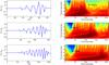Fig. 7 Comparison of the incoming signals (relative plasma density variations) and corresponding wavelet tadpoles at the three different detection points LD = 50 Mm, 60 Mm, and 70 Mm (upper, middle, and lower panel, respectively) in the case of the gravity and the shorter scale-height. The semi-width of the current-sheet is wCS = 1.0 Mm.

The forms of the wave signals are very similar and therefore there are no essential differences between the shapes of the wavelet tadpoles. On the other hand, if we compare the wave periods for both studied cases, we find that the wave period becomes longer for the shorter scale-height. This effect results from a lower value of the Alfvén speed and the ratios between the wave periods are approximately $\sqrt{\mathrm{2}}$.

Figures 4 and 7 show that the wave signal is more strongly attenuated in the case of the shorter scale-height. This is because the initial perturbation (which has the same initial amplitude in velocity) propagates in a denser environment than in the case of the longer scale-height. The denser environment here is due to the same value of the magnetic field in both studied cases, and consequently, according to Eq. (13), for the same pressure inside the current-sheet the shorter scale-height leads to the higher mass density.

Comparing Figs. 5 and 7 (right panels), we infer that the wavelet tadpoles become longer in the case of the shorter scale-height. Because we already verified the calculations given by Roberts et al. (1984) in our previous work for the Harris current-sheet, the time duration of the wavelet tadpole can be calculated as t_dp − t_ls, where t_dp =  | L_D − L_P | /v_A and ${\mathit{t}}_{\mathrm{ls}}\mathrm{=}\mathrm{|}{\mathit{L}}_{\mathrm{D}}\mathrm{-}{\mathit{L}}_{\mathrm{P}}\mathrm{|}\mathit{/}{\mathit{v}}_{\mathrm{gr}}^{\min }$ is the time of the decay phase and the arrival time of the “leading signal”, respectively (Jelínek & Karlický 2012). Hence, we conclude that longer lasting wavelet tadpoles result from a decrease in the group velocity. The group velocity in the case of the shorter scale-height is lower as a consequence of the higher mass density in the Harris current-sheet. As a result, the decay phase of the wave signal comes later than in the case of longer scale-height.

Figure 8 shows the contours of mass density for the longer and shorter scale-heights close to the area of the detection points (left parts of subfigures (a) and (b), respectively). In the right parts of these subfigures the selected zoomed parts of the mass densities are displayed. We also represent the vectors of the total velocity as black arrows. The results in Figs. 8a and b are displayed at time t = 100 s.

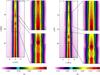Fig. 8 Spatial profiles of the mass density close to the area of the detection points with zoomed areas at t = 100 s for the case of the gravitationally stratified solar corona. The left part a) corresponds to the longer scale-height whereas the right part b) of the figure shows the area for the shorter scale-height. The black arrows represent the plasma velocity vectors. The mass density is expressed by colors which correspond to the ratio of the local mass density to that in the perturbation point, LP, in the initial time.

The initial Gaussian pulse in the horizontal component of the velocity generates the magnetoacoustic waves that perturb the equilibrium in the mass density. As a result, we observe the characteristic “sausage” structures after a sufficiently long time. In the case of the longer scale-height we see the structure with a longer wavelength than in the case with the shorter scale-height. These figures also show that the wave propagates faster in the case of the longer scale-height, as shown in Figs. 3 and 6, which display slices of these structures along the axes of the vertical flare current-sheet.

In the zoomed-in views of the mass density contours (right parts of Figs. 8a and b) the maxima and minima of wave amplitudes are displayed. They also show the vectors of the plasma flow velocities. We can see that there are inflows of the plasma in front of the propagating wave amplitude maxima, whereas on the rear side of these maxima the plasma is outflowing. As a result, the current-sheet is periodically narrowed and broadened according to the sausage wave structure.

5. Conclusions

By including gravity in our model, we made it more realistic than the previous models. We solved 2D time-dependent ideal MHD equations using the FLASH numerical code, implementing AMR (Lee & Deane 2009). We studied the propagation of magnetoacoustic waves in the vertical flare current-sheet in a gravitationally stratified solar atmosphere and for a gravity-free case. We compared the numerical results for two different scale-heights in the gravitationally stratified solar atmosphere.

We found several important differences between the studied cases. First, for the gravitationally stratified current-sheet it is necessary to implement additional horizontal component of the magnetic field, contrary to the gravity-free case. As a consequence of this modification, properties of the current-sheet such as the waveguide are changed. At the bottom part of the numerical box the parameters of the current-sheets are the same in both cases. However, in the gravity case the width of the current-sheet grows with height. This explains the longer wave periods of propagating magnetoacoustic waves in the gravitationally stratified solar atmosphere compared to the gravity-free case. Namely, the wave period is directly proportional to the width of the waveguide (current-sheet). The period is furthermore inversely proportional to the Alfvén speed, but this change is less important in this case.

By comparing the numerical results in the gravitationally stratified solar atmosphere we also found differences in the wave periods for the two different scale-heights. For the shorter scale-height case we found an even longer period, but here it is caused mainly by higher mass densities, i.e. by a lower Alfvén speed inside the waveguide. In this case also the minimal value of the group velocity is lower than in the case with longer scale-height. This explains the longer duration of the wavelet tadpoles.

However, these differences are mainly caused by the principal differences in the equilibrium current-sheet in the case with and without gravity. In addition to these differences we found that variations of the wave signal and their wavelet tadpoles are more irregular in the case with gravity than in the gravity-free case. We propose that these differences result from variations with height of the dispersive properties and group velocities of the propagating magnetoacoustic waves in the gravitational case.

The question arises how these results can be used for solar flare diagnostics. Obviously, the model of propagating fast magnetoacoustic sausage waves in the gravitationally stratified atmosphere is more realistic than that for the gravity-free case. The gravitationally stratified case allows us to make a direct comparison with observational data. The most frequently measurable parameters of these waves in solar events are periods and their temporal changes. For some events we can even compute the corresponding wavelet spectra with characteristic tadpoles. Combining these data with the possible determination of the wave types and their wavelengths (from positional measurements) together with independent estimates of the Alfvén speed at these locations (e.g. by the magnetic field extrapolation and UV and optical spectroscopy methods), we can directly compare the results of the present numerical modeling with the observational findings.

Furthermore, an improved description of the propagation of the fast sausage magnetoacoustic waves in waveguides (current-sheets or density enhancement regions) in the gravitationally stratified solar atmosphere can contribute to solving of the long-standing discussion about the origin of the so-called fiber (intermediate) bursts, (Young et al. 1961; Slottje 1981). Namely, there are several models of these bursts based on the whistler, Alfvén, and sausage magnetoacoustic waves (e.g. Bernold & Treumann 1983; Aurass et al. 1987; Mann et al. 1987; Kuznetsov 2006). However, there is still no clear evidence which types of waves are really present in radio sources of these bursts.

Acknowledgments

The authors P.J. and M.K. acknowledge support from the research project RVO:67985815 of the Astronomical Institute AS and Grants P209/10/1680 and P209/12/0103 of the Grant Agency of the Czech Republic. The author P. J. expresses his cordial thanks to Dr. J. Blažek for a discussion. This work has been supported by a Marie Curie International Research Staff Exchange Scheme Fellowship within the 7th European Community Framework Program (P. J. and K. M.). The FLASH code used in this work was in part developed by the DOE-supported ASC/Alliances Center for Astrophysical Thermonuclear Flashes at the University of Chicago. The wavelet analysis was performed using the software written by C. Torrence and G. Compo available at URL http://paos.colorado.edu/research/wavelets.

References

All Tables

All Figures

	Fig. 1 Vertical magnetic field component, By, (color map) for the gravity-free medium (left) and gravitationally stratified solar atmosphere (right). The magnetic field lines are displayed by solid lines. The full circles denote the location of the initial perturbation and crosses correspond to locations of detection points.
In the text

	Fig. 2 Profiles of the normalized mass density along the vertical axis (x = 0) of the current-sheet at times t = 10 s (solid line), 50 s (dashed line) and 100 s (dotted line) for the gravity-free case. The semi-width of the current-sheet is wCS = 1.0 Mm.
In the text

	Fig. 3 Profiles of the normalized mass density along the vertical axis of the current-sheet (x = 0) at times t = 10 s (solid line), 50 s (dashed line) and 100 s (dotted line) for the case of the gravity, longer scale-height and two semi-widths of the current-sheet wCS = 1.0 Mm (left) and wCS = 1.5 Mm (right).
In the text

Fig. 4 Incoming wave signals (expressed in relative plasma density variations) at the detection points LD = 50 Mm, 60 Mm, and 70 Mm (upper, middle, and lower panel, respectively). In the left column, the signals for the gravity-free case are shown; the signals detected in the gravitationally stratified solar atmosphere are presented in the right panel. The semi-width of the current-sheet is wCS = 1.0 Mm.

In the text

	Fig. 5 Temporal evolution of wavelet tadpoles for the three detection points: LD = 50 Mm, 60 Mm, and 70 Mm (upper, middle, and lower panel, respectively) for the gravity-free (left panels) and gravitationally stratified (right panels) solar atmosphere. The semi-width of the current-sheet is wCS = 1.0 Mm.
In the text

	Fig. 6 Profiles of the normalized mass density along the vertical axis of the current-sheet for (x = 0) at times t = 10 s (solid line), 50 s (dashed line) and 100 s (dotted line) for the gravitationally stratified plasma with the shorter scale-height. The semi-width of the current-sheet is wCS = 1.0 Mm.
In the text

	Fig. 7 Comparison of the incoming signals (relative plasma density variations) and corresponding wavelet tadpoles at the three different detection points LD = 50 Mm, 60 Mm, and 70 Mm (upper, middle, and lower panel, respectively) in the case of the gravity and the shorter scale-height. The semi-width of the current-sheet is wCS = 1.0 Mm.
In the text

Fig. 8 Spatial profiles of the mass density close to the area of the detection points with zoomed areas at t = 100 s for the case of the gravitationally stratified solar corona. The left part a) corresponds to the longer scale-height whereas the right part b) of the figure shows the area for the shorter scale-height. The black arrows represent the plasma velocity vectors. The mass density is expressed by colors which correspond to the ratio of the local mass density to that in the perturbation point, LP, in the initial time.

In the text

References

- Andries, J., Goossens, M., Hollweg, J. V., Arregui, I., & Van Doorsselaere, T. 2005, A&A, 430, 1109 [NASA ADS] [CrossRef] [EDP Sciences] [Google Scholar]
- Aschwanden, M. J., De Pontieu, B., Schrijver, C. J., & Alexander, D. 1999, ApJ, 520, 880 [NASA ADS] [CrossRef] [Google Scholar]
- Aurass, H., Chernov, G. P., Karlický, M., Kurths, J., & Mann, G. 1987, Sol. Phys., 112, 347 [NASA ADS] [CrossRef] [Google Scholar]
- Bernold, T. E. X., & Treumann, R. 1983, A&A, 264, 677 [Google Scholar]
- Chung, T. J. 2002, Computational Fluid Dynamics (New York, USA: Cambridge University Press) [Google Scholar]
- De Moortel, I., Ireland, J., & Walsh, R. W. 2000, A&A, 355, L23 [NASA ADS] [Google Scholar]
- De Moortel, I., Ireland, J., Walsh, R. W., & Hood, A. W. 2002, Sol. Phys., 209, 61 [NASA ADS] [CrossRef] [Google Scholar]
- Farge, M. 1992, Annu. Rev. Fluid Mech., 24, 395 [Google Scholar]
- Fryxell, B., Olson, K., Ricker, P., et al. 2000, ApJS, 131, 273 [NASA ADS] [CrossRef] [Google Scholar]
- Galsgaard, K., & Roussev, I. 2002, A&A, 383, 685 [NASA ADS] [CrossRef] [EDP Sciences] [Google Scholar]
- Jelínek, P., & Karlický, M. 2009, Eur. Phys. J. D, 54, 305 [NASA ADS] [CrossRef] [EDP Sciences] [Google Scholar]
- Jelínek, P., & Karlický, M. 2010, IEEE Trans. Plasma Sci., 38, 2243 [Google Scholar]
- Jelínek, P., & Karlický, M. 2012, A&A, 537, A46 [NASA ADS] [CrossRef] [EDP Sciences] [Google Scholar]
- Karlický, M., Jelínek, P., & Mészárosová, H. 2011, A&A, 529, A96 [NASA ADS] [CrossRef] [EDP Sciences] [Google Scholar]
- Katsiyannis, A. C., Williams, D. R., McAteer, R. T. J., et al. 2003, A&A, 406, 709 [NASA ADS] [CrossRef] [EDP Sciences] [Google Scholar]
- Kuznetsov, A. A. 2006, Sol. Phys., 237, 153 [NASA ADS] [CrossRef] [Google Scholar]
- Lee, D., & Deane, A. E. 2009, J. Comput. Phys., 228, 952 [NASA ADS] [CrossRef] [Google Scholar]
- Macnamara, C. K., & Roberts, B. 2010, A&A, 515, A41 [NASA ADS] [CrossRef] [EDP Sciences] [Google Scholar]
- Macnamara, C. K., & Roberts, B. 2011, A&A, 526, A75 [NASA ADS] [CrossRef] [EDP Sciences] [Google Scholar]
- Mann, G., Karlický, M., & Moschmann, U. 1987, Sol. Phys., 110, 381 [NASA ADS] [CrossRef] [Google Scholar]
- Mészárosová, H., Sawant, H. S., Cecatto, J. R., et al. 2009a, Adv. Space Res., 43, 1479 [NASA ADS] [CrossRef] [Google Scholar]
- Mészárosová, H., Karlický, M., Rybák, J., & Jiřička, K. 2009b, ApJ, 697, L108. [NASA ADS] [CrossRef] [Google Scholar]
- Murawski, K. 2002, Analytical and Numerical Methods for Wave Propagation in Fluid Media (Singapore: World Scientific) [Google Scholar]
- Murawski, K., & Roberts, B. 1994, Sol. Phys., 151, 305 [NASA ADS] [CrossRef] [Google Scholar]
- Nakariakov, V. M. 2003, in Dynamic Sun, ed. B. Dwiwedi (CUP) [Google Scholar]
- Nakariakov, V. M., & Verwichte, E. 2005, Liv. Rev. Sol. Phys., 2, 3 [Google Scholar]
- Nakariakov, V. M., Ofman, L., Deluca, E. E., Roberts, B., & Davilla, J. M. 1999, Science, 285, 862 [NASA ADS] [CrossRef] [PubMed] [Google Scholar]
- Nakariakov, V. M., Arber, T. D., Ault, C. E., et al. 2004, Mon. Not. R. Astron. Soc., 349, 705 [Google Scholar]
- Nakariakov, V. M., Pascoe, D. J., & Arber, T. D. 2005, Space Sci. Rev., 121, 115 [NASA ADS] [CrossRef] [Google Scholar]
- Ofman, L., & Wang, T. 2002, ApJ, 580, L85 [NASA ADS] [CrossRef] [Google Scholar]
- Ofman, L., Nakariakov, V. M., & DeForest, C. E. 1999, ApJ, 541, 441 [NASA ADS] [CrossRef] [Google Scholar]
- Pascoe, D. J., Nakariakov, V. M., & Arber, T. D. 2007, A&A, 461, 1149 [NASA ADS] [CrossRef] [EDP Sciences] [Google Scholar]
- Pascoe, D. J., Nakariakov, V. M., Arber, T. D., & Murawski, K. 2009, A&A, 494, 1119 [NASA ADS] [CrossRef] [EDP Sciences] [Google Scholar]
- Pascoe, D. J., Wright, A. N., & De Moortel, I. 2010, ApJ, 711, 990 [NASA ADS] [CrossRef] [Google Scholar]
- Priest, E. R. 1982, Solar Magnetohydrodynamics (London, England: D. Reidel Publishing Company) [Google Scholar]
- Roberts, B., Edwin, P. M., & Benz, A. O. 1983, Nature, 305, 688 [NASA ADS] [CrossRef] [Google Scholar]
- Roberts, B., Edwin, P. M., & Benz, A. O. 1984, ApJ, 279, 857 [NASA ADS] [CrossRef] [Google Scholar]
- Roberts, B. 2000, Sol. Phys., 193, 139 [NASA ADS] [CrossRef] [Google Scholar]
- Schrijver, C. J., Aschwanden, M. J., & Title, A. M. 2002, Sol. Phys., 206, 69 [NASA ADS] [CrossRef] [Google Scholar]
- Selwa, M., Murawski, K., & Solanki, S. K. 2005, A&A, 436, 701 [NASA ADS] [CrossRef] [EDP Sciences] [Google Scholar]
- Slottje, C. 1981, Atlas of Fine Structures of Dynamic Spectra of Solar Type-IV-dm and Some Type-II Radio Bursts (Dwingeloo, The Netherlands) [Google Scholar]
- Smith, J. M., Roberts, B., & Oliver, R. 1997, A&A, 327, 377 [NASA ADS] [Google Scholar]
- Thompson, B. J., Plunkett, S. P., Gurman, J. B., et al. 1998, Geophys. Res. Lett., 25, 2465 [Google Scholar]
- Torrence, Ch., & Compo, G. P. 1998, Bull. Am. Meteor. Soc., 79, 61 [Google Scholar]
- Wang, T. J., & Solanki, S. K. 2004, A&A, 421, L33 [NASA ADS] [CrossRef] [EDP Sciences] [Google Scholar]
- Young, C. W., Spencer, C. L., Moreton, G. E., & Roberts, J. A. 1961, ApJ, 133, 243 [NASA ADS] [CrossRef] [Google Scholar]
- Zaqarashvili, T. V., Oliver, R., & Ballester, J. L. 2005, A&A, 456, L13 [Google Scholar]