| Issue |
A&A
Volume 546, October 2012
|
|
|---|---|---|
| Article Number | A121 | |
| Number of page(s) | 14 | |
| Section | Stellar atmospheres | |
| DOI | https://doi.org/10.1051/0004-6361/201219747 | |
| Published online | 18 October 2012 | |
Radiative properties of magnetic neutron stars with metallic surfaces and thin atmospheres
1
Centre de Recherche Astrophysique de Lyon (CNRS, UMR 5574), Université Lyon
1, École Normale Supérieure de Lyon,
46 allée
d’Italie,
69364
Lyon Cedex 07,
France
e-mail: This email address is being protected from spambots. You need JavaScript enabled to view it.
2
Ioffe Physical-Technical Institute, Politekhnicheskaya 26, St. Petersburg
194021,
Russia
3
Isaac Newton Institute of Chile, St. Petersburg Branch,
Russia
4
Institut für Astronomie und Astrophysik, Kepler Center for Astro
and Particle Physics, Universität Tübingen, Sand 1, 72076
Tübingen,
Germany
5
Kazan Federal University, Kremlevskaja Str., 18, Kazan
420008,
Russia
6
Center for Relativistic Astrophysics, School of Physics, Georgia
Institute of Technology, Atlanta, Georgia
30332,
USA
Received:
4
June
2012
Accepted:
26
August
2012
Abstract
Context. Simple models fail to describe the observed spectra of X-ray-dim isolated neutron stars (XDINSs). Interpretating these spectra requires detailed studies of radiative properties in the outermost layers of neutron stars with strong magnetic fields. Previous studies have shown that the strongly magnetized plasma in the outer envelopes of a neutron star may exhibit a phase transition to a condensed form. In this case thermal radiation can emerge directly from the metallic surface without going through a gaseous atmosphere, or alternatively, it may pass through a “thin” atmosphere above the surface. The multitude of theoretical possibilities complicates modeling the spectra and makes it desirable to have analytic formulae for constructing samples of models without going through computationally expensive, detailed calculations.
Aims. The goal of this work is to develop a simple analytic description of the emission properties (spectrum and polarization) of the condensed, strongly magnetized surface of neutron stars.
Methods. We have improved our earlier work for calculating the spectral properties of condensed magnetized surfaces. Using the improved method, we calculated the reflectivity of an iron surface at magnetic field strengths B ~ 1012 G–1014 G, with various inclinations of the magnetic field lines and radiation beam with respect to the surface and each other. We constructed analytic expressions for the emissivity of this surface as functions of the photon energy, magnetic field strength, and the three angles that determine the geometry of the local problem. Using these expressions, we calculated X-ray spectra for neutron stars with condensed iron surfaces covered by thin partially ionized hydrogen atmospheres.
Results. We develop simple analytic descriptions of the intensity and polarization of radiation emitted or reflected by condensed iron surfaces of neutron stars with the strong magnetic fields typical of isolated neutron stars. This description provides boundary conditions at the bottom of a thin atmosphere, which are more accurate than previously used approximations. The spectra calculated with this improvement show different absorption features from those in simplified models.
Conclusions. The approach developed in this paper yields results that can facilitate modeling and interpretation of the X-ray spectra of isolated, strongly magnetized, thermally emitting neutron stars.
Key words: stars: neutron / stars: atmospheres / magnetic fields / radiation mechanisms: thermal / X-rays: stars
© ESO, 2012
1. Introduction
Recent observations of neutron stars have provided a wealth of valuable information, but they have also raised many new questions. Particularly intriguing is the class of radio-quiet neutron stars with thermal-like spectra, commonly known as X-ray dim isolated neutron stars (XDINSs), or the Magnificent Seven (see, e.g., reviews by Haberl 2007 and Turolla 2009, and references therein). Some of them (e.g., RX J1856.5−3754) have featureless spectra, whereas others (e.g., RX J1308.6+2127 and RX J0720.4−3125) have broad absorption features with energies ~0.2–2 keV. In recent years, an accumulation of observational evidence has suggested that XDINSs may have magnetic fields B ~ 1013–1014 G and be related to magnetars (e.g., Mereghetti 2008).
For interpretating the XDINS spectra, it may be necessary to take the phenomenon of “magnetic condensation” into account. The strong magnetic field squeezes the electron clouds around the nuclei, thereby increasing the binding and cohesive energies (e.g., Medin & Lai 2006, and references therein). Therefore XDINSs may be “naked,” with no appreciable atmosphere above a condensed surface, as first conjectured by Zane et al. (2002), or they may have a relatively thin atmosphere, with the spectrum of outgoing radiation affected by the properties of the condensed surface beneath the atmosphere, as suggested by Motch et al. (2003).
Reflectivities of condensed metallic surfaces in strong magnetic fields have been studied in several papers (Brinkmann 1980; Turolla et al. 2004; van Adelsberg et al. 2005; Pérez-Azorín et al. 2005). Brinkmann (1980) and Turolla et al. (2004) neglected the motion of ions in the condensed matter, whereas van Adelsberg et al. (2005; hereafter Paper I) and Pérez-Azorín et al. (2005) considered two opposite limiting cases, one that neglects the ion motion (“fixed ions”) and another where the ion response to the electromagnetic wave is treated by neglecting the Coulomb interactions between the ions (“free ions”). A large difference between these two limits occurs at photon frequencies below the ion cyclotron frequency, but the two models lead to almost the same results at higher photon energies. We expect that in reality the surface spectrum lies between these two limits (see Paper I for discussion). The results of Paper I and of Pérez-Azorín et al. (2005) are similar, but differ significantly from the earlier results. In particular, Turolla et al. (2004) find that collisional damping in the condensed matter leads to a sharp cutoff in the emission at low photon energies, but such a cutoff is absent in Paper I and Pérez-Azorín et al. (2005). It is most likely that this difference arises from the “one-mode” description for the transmitted radiation adopted by Turolla et al. (2004, see Paper I for details). All the previous works relied on a complicated method of finding the transmitted radiation modes, originally due to Brinkmann (1980). We replace it with the more reliable method described below.
Ho et al. (2007, see also Ho 2007) fitted multiwavelength observations of RX J1856.5−3754 with a model of a thin, magnetic, partially ionized hydrogen atmosphere on top of a condensed iron surface; they also discuss possible mechanisms of creation of such a thin atmosphere. Suleimanov et al. (2009) calculated various models of fully and partially ionized finite atmospheres above a condensed surface including the case of “sandwich” atmospheres, composed of hydrogen and helium layers above a condensed surface.
The wide variety of theoretical possibilities complicates the modeling and interpretation of the spectra. To facilitate this task, Suleimanov et al. (2010; hereafter Paper II) suggest an approximate treatment, in which the local spectra, together with temperature and magnetic field distributions, are fitted by simple analytic functions. By being flexible and fast, this approach is suited to constrain stellar parameters prior to performing more accurate, but computationally expensive calculations of model spectra. The reflectivity of the condensed surface was modeled by a simple steplike function, which roughly described the polarization-averaged reflectivity of a magnetized iron surface at B = 1013 G, but depended neither on the magnetic field strength B nor on the angle ϕ between the plane of incidence and the plane made by the normal to the surface and the magnetic field lines.
In the present work, the numerical method of Paper I and the approximate treatment of Paper II are refined. We develop a less complicated and more stable method of calculations and construct more accurate fitting formulae for the reflectivities of a condensed, strongly magnetized iron surface, taking the dependence on arguments B and ϕ into account. The new fit reproduces the feature near the electron plasma energy, obtained numerically in Paper I but neglected in Paper II. Two versions of the fit are presented in Sect. 2 for the models of free and fixed ions discussed in Paper I. In addition to the fit for the average reflectivity, we present analytic approximations for each of the two polarization modes, which allow us to calculate the polarization of radiation of a naked neutron star. In Sect. 3 we consider the radiative transfer problem in a finite atmosphere above the condensed surface, including the reflection from the inner atmosphere boundary with normal-mode transformations, neglected in the previous studies of thin atmospheres. Conclusions are given in Sect. 4. In Appendix A we describe the method of calculation for the reflectivity coefficients, which is improved with respect to Paper I. In Appendix B we describe an analytic model of normal-mode reflectivities at the inner boundary of a thin atmosphere.
2. Spectral properties of a strongly magnetized neutron star surface
2.1. Condensed magnetized surface
Most of the known neutron stars have much larger magnetic fields B than
the natural atomic unit for the field strength  G, which is set by
equating the electron cyclotron energy
G, which is set by
equating the electron cyclotron energy  (1)to the Hartree unit
of energy
mee4/ħ2.
Here, me is the electron mass, e the
elementary charge, c the speed of light in vacuum, ħ the Planck constant
divided by 2π, and
B13 = B/1013 G.
Fields with B ≫ B0 profoundly affect the
properties of atoms, molecules, and plasma (see, e.g., Haensel et al. 2007, Chap. 4). Ruderman
(1971) suggested that the strong magnetic field may stabilize linear molecular
chains (polymers) aligned with the magnetic field and eventually turn the surface of a
neutron star into the metallic solid state. Later studies have provided support for this
conjecture, although the surface density ρs and, especially,
the critical temperature Tcrit below which such condensation
occurs remain uncertain. Order-of-magnitude estimates suggest
(1)to the Hartree unit
of energy
mee4/ħ2.
Here, me is the electron mass, e the
elementary charge, c the speed of light in vacuum, ħ the Planck constant
divided by 2π, and
B13 = B/1013 G.
Fields with B ≫ B0 profoundly affect the
properties of atoms, molecules, and plasma (see, e.g., Haensel et al. 2007, Chap. 4). Ruderman
(1971) suggested that the strong magnetic field may stabilize linear molecular
chains (polymers) aligned with the magnetic field and eventually turn the surface of a
neutron star into the metallic solid state. Later studies have provided support for this
conjecture, although the surface density ρs and, especially,
the critical temperature Tcrit below which such condensation
occurs remain uncertain. Order-of-magnitude estimates suggest  (2)where A
and Z are the atomic mass and charge numbers, and η ~ 1
an unknown numerical factor, which absorbs the theoretical uncertainty (see Lai 2001). The value η = 1 corresponds
to the equation of state provided by the ion-sphere model (Salpeter 1954). More recent results of the zero-temperature Thomas-Fermi model
for 56Fe at
(2)where A
and Z are the atomic mass and charge numbers, and η ~ 1
an unknown numerical factor, which absorbs the theoretical uncertainty (see Lai 2001). The value η = 1 corresponds
to the equation of state provided by the ion-sphere model (Salpeter 1954). More recent results of the zero-temperature Thomas-Fermi model
for 56Fe at  G
(Fushiki et al. 1989; Rögnvaldsson et al. 1993) can be approximated (within 4%) by Eq. (2) with
G
(Fushiki et al. 1989; Rögnvaldsson et al. 1993) can be approximated (within 4%) by Eq. (2) with  , whereas
the finite-temperature Thomas-Fermi model of Thorolfsson
et al. (1998) does not predict magnetic condensation at all. The most
comprehensive study of cohesive properties of the magnetic condensed surface has been
conducted by Medin & Lai (2006, 2007), based on density-functional theory (DFT). Medin & Lai (2006) calculated cohesive energies
Qs of the molecular chains and condensed phases of H, He, C,
and Fe in strong magnetic fields. A comparison with previous DFT calculations by other
authors suggests that Qs may vary within a factor of two at
B ≳ 1012 G, depending on the approximations employed (see
Medin & Lai 2006, for references and
discussion). Medin & Lai (2007) calculated
equilibrium densities of saturated vapors of He, C, and Fe atoms and chains above the
condensed surfaces and obtained Tcrit at several values of
B by equating the vapor density to ρs.
Unlike previous authors, Medin & Lai (2006,
2007) have taken the electronic band structure of
the metallic phase into account self-consistently. However, in the gaseous phase, they
still did not allow for atomic motion across the magnetic field and did not take a
detailed treatment of excited atomic and molecular states into account. Medin & Lai (2007) calculated the surface
density assuming that the linear molecular chains (directed along
B) form a rectangular array in the perpendicular plane and
that the distance between the nuclei along the field lines is the same in the condensed
matter as in the separate molecular chain (Medin &
Lai 2006; Medin 2012, priv. comm.). Medin
& Lai (2007) found that the critical temperature is
Tcrit ≈ 0.08Qs/kB.
Their numerical results for 56Fe at
, whereas
the finite-temperature Thomas-Fermi model of Thorolfsson
et al. (1998) does not predict magnetic condensation at all. The most
comprehensive study of cohesive properties of the magnetic condensed surface has been
conducted by Medin & Lai (2006, 2007), based on density-functional theory (DFT). Medin & Lai (2006) calculated cohesive energies
Qs of the molecular chains and condensed phases of H, He, C,
and Fe in strong magnetic fields. A comparison with previous DFT calculations by other
authors suggests that Qs may vary within a factor of two at
B ≳ 1012 G, depending on the approximations employed (see
Medin & Lai 2006, for references and
discussion). Medin & Lai (2007) calculated
equilibrium densities of saturated vapors of He, C, and Fe atoms and chains above the
condensed surfaces and obtained Tcrit at several values of
B by equating the vapor density to ρs.
Unlike previous authors, Medin & Lai (2006,
2007) have taken the electronic band structure of
the metallic phase into account self-consistently. However, in the gaseous phase, they
still did not allow for atomic motion across the magnetic field and did not take a
detailed treatment of excited atomic and molecular states into account. Medin & Lai (2007) calculated the surface
density assuming that the linear molecular chains (directed along
B) form a rectangular array in the perpendicular plane and
that the distance between the nuclei along the field lines is the same in the condensed
matter as in the separate molecular chain (Medin &
Lai 2006; Medin 2012, priv. comm.). Medin
& Lai (2007) found that the critical temperature is
Tcrit ≈ 0.08Qs/kB.
Their numerical results for 56Fe at  can be described by expression
Tcrit ≈ (5 + 2 B13) × 105 K
for the critical temperature and by Eq. (2)
with η ≈ 0.55 for the surface density, with uncertainties below 20% for
both quantities. An observational determination of the phase state of a neutron star
surface would be helpful for improving the theory of matter in strong magnetic fields.
can be described by expression
Tcrit ≈ (5 + 2 B13) × 105 K
for the critical temperature and by Eq. (2)
with η ≈ 0.55 for the surface density, with uncertainties below 20% for
both quantities. An observational determination of the phase state of a neutron star
surface would be helpful for improving the theory of matter in strong magnetic fields.
The density of saturated vapor above the condensed surface rapidly decreases with decreasing T (Lai & Salpeter 1997). Therefore, although the surface is hidden by an optically thick atmosphere at T ≈ Tcrit, the atmosphere becomes optically thin at T ≪ Tcrit. Also, as suggested by Motch et al. (2003), there may be a finite amount of light chemical elements (e.g., H) on top of the condensed surface of a heavier element (e.g., Fe). In addition, the same atmosphere may be optically thick for low photon energies and transparent at high energies. The energy at which the total optical thickness of a finite atmosphere equals unity depends on the atmosphere column density, which can in turn depend on temperature. At a fixed energy, the optical thickness of the finite atmosphere is different for different photon polarizations, therefore the atmosphere can be thick for one polarization mode and thin for another. One should take all these possibilities into account while interpreting observed spectra of neutron stars.
2.2. Formation of the spectrum
2.2.1. Normal modes and polarization vectors
It is well known (e.g., Ginzburg 1970) that under typical conditions (e.g., far from the resonances) electromagnetic radiation propagates in a magnetized plasma in the form of extraordinary (X) and ordinary (O) normal modes. These modes have different polarization vectors eX and eO, absorption and scattering coefficients, and refraction and reflection coefficients at the surface. Gnedin & Pavlov (1973) studied conditions for the applicability of the normal-mode description and formulated the radiative transfer problem in terms of these modes.
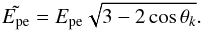
Following the works of Shafranov (1967) and
Ginzburg (1970), Ho & Lai (2001) derived convenient expressions for the normal mode
polarization vectors in a fully ionized plasma for photon energies E
much higher than the electron plasma energy  (3)where
ρ is the density in g cm-3. In the complex representation
of plane waves with
E ∝ e ei(k·r − ωt),
in the coordinate system where the z-axis is along the wave vector
k, and the magnetic field
B lies in the (xz) plane, the
polarization vectors are
(3)where
ρ is the density in g cm-3. In the complex representation
of plane waves with
E ∝ e ei(k·r − ωt),
in the coordinate system where the z-axis is along the wave vector
k, and the magnetic field
B lies in the (xz) plane, the
polarization vectors are  (4)We use the notation
M = X and M = O for the extraordinary and ordinary
polarization modes, respectively.
KM(α) and
Kz,M(α) are functions of
the angle α between B and
k. They are determined by the dielectric tensor of the
plasma and thus depend on the photon energy E, as well as
ρ, B, T and the chemical
composition. Ho & Lai (2003) calculated
KM and studied the polarization of normal
modes including the effect of the electron-positron vacuum polarization, while Potekhin et al. (2004) additionally considered an
incomplete ionization of the plasma.
(4)We use the notation
M = X and M = O for the extraordinary and ordinary
polarization modes, respectively.
KM(α) and
Kz,M(α) are functions of
the angle α between B and
k. They are determined by the dielectric tensor of the
plasma and thus depend on the photon energy E, as well as
ρ, B, T and the chemical
composition. Ho & Lai (2003) calculated
KM and studied the polarization of normal
modes including the effect of the electron-positron vacuum polarization, while Potekhin et al. (2004) additionally considered an
incomplete ionization of the plasma.
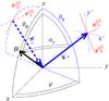 |
Fig. 1 Illustration of notations. The z axis is chosen perpendicular to
the surface, and the (xz) plane is chosen parallel to the
magnetic field lines, which make an
angle θB with the normal to the
surface. The direction of the reflected beam with wave vector
kr is determined by the polar
angle θk and the azimuthal
angle ϕ, and αr is the angle
between the reflected beam and the field lines. Thick solid lines show the
reflected beam and magnetic field directions, thin solid lines illustrate the
coordinates, and dashed lines show the incident photon wave vector
ki and its quadrant. The lines marked
|


2.2.2. Emission and reflection by a condensed surface
The condition
E > Epe is
usually satisfied for X-rays in neutron star atmospheres, but not in the condensed
matter. We consider a surface element that is sufficiently small for the variation in
the magnetic field strength and inclination to be neglected. We treat this small patch
as plane, neglecting its curvature and roughness. We choose the Cartesian
z axis perpendicular to this plane and the x axis
parallel to the projection of magnetic field lines onto the xy plane.
We denote the angle between the field and the z axis as
θB, the incidence angle of the radiation
as θk, and the angle in the
xy plane made by the projection of the wave vector as
ϕ (Fig. 1). The angle between
the wave vector and magnetic field lines is given by  (5)for the
incident and reflected waves, respectively. The surface emits radiation with
monochromatic intensities
(5)for the
incident and reflected waves, respectively. The surface emits radiation with
monochromatic intensities 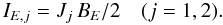 (6)Here, the basis for
polarization is chosen such that the waves with j = 1 and 2 are
linearly polarized parallel and perpendicular to the incident plane, respectively
(Fig. 1);
IE,j dΣ dΩ dE dt
gives the energy radiated in the jth wave by the surface element dΣ, in
the energy band (E,E + dE), during time
dt, in the solid angle element dΩ around the direction of the wave
vector k. We use the function
(6)Here, the basis for
polarization is chosen such that the waves with j = 1 and 2 are
linearly polarized parallel and perpendicular to the incident plane, respectively
(Fig. 1);
IE,j dΣ dΩ dE dt
gives the energy radiated in the jth wave by the surface element dΣ, in
the energy band (E,E + dE), during time
dt, in the solid angle element dΩ around the direction of the wave
vector k. We use the function
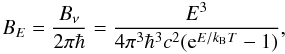 (7)where
Bν is Planck’s spectral radiance and
kB the Boltzmann constant. Dimensionless emissivities for
the two polarizations, normalized to blackbody values, are
Jj = 1 − Rj,
where Rj is the effective reflectivity of
mode j defined in Appendix A.
The reflectivities depend on surface material, photon energy, magnetic field strength
B and inclination θB,
and on the direction of k. For nonpolarized radiation, it
is sufficient to consider the mean reflectivity
R = (R1 + R2)/2
(see Paper I).
(7)where
Bν is Planck’s spectral radiance and
kB the Boltzmann constant. Dimensionless emissivities for
the two polarizations, normalized to blackbody values, are
Jj = 1 − Rj,
where Rj is the effective reflectivity of
mode j defined in Appendix A.
The reflectivities depend on surface material, photon energy, magnetic field strength
B and inclination θB,
and on the direction of k. For nonpolarized radiation, it
is sufficient to consider the mean reflectivity
R = (R1 + R2)/2
(see Paper I).
2.2.3. Reflectivity calculation
A method for calculating reflectivity coefficients was developed in Paper I. However, it is not easy to implement. Though it mostly produces correct results, in some ranges of model parameters it can yield unphysical results, which are difficult to distinguish from the correct ones. In the present work we present an improved method that avoids this complication (see Appendix A).
Using our new method, we calculated the spectral properties of a condensed Fe surface and compared the results with those in Paper I. As in Paper I, we considered two alternative models for the response of ions to electromagnetic waves in the condensed phase: one neglects the Coulomb interactions between ions, while the other treats ions as frozen at their equilibrium positions in the Coulomb crystal (i.e., neglecting their response to the electromagnetic wave).
In the first limiting case (thick lines in Fig. 2), the reflectivity exhibits different behavior in three characteristic energy
ranges: E < Eci,
 ,
and E ≳ EC, where
,
and E ≳ EC, where
 (8)is the
ion cyclotron energy, mu is the unified atomic mass unit,
and
(8)is the
ion cyclotron energy, mu is the unified atomic mass unit,
and  (9)In addition,
there is suppression of the reflectivity at
E ~ Epe; the exact position, width, and
depth of the suppression depend on the geometry defined by the angles
θB,
θk, and ϕ.
(9)In addition,
there is suppression of the reflectivity at
E ~ Epe; the exact position, width, and
depth of the suppression depend on the geometry defined by the angles
θB,
θk, and ϕ.
In the opposite case of immobile ions (thin curves in Fig. 2), the reflectivity has a similar behavior at E > Eci, but differs at E ≲ Eci. It does not exhibit the sharp change at E ≈ Eci, but smoothly continues to the lower energies. As argued in Paper I, we expect that the actual reflectivity lies between these two extremes.
The new results, shown in Fig. 2, display the same qualitative behavior as in Paper I, but exhibit considerable deviation from the previous calculations for some geometric settings in the energy range Eci ≲ E ≲ EC. Thus, the qualitative results and conclusions of Paper I are correct, but the new method described in Appendix A is quantitatively more reliable.
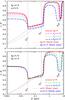 |
Fig. 2 Dimensionless emissivity J = 1 − R as a function of photon energy E for a condensed Fe surface with B = 1013 G and T = 106 K. The top panel shows several cases with varying θB and fixed θk = π/4, ϕ = π/4. The bottom panel shows several cases with varying ϕ and fixed θk = π/4, θB = π/4. These plots should be compared with Figs. 5 and 6 of Paper I. |
If
θB = θk = 0,
then an approximate analytic solution (neglecting the finite electron relaxation rate in
the medium; see Paper I for discussion) is
R ≈ (R + + R−)/2,
where ![Mathematical equation: \begin{equation} R_\pm^{(0)} = \left|\frac{n_\pm^{(0)}-1}{n_\pm^{(0)}+1}\right|^2, \quad n_\pm^{(0)} = \left[ 1 \pm \frac{\Epe^2}{\Ece(E\pm\Eci)} \right]^{1/2}\cdot \label{Rj0} \end{equation}](/articles/aa/full_html/2012/10/aa19747-12/aa19747-12-eq107.png) (10)Compared to the
numerical results, Eq. (10) provides a
good approximation at E ≲ Eci. Therefore,
we use it in the analytic fit described below.
(10)Compared to the
numerical results, Eq. (10) provides a
good approximation at E ≲ Eci. Therefore,
we use it in the analytic fit described below.
2.3. Results for iron surface
In the numerical examples presented below we assume a condensed 56Fe surface and use the estimate of the surface density given by the ion-sphere model – that is, we set η = 1 in Eq. (2).
2.3.1. Mean reflectivity
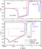 |
Fig. 3 Dimensionless emissivity J = 1 − R as a function of photon energy E for condensed Fe surface at B = 1013 G (top panel), B = 1012 G and 1014 G (bottom panel), with magnetic field lines normal to the surface, for two angles of incidence θk = 0 and θk = π/4, as marked near the curves. Solid lines show our numerical results, and dashed lines demonstrate the fit. For comparison, dotted lines reproduce the simplified approximation used in Paper II. |
In practice, the average normalized emissivity
J = 1 − R is usually more important than the
specific emissivities Rj. In Paper II,
R(E) was replaced by a constant in each of the three
ranges mentioned in Sect. 2.2.3
(E < Eci,
 , and
, and
 ).
For simplicity, the values of these three constants were assumed to depend only on
θB and
θk, but not on ϕ or
B. Here we propose a more elaborate and accurate fit, which is a
function of E, B,
θB,
θk, and ϕ, for the
magnetic field range 1012 G ≲ B ≲ 1014 G and
photon energy range 1 eV ≲ E ≲ 10 keV. In the approximation of free
ions, the average reflectivity of the metallic iron surface is approximately reproduced
by
).
For simplicity, the values of these three constants were assumed to depend only on
θB and
θk, but not on ϕ or
B. Here we propose a more elaborate and accurate fit, which is a
function of E, B,
θB,
θk, and ϕ, for the
magnetic field range 1012 G ≲ B ≲ 1014 G and
photon energy range 1 eV ≲ E ≲ 10 keV. In the approximation of free
ions, the average reflectivity of the metallic iron surface is approximately reproduced
by 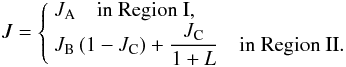 (11)Region I
is the low-energy region defined by the conditions
E < Eci and
JA > JB.
Region II is the supplemental range of relatively high energies in which either of these
conditions is violated. The functions JA,
JB, and JC are mainly
responsible for the behavior of the emissivity at
E < Eci,
(11)Region I
is the low-energy region defined by the conditions
E < Eci and
JA > JB.
Region II is the supplemental range of relatively high energies in which either of these
conditions is violated. The functions JA,
JB, and JC are mainly
responsible for the behavior of the emissivity at
E < Eci,
 ,
and
,
and  ,
respectively, while the function L describes the line at
E ≈ Epe. The value
,
respectively, while the function L describes the line at
E ≈ Epe. The value 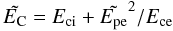 (12)is the
energy at which the square of the effective refraction index
(12)is the
energy at which the square of the effective refraction index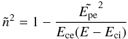 (13)(analogous
to Eq. (10)) becomes positive with
increasing E in the range
E > Eci. In
Eqs. (12) and (13),
(13)(analogous
to Eq. (10)) becomes positive with
increasing E in the range
E > Eci. In
Eqs. (12) and (13),
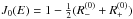
 (14)The low-energy part of
the fit in Eq. (11) is given by
(14)The low-energy part of
the fit in Eq. (11) is given by
![Mathematical equation: \begin{equation} J_\mathrm{A}=[1-A(E)]\,J_0(E), \end{equation}](/articles/aa/full_html/2012/10/aa19747-12/aa19747-12-eq130.png) (15)where
(15)where
![Mathematical equation: \begin{equation} A(E) = \frac{1-\cos\theta_B}{2\sqrt{1+B_{13}}}\, + \left[ 0.7-\frac{0.45}{J_0(0)}\, \right] \,(\sin\theta_k)^4\,(1-\cos\alpha), \label{A} \end{equation}](/articles/aa/full_html/2012/10/aa19747-12/aa19747-12-eq131.png) (16)
(16) , and
, and
 are
given by Eq. (10). Accordingly,
are
given by Eq. (10). Accordingly,
 .
In Eq. (16) and hereafter,
α without subscripts denotes
min(αr,αi).
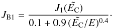
In the intermediate energy range,
.
In Eq. (16) and hereafter,
α without subscripts denotes
min(αr,αi).
In the intermediate energy range,  ,
there is a wide suppression of the emissivity. We describe this part by the power-law
interpolation between the values at Eci and
,
there is a wide suppression of the emissivity. We describe this part by the power-law
interpolation between the values at Eci and
 :
:
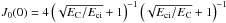
![Mathematical equation: \begin{equation} J_\mathrm{B} = (E/\tilde\EC)^p J(\tilde\EC), \quad\textrm{where~~} p=\frac{\ln[J(\tilde\EC)/J(\Eci)]}{\ln(\tilde\EC/\Eci)}\cdot \label{JB} \end{equation}](/articles/aa/full_html/2012/10/aa19747-12/aa19747-12-eq139.png) (17)The values
J(Eci) and
(17)The values
J(Eci) and
 are approximated as
follows:
are approximated as
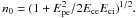
follows: 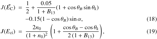 where
where
 The steep slope at
is described by Eq. (10) with
Epe replaced by
The steep slope at
is described by Eq. (10) with
Epe replaced by  :
:
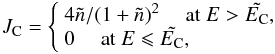 (20)
(20) being given by Eq. (13).
Finally, the lowering of J(E) at
is fit by ![Mathematical equation: \begin{eqnarray} \label{L} {L} &=& \left[ \frac{0.17\Epe/\EC }{1+X^4} +0.21\,\mathrm{e}^{-(E/\Epe)^2} \right] (\sin\theta_k)^2\,W_L, \\ X &= & \frac{E-E_L}{2\Epe W_L}\,(1-\cos\theta_k)^{-1}, \nonumber\\ E_L&=&\Epe\left[ 1+1.2\,(1-\cos\theta_k)^{3/2} \right] \,\left[ 1-(\sin\theta_B)^2/3 \right], \nonumber\\ W_L &=& 0.8\,(\tilde\EC/\Epe)^{0.2} \sqrt{\sin(\alpha/2)}\, \left[ 1+(\sin\theta_B)^2 \right]. \nonumber \end{eqnarray}](/articles/aa/full_html/2012/10/aa19747-12/aa19747-12-eq149.png) (21)The
line at EL disappears from the fit
(L → 0) when radiation is parallel to the magnetic field
(α → 0). This property is not exact; our numerical results reveal a
remnant of the line at α → 0, which is relatively weak, but may become
appreciable if the magnetic field is strongly inclined
(θB > π/4).
(21)The
line at EL disappears from the fit
(L → 0) when radiation is parallel to the magnetic field
(α → 0). This property is not exact; our numerical results reveal a
remnant of the line at α → 0, which is relatively weak, but may become
appreciable if the magnetic field is strongly inclined
(θB > π/4).
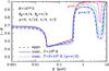 |
Fig. 4 Dimensionless emissivity J = 1 − R as a function of photon energy E for a condensed Fe surface with inclined magnetic field (B = 1013 G, θB = π/4) and inclined incidence of radiation (θk = π/4 and four values of ϕ listed in the figure). Solid lines show our numerical results for the model of free ions at T = 106 K, and short-dashed lines demonstrate the fit. For comparison, the dotted line reproduces our numerical results for ϕ = π/2 and T = 3 × 10⁵ K. |
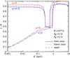 |
Fig. 5 Same as in Fig. 4, but for B = 1014 G and two values of ϕ. For comparison, the dotted and long-dashed lines reproduce our numerical results and analytic approximation, respectively, for the model of fixed ions. |
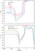 |
Fig. 6 Dimensionless emissivity for the linear polarization e1, J1 = 1 − R1, as a function of photon energy E for condensed Fe surface at different magnetic field strengths and geometric settings. Top panel: magnetic field B = 1013 G is normal to the surface, and angles of radiation incidence are θk = 0, π/6, π/4, and π/3. Bottom panel: B = 1013.5 G, magnetic field lines and the photon beam are both inclined at θB = θk = π/4, and the azimuthal angle takes values ϕ = 0, π/4, and π/2. Solid lines show the numerical results, and dashed lines demonstrate the fit. |
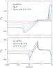 |
Fig. 7 Degree of linear polarization Plin (Eq. (28)) as a function of photon energy E for condensed Fe surface. The values of B, directions of the field and the wave vector, and line types are same as in Fig. 6. |
Examples of the numerical results for the normalized emissivities are compared to the analytic approximation in Figs. 3–5. For most geometric settings, the fit error lies within 10% in more than 95% of the interval −3 < log 10E(keV) < 1. The remaining <5% are the narrow ranges of E where J(E) sharply changes. Exceptions occur for strongly inclined fields (θB > π/4) and small ϕ, where the error may exceed 20% in up to 10% of the logarithmic energy range.
Our fit does not take the dependence of reflectivity on temperature into account. Temperature of the condensed matter enters in the calculations through the effective relaxation time, which determines the damping factor (see Paper I). This disregard is justified by the weakness of the T-dependence of the results. With decreasing T, the transitions of R(E) between characteristic energy ranges become sharper, and the feature at EL becomes stronger. The bulk of our calculations employed in the fitting was done at T ~ 106 K. In Fig. 4, which shows the numerical results at T = 106 K, an additional line is drawn at T = 3 × 10⁵ K, in order to illustrate the T-dependence.
A small modification of the proposed approximation can describe the alternative model
of fixed ions (see Paper I). In this case, it is sufficient to formally set
Eci → 0 in the above equations and replace Eq. (17) by 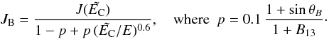 (22)As an example, in
Fig. 5 the numerical results in the model of
fixed ions and the fit Eq. (22) are
shown in addition to the free-ion results.
(22)As an example, in
Fig. 5 the numerical results in the model of
fixed ions and the fit Eq. (22) are
shown in addition to the free-ion results.
2.3.2. Polarization
We also constructed approximations for the emissivities in each of the two modes. Their
functional dependence on E and geometric angles in Fig. 1 is more complicated than the analogous dependence for
the average
J = (J1 + J2)/2.
We did not accurately reproduce these complications, in order to keep the fit relatively
simple, but reproduced general trends. For j = 1, our free-ion
approximation has the same form as Eq. (11): 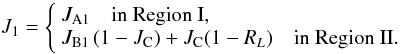 (23)Here,
we retain JC given by Eq. (20). The shape of the line near the plasma frequency is unchanged
and is described by Eq. (21), but the
line strength is different, since L enters Eq. (23) through the function
(23)Here,
we retain JC given by Eq. (20). The shape of the line near the plasma frequency is unchanged
and is described by Eq. (21), but the
line strength is different, since L enters Eq. (23) through the function
![Mathematical equation: \begin{eqnarray} R_L &=& (\sin\theta_B)^{1/4}\,\left[2-(\sin\alpha)^4 \right] \,\frac{{L}}{1+{L}} \cdot \end{eqnarray}](/articles/aa/full_html/2012/10/aa19747-12/aa19747-12-eq176.png) (24)The
functions that describe emissivity in mode 1 at
(24)The
functions that describe emissivity in mode 1 at  are
are ![Mathematical equation: \begin{eqnarray} J_\mathrm{A1} &=& [ 1 - A_1 ] \, J_\mathrm{A}, \\ A_1 &=& \frac{a_1}{1+0.6\,B_{13}\,(\cos\theta_B)^2}, \nonumber\\ a_1 &=& 1-(\cos\theta_B)^2\cos\theta_k-(\sin\theta_B)^2\cos\alpha; \nonumber\\ J_\mathrm{B1} &=& (E/\tilde\EC)^{p_1} J_1(\tilde\EC), \qquad p_1=\frac{\ln[J_1(\tilde\EC)/J_1(\Eci)]}{\ln(\tilde\EC/\Eci)}, \label{JB1}\\ J_1(\Eci) &=& (1-a_1)\,J(\Eci), \nonumber\\ J_1(\tilde\EC) &=& \frac12 + \frac{0.05}{1+B_{13}}+\frac{\sin\theta_B}{4}\cdot \nonumber \end{eqnarray}](/articles/aa/full_html/2012/10/aa19747-12/aa19747-12-eq178.png) In
the fixed-ion case, it is sufficient to set Eci → 0 and to
replace Eq. (26) by
In
the fixed-ion case, it is sufficient to set Eci → 0 and to
replace Eq. (26) by
 (27)For the second mode, no
additional fitting is needed, because
R2 = 2R − R1
and
J2 = 2J − J1.
(27)For the second mode, no
additional fitting is needed, because
R2 = 2R − R1
and
J2 = 2J − J1.
Figure 6 compares the use of Eqs. (23)–(26) to numerical results. The upper panel shows the case where the
field lines are perpendicular to the surface. In this case the line at
EL disappears from mode 1, so the line in
R seen in Fig. 3 for
θk ≠ 0 is entirely due to mode 2. As soon
as the field is inclined, the line is redistributed between the two modes (the lower
panel of Fig. 6). In the latter case the numerical
results show a more complex functional dependence
R1(E) in the range
 ,
which is not fully reproduced by our fit, for the reasons discussed above.
,
which is not fully reproduced by our fit, for the reasons discussed above.
The azimuthal angle ϕ enters the fit only through α. As a consequence, the fit is symmetric with respect to a change in sign of ϕ. This property may seem natural at first glance; however, we note that the numerical results do not strictly obey this symmetry, which holds for the nonpolarized beam, but not for each of the polarization modes separately. We have checked that this is not a numerical artifact: because the magnetic field vector B is axial, there is no strict symmetry with respect to the (x,z) plane. A reflection about this plane would require simultaneous inversion of the B direction in order to restore the original results. However, as long as the electromagnetic waves are nearly transverse (i.e., Kz in (4) and (A.24) are small), the asymmetry is weak, allowing us to ignore it and thus keep the fit relatively simple.
The analytic approximations in Eqs. (11) and (23) allow one to
evaluate the degree of linear polarization of the emitted radiation  (28)For example, the two
panels of Fig. 7 show
Plin for the same directions of the magnetic field and the
photon beam as in the respective panels of Fig. 6.
We see that the analytic formulae, originally devised to reproduce the normalized
emissivities, also reproduce the basic features of
Plin(E). Although the feature at
E ~ Epe is absent in the top panel of
Fig. 6, it reappears in the top panel of
Fig. 7 due to the contribution of
R2 in Eq. (28).
(28)For example, the two
panels of Fig. 7 show
Plin for the same directions of the magnetic field and the
photon beam as in the respective panels of Fig. 6.
We see that the analytic formulae, originally devised to reproduce the normalized
emissivities, also reproduce the basic features of
Plin(E). Although the feature at
E ~ Epe is absent in the top panel of
Fig. 6, it reappears in the top panel of
Fig. 7 due to the contribution of
R2 in Eq. (28).
3. X-ray spectra of thin atmospheres
3.1. Inner boundary conditions
Propagation of radiation in an atmosphere is described by two normal modes (see
Sect. 2.2.1). At the inner boundary of a thin
atmosphere, an incident X-mode beam of intensity  gives rise to
reflected beams in both modes, whose intensities are proportional to
, and
analogously for an incident O-mode. Therefore, the inner boundary conditions for radiation
transfer in an atmosphere of a finite thickness above the condensed surface can be written
as
gives rise to
reflected beams in both modes, whose intensities are proportional to
, and
analogously for an incident O-mode. Therefore, the inner boundary conditions for radiation
transfer in an atmosphere of a finite thickness above the condensed surface can be written
as 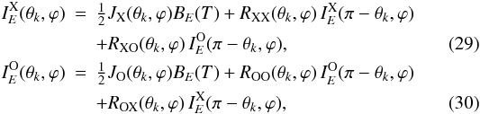 where
where
 (M = X,O) are the specific intensities of the X- and
O-modes in the atmosphere at ρ = ρs,
RMM′ are
coefficients of reflection with allowance for transformation of the incident mode
M′ into the reflected mode M, and
JM are the normalized emissivities. The
latter can be written by analogy with J1,2 as
JX = 1 − RX and
JO = 1 − RO, where
RX = RXX + RXO
and
RO = ROO + ROX
(cf. Paper I).
(M = X,O) are the specific intensities of the X- and
O-modes in the atmosphere at ρ = ρs,
RMM′ are
coefficients of reflection with allowance for transformation of the incident mode
M′ into the reflected mode M, and
JM are the normalized emissivities. The
latter can be written by analogy with J1,2 as
JX = 1 − RX and
JO = 1 − RO, where
RX = RXX + RXO
and
RO = ROO + ROX
(cf. Paper I).
Ho et al. (2007) retained only the emission terms
 on the right-hand
sides of Eqs. (29), (30). The reflection was taken into account in
Paper II, but calculations were performed neglecting ROO,
ROX, and RXO, under the
assumption that RXX is equal to R and does
not depend on ϕ. Here we use a more realistic, albeit still approximate,
model for RMM′,
described in Appendix B.
on the right-hand
sides of Eqs. (29), (30). The reflection was taken into account in
Paper II, but calculations were performed neglecting ROO,
ROX, and RXO, under the
assumption that RXX is equal to R and does
not depend on ϕ. Here we use a more realistic, albeit still approximate,
model for RMM′,
described in Appendix B.
3.2. Results
Here, we illustrate the importance of the correct description of the reflection for computations of thin model atmospheres above a condensed surface. To this end, we have calculated a few model atmospheres with normal magnetic field (therefore, θB = ϕ = 0, and αr = αi = θk), taking the model with B = 4 × 10¹³ G, effective temperature Teff = 1.2 × 10⁶ K, and surface density Σ = 10 g cm-2 as a fiducial model. In the fiducial model the free-ions assumption for condensed-surface reflectivity is used.
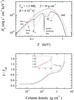 |
Fig. 8 Emergent spectra (top panel) and temperature structures (bottom panel) for the fiducial model atmosphere (solid curve) and for model atmospheres that are calculated using the fixed-ions approximation for the reflectivity calculations (dashed curves), and the inner boundary condition from Paper II (dotted curves). In the top panel the diluted blackbody spectrum that fits the high-energy part of the fiducial model spectrum is also shown (dash-dotted curve). |
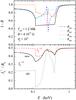 |
Fig. 9 Top panel: dimensionless emissivities for coefficients of reflection RXX (dashed curve), RXO (dotted curve), ROX (dash-dot-dotted curve), and ROO (dash-dotted curve). The quantities are calculated at the bottom of the fiducial model atmosphere for the angle between the radiation propagation and magnetic field, θk = 10°, together with the total dimensionless emissivity (solid curve). Bottom panel: dimensionless outward specific intensities (inner boundary condition) at the bottom of the fiducial model atmosphere for the X-mode (solid curve) and O-mode (dashed curve). For comparison, the dotted curve shows the same for the X-mode, calculated using the inner boundary condition from Paper II (in this case the dimensionless specific intensity of the O-mode equals 0.5). |
For these computations we use the numerical code described in Suleimanov et al. (2009), with a modified iterative procedure for
temperature corrections. We evaluate these corrections using the Unsöld-Lucy method (e.g.,
Mihalas 1978), which gives a better convergence
for thin-atmosphere models than other standard methods. In our case, the deepest
atmosphere point is the upper point of the condensed surface. The temperature correction
at this point is obtained as follows: the total flux at the boundary between the
atmosphere and the condensed surface is fixed and, therefore, the following energy balance
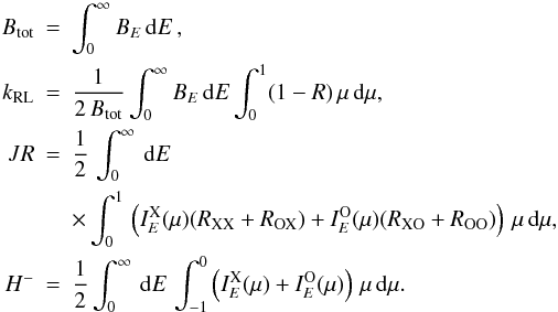
condition has to be satisfied: 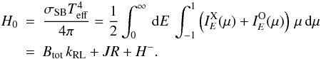 (31)Here,
σSB is the Stefan-Boltzmann constant,
μ = cosθk, and
(31)Here,
σSB is the Stefan-Boltzmann constant,
μ = cosθk, and
 (32)Generally,
the condition (31) is not fulfilled at a
given temperature iteration. Therefore, we perform a linear expansion of the integrated
blackbody intensity:
(32)Generally,
the condition (31) is not fulfilled at a
given temperature iteration. Therefore, we perform a linear expansion of the integrated
blackbody intensity:  (33)and find a
corresponding temperature correction
(33)and find a
corresponding temperature correction 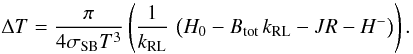 (34)This last-point
correction procedure is stable and has a convergence rate similar to the Unsöld-Lucy
procedure at other depths.
(34)This last-point
correction procedure is stable and has a convergence rate similar to the Unsöld-Lucy
procedure at other depths.
We also changed the depth grid for a better description of the temperature structure in thin-atmosphere models. In semi-infinite model atmospheres that do not have a condensed surface as a lower boundary, a logarithmically equidistant set of depths is used. However, in thin-atmosphere models, such a set yields insufficient accuracy at the boundary between the atmosphere and condensed surface. To improve the description of the boundary, we divide the model atmosphere into two parts with equal thicknesses and use logarithmically equidistant depth grids for each of them. In the upper part the grid starts from outside (the closest points are at the smallest depths), while in the lower part it starts from the condensed surface (the closest points are at the deepest depths). This combined grid allows us to describe the whole atmosphere with the desired accuracy of 1% for the integral flux conservation.
In Fig. 8 we show the emergent spectra and temperature structures for three different model atmospheres with the same fiducial set of physical parameters. The model spectrum computed using the inner boundary condition described in Paper II (the “old model”) significantly differs from the two other model spectra computed using the improved boundary conditions of Eqs. (29), (30). The latter two models are calculated using the free (fiducial model) and fixed ions (alternative model) assumptions for the condensed surface reflectivities.
The differences between the spectra and the temperature structures of these two models are very small. The atmosphere temperature near the condensed surface with fixed ions is slightly smaller than the temperature near the condensed surface with free ions. The flux in the spectrum of the fiducial model is approximately twice that of the alternative model at photon energies E smaller than the iron cyclotron energy Eci = 0.118 keV. At larger energies the spectra are very close to each other. We note that the old model has been computed using the free-ions assumption.
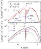 |
Fig. 11 Top panel: total emergent spectrum of the fiducial model (solid curve), together with emergent spectra in the X-mode (dashed curve) and in the O-mode (dash-dotted curve). The blackbody spectrum with T = Teff is also shown (dotted curve). Bottom panel: emergent specific intensities of the fiducial model for six angles θ. |
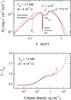 |
Fig. 12 Comparison of emergent spectra (top panel) and temperature structures (bottom panel) of the fiducial model (solid curves) with the semi-infinite model atmosphere (dashed curves) and with the thinner (Σ = 1 g cm-2) model atmosphere (dotted curves), but with the same magnetic field. |
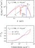 |
Fig. 13 Comparison of emergent spectra (top panel) and temperature structures (bottom panel) of the fiducial model (solid curves) and the model atmosphere with different magnetic field (B = 1014 G), but with the same surface density (dashed curves). |
The difference in the emergent spectra between the old and new model atmospheres is significant. In the old model, there is a deep depression of the spectrum between Eci and EC with an emission-like feature around the absorption line at the proton cyclotron energy Ecp = 0.252 keV. In the new spectra this complex feature between Eci and EC is completely different. The total depression is not significant, but instead of the flux increase, there appears a deep absorption feature at photon E ≳ Ecp. This absorption corresponds to the bound-bound transitions in hydrogen atoms in strong magnetic field (Hb−b feature).
It is clear that this difference arises due to the inner boundary condition. The bottom panels of Figs. 9 and 10 illustrate the difference in the outgoing flux at the boundary between the atmosphere and the condensed surface for the old and new models. This difference is especially large for the flux in the X-mode. In the old model we assumed complete reflection in the X-mode; therefore, the reflected flux was small as the atmosphere was optically thin at these energies. As a result we found a small emergent flux at these energies. In the new models, we have significant mode transformation due to reflection, which causes an appreciable part of the energy from the O-mode to convert into the X-mode; the converted photons then almost freely escape from the atmosphere. The reflectivity coefficients RMM′ for two angles θk are shown in the upper panels of Figs. 9 and 10.
The total equivalent widths (EWs) of the complex absorption features in the spectra of the new models are smaller than the EW of this feature in the spectrum of the old model. Nevertheless, they are still significant, with EW ≈ 220−250 eV, if the continuum is assumed to be a diluted blackbody spectrum that fits the high-energy tail of the model. The parameters of the diluted blackbody spectrum are a color correction factor fc = T/Teff = 1.2, and a dilution factor D = 1.1-4. The range of values for EW is sufficient to explain the observed absorption features of XDINSs (for reviews, see Haberl 2007; Turolla 2009).
The new and old spectra are strongly polarized, with most of the energy radiated in the X-mode (see Fig. 11, upper panel). We note that, for the parameters of the fiducial model, the vacuum resonance density occurs between the X and O mode photon decoupling densities. Therefore, the polarization signal does not exhibit a rotation of the plane of polarization between low and high energies. In contrast, models that exhibit this effect, considered by Lai & Ho (2003) and van Adelsberg & Lai (2006), have a lower magnetic field and higher effective temperature, causing the vacuum resonance to occur outside the X and O photospheres.
The angular distribution of the emergent flux is different in the two models (Fig. 11, bottom panel), especially at photon energies between EC and 4EC. In the old model, the angular distribution is peaked around the surface normal. In the new model, the emergent radiation is almost isotropic, with a peak around the surface normal at the broad Hb−b absorption feature.
The influence of the atmosphere thickness on its emergent spectrum and the temperature structure is illustrated in Fig. 12. A thinner atmosphere with Σ = 1 g cm-2 has an insignificant Hb−b absorption feature because it is formed at higher column densities (≈1–2 g cm-2). The fiducial model has the smallest temperature at these column densities among all the models. As a result, the Hb−b absorption feature is most significant in the spectrum of this model. The spectrum of the semi-infinite atmosphere has a hard tail and does not have any feature at Eci.
The importance of the Hb−b absorption feature decreases if it is located far from the maximum of the spectrum. This is illustrated by the comparison of the fiducial model with the model calculated for B = 1014 G (Fig. 13). In the latter case, the Hb−b absorption feature is less visible and cools the atmosphere at column densities about a few g cm-2 less efficiently, although the EW decreases insignificantly.
3.3. Discussion: toward models of observed spectra
Our calculations are presented for a local patch of the neutron-star surface with particular values of Teff and B. By taking surface distributions of Teff and B into account, one can construct an emission spectrum from the entire neutron star; however this spectrum is necessarily model-dependent, as the Teff and B distributions are generally unknown. If these distributions are sufficiently smooth, then integration over the surface makes absorption features broader and shallower, as demonstrated, e.g., in the case of cooling neutron stars with dipole magnetic fields and semi-infinite (Ho et al. 2008) or thin (Paper II) partially ionized hydrogen atmospheres. As shown in Paper II, smearing of the features is stronger, if the crustal magnetic field has a strong toroidal component, but weaker, if radiation is formed at small hotspots on the surface, where B can be considered as constant. Using the results of Paper II, Hambaryan et al. (2011) fitted observed phase-resolved spectra of XDINS RBS 1223 and derived constraints on temperature and magnetic field strength and distribution in the X-ray emitting areas, their geometry, and the gravitational redshift at the surface. The present, more detailed approximations for the reflectivities can be directly used to refine these fits and constraints.
In our numerical examples presented above, we evaluated the density of the condensed
matter using Eq. (2) with
η = 1. An eventual correction to this approximation is rather
straightforward, once ρs is accurately known. Indeed, the
density enters calculations through  (Eq. (3)) and through the damping factor
(Paper I). The latter dependence is relatively weak, therefore, it is sufficient to
correct Epe in the expressions presented in Sect. 2.
(Eq. (3)) and through the damping factor
(Paper I). The latter dependence is relatively weak, therefore, it is sufficient to
correct Epe in the expressions presented in Sect. 2.
As mentioned in Sect. 3.2, the model spectra are highly polarized at the stellar surface. However, the observed polarization signal is affected by propagation of the photons through the neutron-star magnetosphere. In addition to redshift and light bending effects near the stellar surface, the mode eigenvectors evolve adiabatically along with the direction of the changing magnetic field in the magnetosphere (see, e.g., Heyl & Shaviv 2002). The adiabatic evolution continues until the photons near the polarization limiting radius, rpl, which is typically many stellar radii from the surface. At rpl, the modes couple, with the intensities and eigenvectors frozen thereafter (in addition, significant circular polarization can be generated in some cases, for example, in radiation from rapidly rotating neutron stars; see van Adelsberg & Lai 2006, and the references therein).
The main effect of adiabatic photon propagation in the magnetosphere is on the synthetic polarization signal from a finite region of the neutron-star surface. (There is an additional effect for photons propagating through a quasi-tangential region of magnetic field near the stellar surface; in the majority of cases this “QT effect” can be neglected – see Wang & Lai 2009, for details.) Since the mode properties are fixed at large distances from the star, where the magnetic field is aligned for photon trajectories from different areas on the star, the polarization signal is not as diminished due to variation in the surface magnetic field as might be expected if vacuum polarization effects are ignored (see Heyl & Shaviv 2002; Heyl et al. 2003). Thus, it is possible that polarization features of the local thin atmosphere models described above may be retained in spectra from a finite region of the neutron star. Observed spectra and polarization signals have been presented in the literature, employing several atmosphere models for emission from the entire surface (Heyl et al. 2003) and from a finite sized hotspot (van Adelsberg & Perna 2009).
4. Conclusions
We have improved the method of Paper I for calculating spectral properties of condensed magnetized surfaces. Using the improved method, we calculated a representative set of reflectivities of a metallic iron surface for the magnetic field strengths B = 1012 G–1014 G. Based on these calculations, we constructed analytic expressions for emissivities of the magnetized condensed surface in the two normal modes as functions of five arguments: energy of the emitted X-ray photon E, field strength B, field inclination θB, and the two angles that determine the photon direction. We considered the alternative limiting approximations of free and fixed ions for calculating the condensed surface reflectivity.
We improved the inner boundary conditions for the radiation transfer equation in a thin atmosphere above a condensed surface. The new boundary condition accounts for the transformation of normal modes into each other caused by reflection from the condensed surface. To implement this condition we suggested a method for calculating reflectivities RMM′ in the normal modes used for model atmosphere calculations, based on analytic approximations to the reflectivities.
We computed a few models of thin, partially ionized hydrogen atmospheres to investigate the influence of the new boundary condition on their emergent spectra and temperature structures. The allowance for mode transformations makes the complex absorption feature between Eci and EC less significant and the atomic absorption feature more important. Nevertheless, the equivalent widths of this complex absorption feature in the emergent spectra are still significant (≈200–250 eV) and sufficient to explain the observed absorption features in the spectra of XDINSs. Models of thin atmospheres with inclined magnetic fields are necessary for detailed descriptions of their spectra. We plan to compute such models with vacuum polarization and partial mode conversion in a future paper.
We use the inverse order of the subscripts in rmj and tmj with respect to the one used in Paper I.
Acknowledgments
A.Y.P. acknowledges useful discussions with Gilles Chabrier, the hospitality of the Institute of Astronomy and Astrophysics at the University of Tübingen, and partial financial support from Russian Foundation for Basic Research (RFBR grant No. 11-02-00253-a) and the Russian Leading Scientific Schools program (grant NSh-3769.2010.2). The work of V.F.S. is supported by the German Research Foundation (DFG) grant SFB/Transregio 7 “Gravitational Wave Astronomy”.
References
- Anderson, E., Bai, Z., Bischof, C., et al. 1999, LAPACK User’s Guide (Philadelphia: Society for Industrial and Applied Mathematics) [Google Scholar]
- Brinkmann, W. 1980, A&A, 82, 352 [NASA ADS] [Google Scholar]
- Fushiki, I., Gudmundsson, E. H., & Pethick, C. J. 1989, ApJ, 342, 958 [NASA ADS] [CrossRef] [Google Scholar]
- Ginzburg, V. L. 1970, The Propagation of Electromagnetic Waves in Plasmas, 2nd edn. (London: Pergamon) [Google Scholar]
- Gnedin, Yu. N., & Pavlov, G. G. 1973, Zh. Eksper. Teor. Fiz., 65, 1806 (English transl.: 1974, Sov. Phys.–JETP, 38, 903) [NASA ADS] [Google Scholar]
- Haberl, F. 2007, Ap&SS, 308, 181 [NASA ADS] [CrossRef] [Google Scholar]
- Haensel, P., Potekhin, A. Y., & Yakovlev, D. G. 2007, Neutron Stars 1: Equation of State and Structure (New York: Springer) [Google Scholar]
- Hambaryan, V., Suleimanov, V., Schwope, A. D., et al. 2011, A&A, 534, A74 [NASA ADS] [CrossRef] [EDP Sciences] [Google Scholar]
- Heyl, J. S., & Shaviv, N. J. 2002, Phys. Rev. D, 66, 023002 [NASA ADS] [CrossRef] [Google Scholar]
- Heyl, J. S., Shaviv, N. J., & Lloyd, D. 2003, MNRAS, 342, 134 [NASA ADS] [CrossRef] [Google Scholar]
- Ho, W. C. G. 2007, MNRAS, 380, 71 [NASA ADS] [CrossRef] [Google Scholar]
- Ho, W. C. G., & Lai, D. 2001, MNRAS, 327, 1081 [NASA ADS] [CrossRef] [Google Scholar]
- Ho, W. C. G., & Lai, D. 2003, MNRAS, 338, 233 [NASA ADS] [CrossRef] [Google Scholar]
- Ho, W. C. G., Kaplan, D. L., Chang, P., van Adelsberg, M., & Potekhin, A. Y. 2007, MNRAS, 376, 793 [NASA ADS] [CrossRef] [Google Scholar]
- Ho, W. C. G., Potekhin, A. Y., & Chabrier, G. 2008, ApJS, 178, 102 [NASA ADS] [CrossRef] [Google Scholar]
- Lai, D. 2001, Rev. Mod. Phys., 73, 629 [NASA ADS] [CrossRef] [Google Scholar]
- Lai, D., & Ho, W. C. G. 2003, Phys. Rev. Lett., 91, 071101 [NASA ADS] [CrossRef] [Google Scholar]
- Lai, D., & Salpeter, E. E. 1997, ApJ, 491, 270 [NASA ADS] [CrossRef] [Google Scholar]
- Medin, Z., & Lai, D. 2006, Phys. Rev. A, 74, 062508 [NASA ADS] [CrossRef] [Google Scholar]
- Medin, Z., & Lai, D. 2007, MNRAS, 382, 1833 [NASA ADS] [Google Scholar]
- Mereghetti, S. 2008, A&ARv, 15, 225 [NASA ADS] [CrossRef] [Google Scholar]
- Mihalas, D. 1978, Stellar Atmospheres, 2nd edn. (San Francisco: Freeman) [Google Scholar]
- Motch, C., Zavlin, V. E., & Haberl, F. 2003, A&A, 408, 323 [NASA ADS] [CrossRef] [EDP Sciences] [Google Scholar]
- Pérez-Azorín, J. F., Miralles, J. A., & Pons, J. A., 2005, A&A, 433, 275 [NASA ADS] [CrossRef] [EDP Sciences] [Google Scholar]
- Potekhin, A. Y., Lai, D., Chabrier, G., & Ho, W. C. G. 2004, ApJ, 612, 1034 [NASA ADS] [CrossRef] [Google Scholar]
- Rögnvaldsson, Ö. E., Fushiki, I., Gudmundsson, E. H., Pethick, C. J., & Yngvason, J. 1993, ApJ, 416, 276 [NASA ADS] [CrossRef] [Google Scholar]
- Ruderman, M. A. 1971, Phys. Rev. Lett., 27, 1306 [NASA ADS] [CrossRef] [Google Scholar]
- Salpeter, E. E. 1954, Austr. J. Phys., 7, 373 [Google Scholar]
- Shafranov, V. D. 1967, in Rev. Plasma Phys., ed. M. A. Leontovich (New York: Consultants Bureau), 3, 1 [Google Scholar]
- Suleimanov, V., Potekhin, A. Y., & Werner, K. 2009, A&A, 500, 891 [NASA ADS] [CrossRef] [EDP Sciences] [Google Scholar]
- Suleimanov, V., Hambaryan, V., Potekhin, A. Y., et al. 2010, A&A, 522, A111 (Paper II) [NASA ADS] [CrossRef] [EDP Sciences] [Google Scholar]
- Thorolfsson, A., Rögnvaldsson, Ö. E., Yngvason, J., & Gudmundsson, E. H. 1998, ApJ, 502, 847 [NASA ADS] [CrossRef] [Google Scholar]
- Turolla, R. 2009, in Neutron Stars and Pulsars, ed. W. Becker, Astrophys. Space Sci. Library (Berlin: Springer), 357, 141 [Google Scholar]
- Turolla, R., Zane, S., & Drake, J. J. 2004, ApJ, 603, 265 [NASA ADS] [CrossRef] [Google Scholar]
- van Adelsberg, M., & Lai, D. 2006, MNRAS, 373, 1495 [NASA ADS] [CrossRef] [Google Scholar]
- van Adelsberg, M., & Perna, R. 2009, MNRAS, 399, 1523 [NASA ADS] [CrossRef] [Google Scholar]
- van Adelsberg, M., Lai, D., Potekhin, A. Y., & Arras, P. 2005, ApJ, 628, 902 (Paper I) [NASA ADS] [CrossRef] [Google Scholar]
- Wang, C., & Lai, D. 2009, MNRAS, 398, 515 [NASA ADS] [CrossRef] [Google Scholar]
- Zane, S., Turolla, R., & Drake, J. J. 2002, in High Resolution X-ray Spectroscopy with XMM-Newton and Chandra, Proc. International Workshop held at the Mullard Space Science Laboratory, ed. G. Branduardi-Raymont (University College London, Holmbury St. Mary, Dorking, Surrey, UK), abstract #51 [Google Scholar]
Appendix A: Improved reflectivity calculation
In this appendix, we describe several improvements to the methods of Paper I that have enabled us to produce a general, efficient code, free of numerical difficulties, which computes the correct value of the reflectivities over the full range of parameters used in neutron-star atmosphere modeling.
In general, each incoming linearly polarized wave  and
and
 is
partially reflected, giving rise to reflected and transmitted fields1
is
partially reflected, giving rise to reflected and transmitted fields1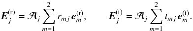 (A.1)As shown in
Paper I, the dimensionless emissivities for the two orthogonal linear polarizations are
Jj = 1 − Rj,
where
(A.1)As shown in
Paper I, the dimensionless emissivities for the two orthogonal linear polarizations are
Jj = 1 − Rj,
where  (A.2)The reflected field
amplitudes
r11,r12,r21,
and r22 were calculated in Paper I using an eighth-order
polynomial in the refraction index nj to
determine the properties of the transmitted modes. The transmitted wave can be described
by two normal modes, thus, most of the roots obtained from that polynomial represent
unphysical solutions to the equations. The conditions to identify the correct roots were
derived in Appendix B of Paper I, with the requirements that the corresponding
reflectivities satisfy
(A.2)The reflected field
amplitudes
r11,r12,r21,
and r22 were calculated in Paper I using an eighth-order
polynomial in the refraction index nj to
determine the properties of the transmitted modes. The transmitted wave can be described
by two normal modes, thus, most of the roots obtained from that polynomial represent
unphysical solutions to the equations. The conditions to identify the correct roots were
derived in Appendix B of Paper I, with the requirements that the corresponding
reflectivities satisfy  and that the function R(E) be continuous. However, for
some values of the model parameters, the unphysical roots can satisfy the physical
constraints on the solution.
and that the function R(E) be continuous. However, for
some values of the model parameters, the unphysical roots can satisfy the physical
constraints on the solution.
Here we propose an improved method, based on a fourth-order polynomial, which allows for easy elimination of the unphysical roots.
A.1. Transmitted modes
A significant simplification of the equations describing the transmitted mode
properties can be obtained by writing the transmitted wave vector as ![Mathematical equation: \appendix \setcounter{section}{1} \begin{eqnarray} \label{eq:wavevec} \bm{n}_j = \frac{c}{\omega}\bm{k}_j & = n_j \left[\sin\theta_j\left(\cos\varphi\,\hat{\vec{x}} + \sin\varphi\,\hat{\vec{y}}\right) + \cos\theta_j\,\hat{\vec{z}}\right] \nonumber\\ & = \sin\theta_k\left(\cos\varphi\,\hat{\vec{x}} +\sin\varphi\,\hat{\vec{y}}\right) + n_{z,j}\,\hat{\vec{z}}, \end{eqnarray}](/articles/aa/full_html/2012/10/aa19747-12/aa19747-12-eq251.png) (A.3)where
(A.3)where
 ,
,
 ,
,
 are unit vectors along the x, y, z
axes, respectively, and the quantities
cosθj,
sinθj are complex numbers satisfying
the condition:
cos2θj + sin2θj = 1
(cf. Appendix B of Paper I). The second equality in Eq. (A.3) follows from Snell’s Law,
njsinθj = sinθk,
and the definition
nz,j ≡ njcosθj.
are unit vectors along the x, y, z
axes, respectively, and the quantities
cosθj,
sinθj are complex numbers satisfying
the condition:
cos2θj + sin2θj = 1
(cf. Appendix B of Paper I). The second equality in Eq. (A.3) follows from Snell’s Law,
njsinθj = sinθk,
and the definition
nz,j ≡ njcosθj.
From Maxwell’s equations for the transmitted modes, 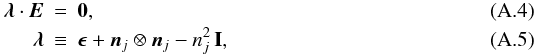 where
ϵ is the dielectric tensor of the medium (see Eq. (13)
of Paper I), I is the unit tensor, and
E is the electric field vector. If we note that
where
ϵ is the dielectric tensor of the medium (see Eq. (13)
of Paper I), I is the unit tensor, and
E is the electric field vector. If we note that
 , and apply
the condition detλ = 0 to obtain a nontrivial solution to
Eq. (A.4), the result is a
fourth-order polynomial in nz,j:
, and apply
the condition detλ = 0 to obtain a nontrivial solution to
Eq. (A.4), the result is a
fourth-order polynomial in nz,j:
 where
the coefficients have the values:
where
the coefficients have the values:  The
fourth order polynomial defined by Eqs. (A.6)–(A.21) has much better
numerical properties than the eighth-order polynomial described by Eq. (A.4) of Paper I.
We find that a stable, efficient method for solving Eq. (A.6) can be obtained by defining the matrix
The
fourth order polynomial defined by Eqs. (A.6)–(A.21) has much better
numerical properties than the eighth-order polynomial described by Eq. (A.4) of Paper I.
We find that a stable, efficient method for solving Eq. (A.6) can be obtained by defining the matrix
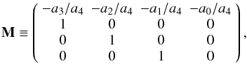 (A.22)and noting that the
eigenvalues of M are equal to the roots of Eq. (A.6). We use the ZGEEV subroutine of the
LAPACK library (Anderson et al. 1999) to compute
the eigenvalues of M. Of the resulting four roots, only two
correspond to physical solutions for the transmitted waves. To identify the correct
roots, we write the spatial variation of the transmitted electric field as
Ej (r) ∝ exp(iω nj·r/c).
The amplitude of the electric field must decay in the transmitted wave region, leading
to the condition:
(A.22)and noting that the
eigenvalues of M are equal to the roots of Eq. (A.6). We use the ZGEEV subroutine of the
LAPACK library (Anderson et al. 1999) to compute
the eigenvalues of M. Of the resulting four roots, only two
correspond to physical solutions for the transmitted waves. To identify the correct
roots, we write the spatial variation of the transmitted electric field as
Ej (r) ∝ exp(iω nj·r/c).
The amplitude of the electric field must decay in the transmitted wave region, leading
to the condition:  (A.23)At all
energies and angles for the range of magnetic fields
B = 1012−1015 G, condition (A.23) identifies two physical solutions to
Eq. (A.6). Using these values for
nj , we write the polarization vectors
for the transmitted wave as
(A.23)At all
energies and angles for the range of magnetic fields
B = 1012−1015 G, condition (A.23) identifies two physical solutions to
Eq. (A.6). Using these values for
nj , we write the polarization vectors
for the transmitted wave as 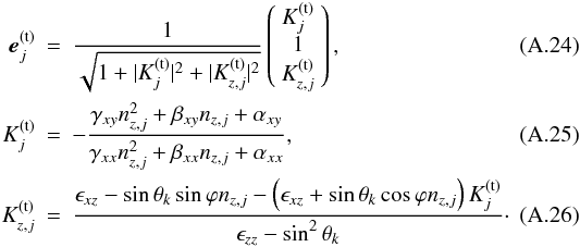
A.2. Reflectivity calculation
Once the quantities nj and
 are
known, the reflectivity of the medium can be calculated using the boundary conditions
for Maxwell’s equations at the condensed matter surface:
are
known, the reflectivity of the medium can be calculated using the boundary conditions
for Maxwell’s equations at the condensed matter surface:  where
ΔE ≡ E(i) + E(r) − E(t)
and
ΔB ≡ B(i) + B(r) − B(t)
are the differences between the fields above (incident and reflected) and below
(transmitted) the condensed surface. For the detailed forms of the fields, see Sect. 3.1
of Paper I. Writing out the components of (A.27) and (A.28) for the two
orthogonal linear polarizations of the incident wave yields a system of equations for
the amplitudes of the reflected and transmitted modes, analogous to Eq. (A.6) of
Paper I. This set of equations can be solved as two independent linear systems with
complex coefficients, such that
where
ΔE ≡ E(i) + E(r) − E(t)
and
ΔB ≡ B(i) + B(r) − B(t)
are the differences between the fields above (incident and reflected) and below
(transmitted) the condensed surface. For the detailed forms of the fields, see Sect. 3.1
of Paper I. Writing out the components of (A.27) and (A.28) for the two
orthogonal linear polarizations of the incident wave yields a system of equations for
the amplitudes of the reflected and transmitted modes, analogous to Eq. (A.6) of
Paper I. This set of equations can be solved as two independent linear systems with
complex coefficients, such that
 (A.29)where
 and
and

 We solve the complex
systems using the ZGESV subroutine of the LAPACK library (Anderson et al. 1999).
We solve the complex
systems using the ZGESV subroutine of the LAPACK library (Anderson et al. 1999).
The corrected results for the case of a magnetized iron surface (to be compared with Paper I) are presented in Sect. 2.2.3.
Appendix B: Approximations for reflectivities at the bottom of a thin atmosphere
B.1. Reflectivities of the normal modes in terms of rmj
In general, the interface between the thin atmosphere and magnetic condensed surface has reflection and transmission properties that are different from those of the condensed surface in vacuum. Therefore, a separate calculation of the reflectivity coefficients rmj is needed for every set of atmosphere parameters. However, assuming that the atmosphere is sufficiently rarefied, we may approximately replace these coefficients by those in vacuum. Under these conditions, the plane waves in the atmosphere are almost transverse, so we can approximately set Kz,M → 0 in Eq. (4). Then each incident and reflected wave can be expanded over the linear polarization vectors e1 and e2 that have been employed in the reflectivity calculation.
For the incident (i) and reflected (r) beams, we define orthonormal vectors
 ,
,
 , and
, and
 , where
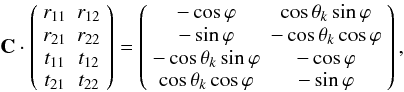
 denotes the unit vector along k. In the notations of
Fig. 1,
denotes the unit vector along k. In the notations of
Fig. 1, 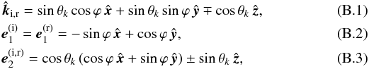 where
the upper and lower signs in ∓ cosθk are
for the incident and reflected waves, respectively. The coordinates in which Eq. (4) is written are
(x′,y′,z′)
(Fig. 1), defined according to relations
where
the upper and lower signs in ∓ cosθk are
for the incident and reflected waves, respectively. The coordinates in which Eq. (4) is written are
(x′,y′,z′)
(Fig. 1), defined according to relations
 and
and
 .
.
The electric field of the incoming ray with unit amplitude and polarization
M′ (M′ = X or
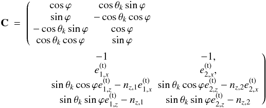
M′ = O) can be written as 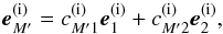 (B.4)where
 .
According to Eqs. (A.1) and (B.4), the reflected field is
.
According to Eqs. (A.1) and (B.4), the reflected field is
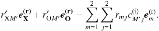 (B.5)The amplitudes
 and
and
 of the
reflected-field components in the X- and O-modes, respectively, are given by the
solution of the linear system
of the
reflected-field components in the X- and O-modes, respectively, are given by the
solution of the linear system 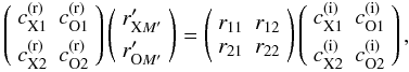 (B.6)where
 .
Since the incident X- and O-modes are incoherent, the normal mode reflectivities in
Eqs. (29) and (30) are
.
Since the incident X- and O-modes are incoherent, the normal mode reflectivities in
Eqs. (29) and (30) are
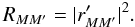 (B.7)According to
Eq. (4),
(B.7)According to
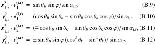
Eq. (4), 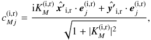 (B.8)where
 . The explicit expressions
for the scalar products in Eq. (B.8) are
. The explicit expressions
for the scalar products in Eq. (B.8) are
 Caution
should be used when employing approximations for
rmj in Eq. (B.6) if one of the normal modes is almost
completely reflected, that is,
RMM′ ≈ 1.
Such a situation occurs for the X-mode at
Eci < E < EC,
if both k and B are close to
normal (see Paper I). In this case the fit error may exceed
(1 − RXX) and result in
RXX > 1, which is unphysical. In
particular, the fitting formulae presented below may occasionally give
RXX a few percent above 1 at very small
θB and
θk. In such instances one should
truncate the mode-specific reflectivities, recovered from the fit, so as to fulfill the
general condition
0 < RMM′ < 1.
Caution
should be used when employing approximations for
rmj in Eq. (B.6) if one of the normal modes is almost
completely reflected, that is,
RMM′ ≈ 1.
Such a situation occurs for the X-mode at
Eci < E < EC,
if both k and B are close to
normal (see Paper I). In this case the fit error may exceed
(1 − RXX) and result in
RXX > 1, which is unphysical. In
particular, the fitting formulae presented below may occasionally give
RXX a few percent above 1 at very small
θB and
θk. In such instances one should
truncate the mode-specific reflectivities, recovered from the fit, so as to fulfill the
general condition
0 < RMM′ < 1.
B.2. Approximations for rmj
For calculating
RMM′
according to Sect. B.1, we use an analytic model
of the complex reflectivity coefficients
rmj, which agrees with the approximations
derived in Sect. 2.3 and roughly reproduces the
computed dependences of
rmj = |rmj|exp(iφmj)
on E for many characteristic geometry settings. For the squared moduli
we use the following expressions: 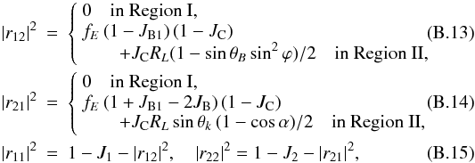 and
and
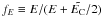 . The functions
J1, J2,
JB, JC,
JB1, and RL
are defined in Sect. 2.3. In the case of the
free-ions model, small accidental discontinuities at the boundary of Region I are
eliminated by truncating |r11|2 and
|r22|2 from above by their values at
E = Eci. Our approximations for the
complex phases are
. The functions
J1, J2,
JB, JC,
JB1, and RL
are defined in Sect. 2.3. In the case of the
free-ions model, small accidental discontinuities at the boundary of Region I are
eliminated by truncating |r11|2 and
|r22|2 from above by their values at
E = Eci. Our approximations for the
complex phases are 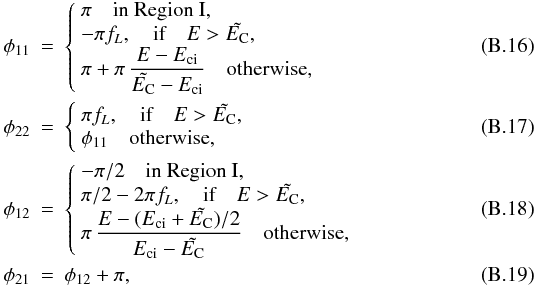 where
where
![Mathematical equation: \begin{equation*} f_L = \left[1+\exp\left( 5\, \frac{E_L-E}{E_L-\tilde\EC} \right)\right]^{-1}\cdot \end{equation*}](/articles/aa/full_html/2012/10/aa19747-12/aa19747-12-eq326.png)
All Figures
|
Fig. 1 Illustration of notations. The z axis is chosen perpendicular to
the surface, and the (xz) plane is chosen parallel to the
magnetic field lines, which make an
angle θB with the normal to the
surface. The direction of the reflected beam with wave vector
kr is determined by the polar
angle θk and the azimuthal
angle ϕ, and αr is the angle
between the reflected beam and the field lines. Thick solid lines show the
reflected beam and magnetic field directions, thin solid lines illustrate the
coordinates, and dashed lines show the incident photon wave vector
ki and its quadrant. The lines marked
|
| In the text | |
|
Fig. 2 Dimensionless emissivity J = 1 − R as a function of photon energy E for a condensed Fe surface with B = 1013 G and T = 106 K. The top panel shows several cases with varying θB and fixed θk = π/4, ϕ = π/4. The bottom panel shows several cases with varying ϕ and fixed θk = π/4, θB = π/4. These plots should be compared with Figs. 5 and 6 of Paper I. |
| In the text | |
|
Fig. 3 Dimensionless emissivity J = 1 − R as a function of photon energy E for condensed Fe surface at B = 1013 G (top panel), B = 1012 G and 1014 G (bottom panel), with magnetic field lines normal to the surface, for two angles of incidence θk = 0 and θk = π/4, as marked near the curves. Solid lines show our numerical results, and dashed lines demonstrate the fit. For comparison, dotted lines reproduce the simplified approximation used in Paper II. |
| In the text | |
|
Fig. 4 Dimensionless emissivity J = 1 − R as a function of photon energy E for a condensed Fe surface with inclined magnetic field (B = 1013 G, θB = π/4) and inclined incidence of radiation (θk = π/4 and four values of ϕ listed in the figure). Solid lines show our numerical results for the model of free ions at T = 106 K, and short-dashed lines demonstrate the fit. For comparison, the dotted line reproduces our numerical results for ϕ = π/2 and T = 3 × 10⁵ K. |
| In the text | |
|
Fig. 5 Same as in Fig. 4, but for B = 1014 G and two values of ϕ. For comparison, the dotted and long-dashed lines reproduce our numerical results and analytic approximation, respectively, for the model of fixed ions. |
| In the text | |
|
Fig. 6 Dimensionless emissivity for the linear polarization e1, J1 = 1 − R1, as a function of photon energy E for condensed Fe surface at different magnetic field strengths and geometric settings. Top panel: magnetic field B = 1013 G is normal to the surface, and angles of radiation incidence are θk = 0, π/6, π/4, and π/3. Bottom panel: B = 1013.5 G, magnetic field lines and the photon beam are both inclined at θB = θk = π/4, and the azimuthal angle takes values ϕ = 0, π/4, and π/2. Solid lines show the numerical results, and dashed lines demonstrate the fit. |
| In the text | |
|
Fig. 7 Degree of linear polarization Plin (Eq. (28)) as a function of photon energy E for condensed Fe surface. The values of B, directions of the field and the wave vector, and line types are same as in Fig. 6. |
| In the text | |
|
Fig. 8 Emergent spectra (top panel) and temperature structures (bottom panel) for the fiducial model atmosphere (solid curve) and for model atmospheres that are calculated using the fixed-ions approximation for the reflectivity calculations (dashed curves), and the inner boundary condition from Paper II (dotted curves). In the top panel the diluted blackbody spectrum that fits the high-energy part of the fiducial model spectrum is also shown (dash-dotted curve). |
| In the text | |
|
Fig. 9 Top panel: dimensionless emissivities for coefficients of reflection RXX (dashed curve), RXO (dotted curve), ROX (dash-dot-dotted curve), and ROO (dash-dotted curve). The quantities are calculated at the bottom of the fiducial model atmosphere for the angle between the radiation propagation and magnetic field, θk = 10°, together with the total dimensionless emissivity (solid curve). Bottom panel: dimensionless outward specific intensities (inner boundary condition) at the bottom of the fiducial model atmosphere for the X-mode (solid curve) and O-mode (dashed curve). For comparison, the dotted curve shows the same for the X-mode, calculated using the inner boundary condition from Paper II (in this case the dimensionless specific intensity of the O-mode equals 0.5). |
| In the text | |
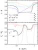 |
Fig. 10 The same as in Fig. 9, but for θk = 60°. |
| In the text | |
|
Fig. 11 Top panel: total emergent spectrum of the fiducial model (solid curve), together with emergent spectra in the X-mode (dashed curve) and in the O-mode (dash-dotted curve). The blackbody spectrum with T = Teff is also shown (dotted curve). Bottom panel: emergent specific intensities of the fiducial model for six angles θ. |
| In the text | |
|
Fig. 12 Comparison of emergent spectra (top panel) and temperature structures (bottom panel) of the fiducial model (solid curves) with the semi-infinite model atmosphere (dashed curves) and with the thinner (Σ = 1 g cm-2) model atmosphere (dotted curves), but with the same magnetic field. |
| In the text | |
|
Fig. 13 Comparison of emergent spectra (top panel) and temperature structures (bottom panel) of the fiducial model (solid curves) and the model atmosphere with different magnetic field (B = 1014 G), but with the same surface density (dashed curves). |
| In the text | |
Current usage metrics show cumulative count of Article Views (full-text article views including HTML views, PDF and ePub downloads, according to the available data) and Abstracts Views on Vision4Press platform.
Data correspond to usage on the plateform after 2015. The current usage metrics is available 48-96 hours after online publication and is updated daily on week days.
Initial download of the metrics may take a while.