| Issue |
A&A
Volume 546, October 2012
|
|
|---|---|---|
| Article Number | A72 | |
| Number of page(s) | 51 | |
| Section | Catalogs and data | |
| DOI | https://doi.org/10.1051/0004-6361/201219199 | |
| Published online | 08 October 2012 | |
Do Slivan states exist in the Flora family?
I. Photometric survey of the Flora region⋆
1 Astronomical Observatory Institute,
Faculty of Physics, Adam Mickiewicz University, Słoneczna 36, 60-286 Poznań, Poland
e-mail: This email address is being protected from spambots. You need JavaScript enabled to view it.
2 Institut de Mécanique Céleste et
Calcul des Éphémérides, Observatoire de Paris, 77 Av. Denfert Rochereau, 75014
Paris,
France
3 Institute of Astronomy, Bulgarian
Academy of Sciences Tsarigradsko Chausse 72, 1784
Sofia,
Bulgaria
4 Faculty of Natural Sciences, Cyril
and Methodius University Skopje,
Macedonia
5 Institute of Astronomy, Karazin
National University, Kharkov, Ukraine
6 Astrophysics Division, Institute of
Physics, Jan Kochanowski University, Świetokrzyska 15, 25-406
Kielce,
Poland
7 San Pedro de Atacama
Observatory, Chile
8 Observatoire de Paris,
5 place Jules Janssen,
92195
Meudon,
France
9 Geneva Observatory,
1290
Sauverny,
Switzerland
10 Institut de Recherche en
Astrophysique et Planétologie (IRAP), Université de Toulouse,
9 avenue du colonel Roche,
31028
Toulouse Cedex 4,
France
11 Observatoire de
Haute-Provence, 04870 Saint Michel
l’ Observatoire,
France
12 Observatoire des
Engarouines, 84570
Mallemort-du-Comtat,
France
13 Stazzione Astronomica di
Sozzago, 28060
Sozzago,
Italy
14 Le Cres Observatory,
Rue des Écoles 2, 34920
Le Cres,
France
15 Bedoin Observatory,
Avignon,
France
16 Department of Physics, PO Box 64,
00014 University of Helsinki, Finland
17 Nordic Optical Telescope, Apartado
474, 38700 Santa Cruz de La Palma, Santa Cruz de Tenerife, Spain
Received:
27
March
2012
Accepted:
23
June
2012
Abstract
Context. Recent studies have uncovered evidence that the statistical properties of asteroids’ physical parameters are a fundamental source of information on the physics of their collisions and evolution. The analysis of the spin rates and spin vector distributions helps us to understand the role of various known and new effects. The alignment of spin vectors and the correlation of spin rates are for the first time observed for ten members of the Koronis family. These unexpected non-random orientations of the spin axes and correlations of the spin rates, now known as Slivan states are interpreted in terms of a YORP effect and spin-orbit resonances.
Aims. To study non-gravitational-effects, there appears to be a need for new observational campaigns devoted to determining the physical parameters of the asteroid families.
Methods. We analysed the photometric observations of the asteroids, which are the most efficient method of studying asteroid physical parameters.
Results. We report the results of a ten-year long observational survey of the light variations of objects in the Flora region. We present 544 individual lightcurves of 55 objects obtained at various observing geometries. These lightcurves yield new or refined synodic periods for 32 asteroids and confirm period determinations for 23 objects in our sample. To improve the statistics of the Flora family objects, we add to our dataset 91 objects with reliably determined periods. The distribution of rotation rates for the Flora family is non-Maxwellian at a confidence level of 94% and different from those of the Koronis and the Hungaria families. It seems to be consistent with the long-term influence of the YORP effect, although it is also indicative of a younger age for the Flora family compared to both the Koronis and the Hungaria families.
Conclusions. Our new data is a foundation for the spin vector and shape determinations that will be the objectives of the second paper of the series. We search for spin vector and spin periods correlations in order to determine whether Slivan states exist in the Flora family.
Key words: techniques: photometric / minor planets, asteroids: general
Photometric data is available in electronic form at the CDS via anonymous ftp to cdsarc.u-strasbg.fr (130.79.128.5) or via http://cdsarc.u-strasbg.fr/viz-bin/qcat?J/A+A/546/A72
© ESO, 2012
1. Introduction
The number of known spin vectors of the main belt and near-Earth asteroids is regularly growing with the inclusion of new objects as well as the updating of data for known cases with the arrival of new observations and improved techniques. All of the asteroid spin-vector determinations published in the literature are available at the Poznan Astronomical Observatory website1. Up to now, this dataset includes data for about 250 objects although, only 170 have reasonably reliable determinations. For further discussion, we refer to both Kryszczynska et al. (2007), and references therein, and Paolicchi & Kryszczynska (2012).
Recent studies have provided evidence that the statistical properties of asteroid physical parameters are a fundamental source of information about the physics of their collisions and evolution. There are probably several different mechanisms shaping the distribution of spin-rate and spin-vector orientations of small MBAs and NEAs, leading us to expect that the distributions may be non-Maxwellian or even bi-modal. The analysis of the spin rates and spin vector distributions helps us to understand the role of various known and new effects.
Studies of NEA spin vectors, which are mostly smaller than D < 10 km, were reported by La Spina et al. (2004) to have a strong and statistically significant excess of retrograde rotators. This result is consistent with theoretical expectations for the Yarkovsky effect, which is assumed to be responsible for injecting main belt asteroids into resonant regions.
The alignment of asteroid spin vectors and the correlation of spin rates were for the first time observed for ten members of the Koronis family (Slivan 2002; Slivan et al. 2003). These unexpected nonrandom orientations of spin axes and corelation of spin rates, now known as Slivan states, were explained by Vokrouhlicky et al. (2003) in terms of the YORP effect and spin-orbit resonaces. They suggested that over the past few Gyr the YORP effect might have been more efficient than collisions in changing the spin rates and obliquities of main belt asteroids with diameters D < 40 km. Additional studies of the Koronis family asteroids (Vokrouhlicky et al. 2006; Slivan et al. 2009) confirmed previously found clustering, although one stray object has also been found. The number of objects with known spin vector parameters within Koronis family is now 15.
Vokrouhlicky et al. (2003) investigated whether small asteroids in the other main belt regions, may also be trapped in Slivan states. They concluded that Slivan states may be found for low inclination asteroids in the outer main belt. A more complex spin-vector evolutionary path was obtained for inner main-belt asteroids. They also suggested making a careful comparison between numerical results and observations.
An observing campaign targeting small bodies in the outer main belt would require continuous access to the one-metre class or larger telescopes with efficient CCD cameras. Because of the lack of such dedicated instruments, we decided to concentrate our observing campaign on small bodies in the inner main belt, namely the Flora region. The location of this region makes its members available for photometric observations using relatively small telescopes. Thus, we were able to reach small objects, of diameters smaller than 30 km, which are sensitive to the influence of both Yarkovsky and YORP effects. The Flora family has more than 500 members and is unusually dispersed across proper eccentricity and inclination. It is intersected by several mean-motion resonances with Mars and Jupiter. Zappala et al. (1990, 1995) and Bendjoya (1993) used two different methods: hierarchical clustering (HCM) and wavelet analysis (WAM) of classification asteroids into families. Both methods are in good agreement in the resulting family classifications. The Flora dynamical family is the biggest in their analysis and has several denser groupings, which is in good accordance with the commonly suggested multi-collisional-event origin of this family. Most of the objects defined as the Flora family by HCM and/or WAM are S type and only two of them 8 Flora and 43 Ariadne have diameters larger than 30 km.
Mothe-Diniz et al. (2005) reanalysed the structure of asteroid families using visible spectroscopy. Their results indicate that most of the families are quite homogenous taxonomicaly and mineralogically and probably originated from homogenous parent bodies. Using the HCM mathod, Mothe-Diniz et al. (2005) divided the Flora region into Baptistina family objects plus several small clumps. However, the division into clumps and their size depends on the adopted cutoff parameter. Eventually, clumps will merge together but at the same time they will merge with Vesta family. Unfortunately only eight members of the Baptistina family have known spectra and six of them are different than S type. Taking into account groupings only, the Belgica clump has more than three members with known spectra and all the objects are of S type.
The latest family identification was done by Nesvorny (2010). Using HCM method and proper elements for 293 368 asteroids, he obtained 55 families. In this classification, the Flora family contains 10 437 members and belongs to the three most-abundant families. It is surprising that the large asteroid 9 Metis, whose diameter is even larger than that of 8 Flora, as well as 113 Amalthea and 376 Geometria, now belongs to this family. The largest objects, unaffected by the nongravitational effects, are not taken into account in this study.
Our observing campaign was devoted to all objects smaller than 30 km classified by HCM and/or WAM as Flora family members. Objects identified as binary systems, namely 809 Lundia, 939 Isberga, 1089 Tama, 1338 Duponta, 1830 Pogson, 1857 Parchomenko, 2121 Sevastopol, 2691 Sersic, 2815 Soma, 2478 Tokai, 3073 Kursk, and 3749 Balam, were not taken into account in this study.
2. Observations and data reduction
Because many of the periods of rotation for the Flora family asteroids have been reported by amateurs only, or have been based on low quality lightcurves, we decided to observe as many objects as possible. Our regular photometric observations of the Flora family asteroids started in 2002. However, some lightcurves were obtained by us before this year. In this paper, we report 544 individual lightcurves of 55 asteroids observed at fifteen observatories: Borowiec (Poland), Pic du Midi (France), National Astronomical Observatory, Rozhen (Bulgaria), Kharkov (Ukraine), South African Astronomical Observatory (South Africa), San Pedro de Atacama (Chile), Pico dos Dias (Brazil), Kielce (Poland), Poznan Observatory (Poland), Les Engarouines (France), Observatorio del Roque de los Muchatos (Spain), Haute-Provence Observatory (France), Le Cres (France), Bedoin Observatory (France), and Stazzione Astronomica di Sozzago (Italy). We note that we were limited only by the brightness of the observed objects and weather conditions.
Observations in Borowiec were carried out with a 0.4 m F/4.5 Newton reflector equipped with KAF400 and (since September 2009) KAF402ME CCD cameras and a set of Bessel BVRI and clear (C) filters. Details of the Borowiec system are described in Michalowski et al. (2004). Some of the lightcurves from Borowiec were obtained using Poznan Spectroscopic Telescope (PST), which consists of parallel twin 0.5 m f/4.5 Newton telescopes on a single parallactic fork mount. Two KAF400 CCD cameras were mounted at the primary focus of both mirrors. Details of this telescope are described in Baranowski et al. (2007).
Lightcurves observed at Pic du Midi were obtained using the 1.05 m Cassegrain telescope equipped with THX 7863 CCD camera and R, DH, or L filters. Since October 2010, the Andor iKon-L 2048 × 2048 pixels CCD camera was used. A standard reduction for bias and flatfield of the Pic du Midi observations were done using Astrol package developed at IMCCE in Paris and Starlink package2. Observations from Borowiec were reduced for bias, dark current and flatfield using the Starlink package. The aperture photometry of Borowiec and Pic du Midi frames was carried out with the PHOTOM programme included in the Starlink package.
Observations at the National Astronomical Observatory at Rozhen were carried out with the 50/70 cm f/3.44 Schmidt telescope equipped with a KAF1602E 1530 × 1020 pixels CCD camera and Bessel VR filters, and with a 2 m RCC f/8 telescope equipped with a Photometrics CE200A 522 × 512 pixels CCD camera and R filter. For the data reduction and aperture photometry, IDL software was used.
Kharkov data were collected at the Grakovo Observing Station with the 0.7 m reflector. equipped with a IMG 1024S CCD camera and Johnson UBVRI filters. Data reduction was carried out using ASTPHOT software developed by Stefano Mottola (Mottola et al. 1995; Erikson et al. 2000).
Observations at South African Astronomical Observatory were done with the 0.76 m Cassegrain telescope and WRT1 420 × 289 pixel CCD camera in 2008 and 2009, and KAF1603ME 1530 × 1020 pixel CCD camera in 2010. Kielce observations were done using the 0.35 m Schmidt-Cassegrain reflector with the SBIG ST7XE CCD camera (KAF0401E chip) and C or V Bessel filter.
Observations at Pico dos Dias were carried out with the 0.6 m f/12.5 Zeiss telescope equipped with a EEV 400 × 290 pixels CCD, mounted at the Cassegrain focus and R filter.
San Pedro de Atacama data were collected with the CAO 0.4 m F/7.7 reflector and KAF1603ME, 1530 × 1020 pixel CCD camera clear filter.
Lightcurves from Observatorio del Roque de los Muchachos were produced using the 2.56 m Nordic Optical Telescope (NOT) and ALFOSC (The Andalucia Faint Object Spectrograph and Camera) with back-side illuminated EEV CCD camera and R filter.
Poznan Observatory lightcurves were obtained with a 0.7 m robotic Planewave CDK700 f/6.6 reflector, during its commissioning stage, equipped with Andor iXon back-side illuminated CCD and clear filter.
Data from SAAO, Kielce, Pico dos Dias, San Pedro de Atacama, Les Engarouines, NOT and Poznan were reduced for bias, dark current (not required for Andor cameras) and flatfield using Starlink package. Aperture photometry of all of the above mentioned data was carried out with PHOTOM programme included in Starlink package.
Details of the instruments used in Haute-Provence Observatory (France), Les Engarouines (France), Stazzione Astronomica di Sozzago (Italy), Le Cres Observatory (France), and Bedoin Observatory (France) can be found at the website of Geneva Observatory maintained by Raoul Behrend3.
Most of the observed lightcurves have a scatter of points at a level of 0.01 mag with respect to the fitted fourth-order Fourier harmonics. Systematic effects caused by changes in the viewing geometry influence the shape of the observed lightcurves and the obtained synodic periods. Period determination was done using the procedure described by Magnusson & Lagerkvist (1990). In each case, the uncertainty in the period was determined by changing the value of the period to find the worst tolerable fit of the composite lightcurve. Because of this, the reported uncertainties of the periods are maximal errors rather than standard deviations. We note that the synodic period for a given asteroid may vary by typically up to 0.0005 h between apparitions. Because of that, making efforts to derive synodic periods with higher accuracy is of little importance. The reported lightcurves will be a good foundation for future spin-vector and shape determinations, which will appear in the second paper of the series. A description of individual objects as well as composite lightcurves and aspect data are available in Appendix A.
3. Properties of the the Flora asteroids
Observations of 55 individual Flora family objects resulted in 544 lightcurves. They yielded new or refined synodic periods for 32 objects and confirmed period determinations for 23 asteroids. To improve the statistics of the Flora family asteroids and avoid eventual observational bias, we added to our dataset 91 objects up to number 4150 having published secure nonambiguous solutions for their periods based on the full lightcurve coverage (reliability/quality code ≧ 3, see Lagerkvist et al. 1989, or International Astronomical Union (IAU) Minor Planet Lightcurve Parameters). We searched the Asteroid Lightcurve Database4 released on August 2011. Moreover, we checked the original sources where period determinations were reported. We also searched rotation curves of asteroids available at the website maintained by Raoul Behrend5.
This process provided a total sample of 146 Flora asteroids with known synodic rotation-periods. Table 1 summarizes the physical data of our sample: diameters (D [km]), absolute magnitudes (H [mag]), maximum amplitudes of the observed lightcurves (A [mag]), a geometric albedo (pv), the synodic period of rotation (P [h]), a frequency of rotation (f [1/d]), a taxonomic type, and classification to the family by HCM and WAM. Objects observed within this survey are marked in boldface. Most of the diameters and geometric albedos are taken from AcuA (Asteroid Catalog Using AKARI/IRC mid-infrared survey, Usui et al. 2011). They are marked with A. The other diameters are calculated from MPC absolute magnitudes and albedo using the standard formula 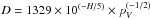 (Fowler & Chillemi 1992; Pravec & Harris 2007). Families in the main belt are quite homogenous taxonomically (Cellino et al. 2002; Mothe-Diniz et al.2005). Most of the objects identified as the Flora family are of taxonomic S-type. We calculated an average albedo for S-type objects from AcuA for 65 Flora family objects contained in Table 1. This average value of albedo of 0.25 is assumed for the other S-type asteroids and for objects with unknown taxonomic type. For three C-type objects (1523 Pieksamaki, 2093 Genichesk, 2283 Bunke) we assumed an albedo of 0.057. For D-type 827 Wolfiana we assumed an albedo of 0.04 and 0.15 for X-type 3533 Toyota. Taxonomic types given in Table 1 are taken from the collection of asteroid taxonomic classifications from various classification methods, collected from the literature (Neese 2010) and are indicated with 1. Types from the SDSS-based Asteroid Taxonomy (Hasselman et al. 2011) are marked with 2 and from Alvarez-Candal et al. (2006) are marked with 3. Maximum lightcurve amplitudes for objects not observed within this survey are taken from the Asteroid Lightcurve Database 4 version released on August 2011.
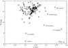 |
Fig. 1 Absolute magnitude H (mag) as a function of semimajor axis a (AU) for 146. Flora family asteroids. |
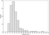 |
Fig. 2 Histogram of the diameters of the Flora family objects from our sample, the largest objects 8 Flora (138 km), 9 Metis (166 km), 43 Ariadne (59 km), and 113 Amalthea (46 km) are excluded. |
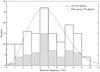 |
Fig. 3 Solid line – observed rotation-rate distribution for 142 objects of the Flora family. Asteroids observed within this campain are marked in grey. The dashed curve represents the Maxwellian distribution, for a mean squared frequency of 5.47 1/d, which is inconsistent with the sample at the 94% confidence level. The asteroids 8 Flora, 9 Metis, 43 Ariadne and 113 Amalthea are excluded. |
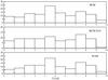 |
Fig. 4 Observed rotation-rate distribution for objects of the Flora family classified by different methods. 8 Flora, 9 Metis, 43 Ariadne, and 113 Amalthea are excluded. |
In the last three columns of Table 1, we present the membership to the family with specifications of the family identification technique: HCM – Zappala et al. (1995), WAM – Bendjoya (1993), Zappala et al. (1995), and HCM 2010 – Nesvorny (2010).
Only 8 Flora, 9 Metis, 43 Ariadne, and 113 Amalthea have diameters larger than 40 km. 9 Metis, 113 Amalthea, and 376 Geometria appear as Flora-family objects only in the latest family identification – HCM 2010. Figure 1 shows that these objects, especially 9 Metis and 113 Amalthea, as well as 376 Geometria, 428 Monachia, and 2853 Harvill are far from the main grouping of the family. A histogram of the diameters of the objects used in this study is presented in Fig. 2. The majority of the studied objects have diameters from 6 km to 14 km.
The observed rotation-rate distribution for 142 asteroids smaller than 35 km is presented in Fig. 3 (solid line). The grey columns represent the rotation-rate distribution for 55 objects observed within this study. The distribution is qualitatively similar to the statistics when extended to 142 objects. The only differences are visible for the fastest and the slowest rotators. We did not observe objects rotating faster than 9 cycles per day. For four very slow rotators observed by us, the dataset was insufficent to obtain a unique solution for their periods. From this reason these objects did not appear in the first bin of the histogram presented in Fig. 3. This also explains the discrepancy between the number of objects of our and the extended sample in the first bin of the histogram. These four objects however are less than 7% of our sample and are not of crucial importance.
The dashed curve represents the Maxwellian distribution for the mean squared spin frequency of 5.47 d-1. The Kolmogorov-Smirnov one sample test made with Mathematica confirms that the distribution of rotation rates in the Flora family is inconsistent with a Maxwellian distribution at a confidence level of 94%. We see an excess of fast and slow rotators and a peak around 4–5 rotations per day, which might still be connected with the original spin rate of the family parent body.
The observed rotational rate distribution does not depend on the classification method, Fig. 4. The asteroid sample for HCM 2010 is less abundant but the distribution is qualitatively similar. We also checked whether possible interlopers namely objects with other than a S taxonomic type, may influence the spin rate distribution. The result was negative.
Figure 5 presents the relation between the frequency of rotation and the diameter for 146 Flora family asteroids. All objects larger than 16 km rotate slower than five cycles per day. Objects smaller than 16 km have all possible frequencies. The only exception is the X-type asteroid 428 Monachia.
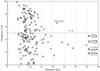 |
Fig. 5 Relation between frequency of rotation and diameter for 146 Flora family objects. All objects larger than 16 km rotate slower than 5 cycles per day. Smaller objects present all possible variety of frequencies. |
4. Discussion
A collisionaly evolved asteroid population should have a Maxwellian distribution of spin rates (Salo 1987). This behaviour is observed for objects with D > 40 km (Pravec et al. 2002 and references therein). The distribution of the spin rates of small asteroids (with 0.15 km < D < 10 km) is strongly non-Maxwellian with a significant excess of fast and slow rotators. The smallest main-belt/Mars-crossing asteroids with diameters 3 km < D < 15 km have a uniform distribution of frequencies from 1 d-1 to 9.5 d-1 and a strong excess of slow rotators for frequencies lower than 1 d-1, owing to the YORP effect (Pravec et al. 2008). Pravec et al. (2002) did not study in detail the transitional region where groups of large and small asteroids overlap. Some objects in this diameter range are members of the dynamical families.
The distribution of spin rates in the Flora family presented in Fig. 3 differs significantly from the distribution reported for the Koronis family by Slivan et al. (2008) and the Hungaria family by Warner et al. (2009b). Flora family asteroids do not have such a strong excess of slow rotators as the two other families. The dynamical evolution of the Flora family was studied by Nesvorny et al. (2002). They concluded that the age of the Flora family is significantly younger than 1 Gyr or even 0.5 Gyr. Cratering on 951 Gaspra suggests an even younger age of 200 Myr for the Flora family (Chapman 2002). The above-mentioned values are significantly younger than the age of the Koronis family 2–3 Gyr based on either the cratering of 243 Ida (Chapman 2002) or dynamical simulations (Vokrouhlicky et al. 2003 and references therein). The Hungaria dynamical family is younger than Koronis and its age is estimated to be about 0.5 Gyr (Warner et al. 2009b).
If we assumed that the spin rates are modified by nongravitational forces such as the YORP effect in the case of Flora clan, it would have had much less time to leave its fingerprint. The spin rate distribution confirms that Flora is younger than both the Koronis and Hungaria families.
In the following paper, we continue our study of the possible influence of the YORP effect on the spin axes of Flora family asteroids. We search for spin vector and spin period correlations to dermine whether Slivan States exist in the Flora family.
Physical data of the Flora family asteroids.
Acknowledgments
A.K. and M.P. thank Iwona Wytrzyszczak for her help with the Kolmogorov-Smirnov test. A.K. was supported by the Polish Grant N N203 382136, M.P. was supported by the Polish Grant N N203 387937, G.A. gratefully acknowledge observing grant support from the Institute of Astronomy and Rozhen National Astronomical Observatory, Bulgarian Academy of Sciences. V.A. was partially supported by a contract DO 02-85 between the Institute of Astronomy from Bulgarian Academy of Science and Bulgarian Ministry of Education, Youth, and Science. Observations of 4150 Starr and 1667 Pels were made with the Nordic Optical Telescope, operated on the island of La Palma jointly by Denmark, Finland, Iceland, Norway, and Sweden, in the Spanish Observatorio del Roque de los Muchachos of the Instituto de Astrofisica de Canarias. The work of TSR was carried out through the Gaia Research for European Astronomy Training (GREAT-ITN) network. He received funding from the European Union Seventh Framework Programme (FP7/2007-2013) under grant agreement No. 264895. This work is partially based on observations made at the South African Astronomical Observatory (SAAO). The reduction of most of the CCD data was performed with the CCLR STARLINK package.
References
- Almeida, R., Angeli, C. A., Duffard, R., & Lazzaro, D. 2004, A&A, 415, 403 [NASA ADS] [CrossRef] [EDP Sciences] [Google Scholar]
- Alvarez-Candal, A., Duffard, R., Lazzaro, D., & Mitchenko, T. 2006, A&A, 459, 969 [NASA ADS] [CrossRef] [EDP Sciences] [Google Scholar]
- Angeli, C. A., Guimares, T. A., Lazzaro, D., et al. 2001, AJ, 121, 2245 [NASA ADS] [CrossRef] [Google Scholar]
- Apostolovska, G., Ivanova, V., & Kostov, A. 2009, MP Bull., 36, 27 [Google Scholar]
- Baranowski, R., Smolec, R., Dimitrov, W., et al. 2009, MNRAS, 396, 2194 [NASA ADS] [CrossRef] [Google Scholar]
- Behrend, R., Bernasconi, L., Roy, R., et al. 2004, A&A, 446, 1177 [NASA ADS] [CrossRef] [EDP Sciences] [Google Scholar]
- Bendjoya, P. 1993, A&AS, 102, 25 [NASA ADS] [Google Scholar]
- Bennefeld, C., Aguilar, V., Cooper, T., et al. 2009, MP Bull., 36, 123 [Google Scholar]
- Binzel, R. P., & Mulholland, J. D. 1983, Icarus, 56, 519 [NASA ADS] [CrossRef] [Google Scholar]
- Binzel, R. P., Cochran, A. L., Barker, E. S., et al. 1987, Icarus, 71, 148 [NASA ADS] [CrossRef] [Google Scholar]
- Binzel, R. P., Gaffey, M. J., Thomas, P. C., et al. 1997, Icarus, 128, 95 [NASA ADS] [CrossRef] [Google Scholar]
- Birlan, M., Barucci, M. A., Angeli, C., et al. 1996, Planet. Space Sci., 44, 555 [NASA ADS] [CrossRef] [Google Scholar]
- Bottke, W. F., Vokrouhlicky, D., Rubincam, D. P., & Broz, D. P. 2002, in Asteroids III, eds. W. F. Bottke, A. Cellino, P. Paolicchi, & R. P. Binzel (Tucson: Univ. Arizona Press), 395 [Google Scholar]
- Bottke, W. F., Vokrouhlicky, D., Rubincam, D. P., & Nesvorny, D. 2006, Ann. Rev. Earth Planet. Sci., 34, 157 [Google Scholar]
- Bottke, W. F., Vokrouhlicky, D., & Nesvorny, D. 2007, Nature, 449, 48 [NASA ADS] [CrossRef] [Google Scholar]
- Brinsfield, J. W. 2008, MP Bull., 35, 179 [Google Scholar]
- Britt, D. T., & Consolmagno, G. J. 2004, 35th Lunar and Planetary Science Conference, League City, Texas, abst. 2108 [Google Scholar]
- Britt, D. T., Yeomans, D., Housen, K., & Consolmagno, G. J. 2002, in Asteroids III, eds. W. F. Bottke, A. Cellino, P. Paolicchi, & R. P. Binzel (Tucson: Univ. Arizona Press), 103 [Google Scholar]
- Buchheim, R. K. 2010, MP Bull., 37, 41 [Google Scholar]
- Carbo, L., Green, D., Khragh, K., et al. 2009, MP Bull., 36, 152 [Google Scholar]
- Carruba, V., Mitchenko, T. A., Roig, F., Ferraz-Mello, S., & Nesvorny, D. 2005, A&A, 441, 819 [NASA ADS] [CrossRef] [EDP Sciences] [Google Scholar]
- Carvano, J. M., & Lazzaro, D. 2010, MNRAS, 404, L31 [NASA ADS] [Google Scholar]
- Cellino, A., Pannunzio, R., Zappala, V., et al. 1985, A&A, 144, 355 [NASA ADS] [Google Scholar]
- Cellino, A., Buss, S.J., Doressoundiram, A., & D. Lazzaro, 2002, in Asteroids III, eds. W. F. Bottke, A. Cellino, P. Paolicchi, & R. P. Binzel (Tucson: Univ. Arizona Press), 633 [Google Scholar]
- Chapman, C. R. 2002, in Asteroids III, eds. W. F. Bottke, A. Cellino, P. Paolicchi, & R. P. Binzel (Tucson: Univ. Arizona Press), 315 [Google Scholar]
- Clark, M. 2004, MP Bull., 31, 15 [Google Scholar]
- Denchev, P., Shkodrov, V., & Ivanova, V. 2000, Planet. Space Sci., 48, 983 [NASA ADS] [CrossRef] [Google Scholar]
- Ditteon, R., & Hawkins, S. 2007, MP Bull., 34, 59 [Google Scholar]
- Di Martino, M. 1986, in Asteroids, Comets, Meteors II, eds. C.-I. Lagerkvist, B. A. Lindblad, M. Lundstedt, & H. Rickman, 81 [Google Scholar]
- Di Martino, M., Blanco, C., Riccioli, D., & de Sanctis, G. 1994a, Icarus, 107, 269 [NASA ADS] [CrossRef] [Google Scholar]
- Di Martino, M., Dotto, E., Barucci, M. A., et al. 1994b, Icarus, 109, 210 [NASA ADS] [CrossRef] [Google Scholar]
- Drummond, J. D., Fugate, R. Q., Christou, C., & Hege, E .K. 1998, Icarus, 132, 80 [NASA ADS] [CrossRef] [Google Scholar]
- Erikson, A., Mottola, S., Lagerros, J. S. V., et al. 2000, Icarus, 147, 487 [NASA ADS] [CrossRef] [Google Scholar]
- Fauerbach, M., Marks, S. A., & Lucas, M. P. 2008, MP Bull., 35, 44 [Google Scholar]
- Florczak, M., Lazzaro, D., & Duffard, R. 2002, Icarus, 159, 178 [NASA ADS] [CrossRef] [Google Scholar]
- Fowler, J. W., & Chillemi, J. R. 1992, in IRAS asteroid data processing, eds. E. F. Tedesco, G. J. Veeder, J. W. Fowler, & J. R. Chillemi, The IRAS Minor Planet Survey, Technical Report PL-TR-92-2049, Phillips Laboratory, Hanscom AF Base, MA [Google Scholar]
- Hamanowa, H., & Hamanowa, H. 2009, MP Bull., 36, 87 [Google Scholar]
- Hansen, A. T., Arentoft, T., & Lang, K. 1997, MP Bull., 24, 17 [Google Scholar]
- Hasselmann, P. H., Carvano, J. M., & Lazzaro, D. 2011, SDSS-based Asteroid Taxonomy V1.0, EAR-A-I0035-5-SDSSTAX-V1.0, NASA Planetary Data System [Google Scholar]
- Higgins, D., & Pilcher, F. 2009, MP Bull., 36, 143 [Google Scholar]
- Kaasalainen, M., Lamberg L., Lumme, K., & Bowell, T. 1992, A&A, 259, 318 [NASA ADS] [Google Scholar]
- Kryszczynska, A., Colas, F., Berthier, J., et al. 1996, Icarus, 124, 134 [NASA ADS] [CrossRef] [Google Scholar]
- Kryszczynska, A., La Spina, A., Paolicchi P., et al. 2007, Icarus, 192, 223 [NASA ADS] [CrossRef] [Google Scholar]
- Lagerkvist, C.-I. 1978, A&AS, 31, 361 [NASA ADS] [Google Scholar]
- Lagerkvist, C.-I. 1979, Icarus, 38, 106 [NASA ADS] [CrossRef] [Google Scholar]
- Lagerkvist, C.-I. Harris, A. W., & Zappala, V. 1989, in Asteroids II, eds. R. P. Binzel, T. Gehrels, & M. Mathews (The Univ. of Arizona Press), 1162 [Google Scholar]
- La Spina, A. Paolicchi, P., Kryszczynska, A., & Pravec P. 2004, Nature, 428, 400 [NASA ADS] [CrossRef] [PubMed] [Google Scholar]
- Lazar, S., Lazar, P., Cooney, W., & Wefel, K. 2001, MP Bull., 28, 33 [Google Scholar]
- Licchelli, D. 2006, MP Bull., 33, 105 [Google Scholar]
- Magnusson, P., & Lagerkvist, C.-I., 1990, A&AS, 86, 45 [NASA ADS] [Google Scholar]
- Majaess, D. J., Higgins, D., Molnar, L. A., et al. 2009, JRASC 103, 7 [NASA ADS] [Google Scholar]
- Menke, J. L. 2005, MP Bull., 32, 64 [Google Scholar]
- Michałowski, T., Colas, F., Kwiatkowski, T., et al. 2002, A&A, 396, 293 [NASA ADS] [CrossRef] [EDP Sciences] [Google Scholar]
- Michałowski, T., Kwiatkowski, T., Kaasalainen, M., et al. 2004a, A&A, 416, 353 [NASA ADS] [CrossRef] [EDP Sciences] [Google Scholar]
- Michałowski, T., Bartczak, P., Velichko, F. P., et al. 2004b, A&A, 423, 1159 [NASA ADS] [CrossRef] [EDP Sciences] [Google Scholar]
- Mothe-Diniz, T., Roig, F., & Carvano, J. M. 2005, Icarus, 174, 54 [NASA ADS] [CrossRef] [Google Scholar]
- Mottola, S., De Angelis, G., Di Martino, S., et al. 1995, Icarus, 117, 62 [NASA ADS] [CrossRef] [Google Scholar]
- Neese, C. 2010, Asteroid Taxonomy V6.0, EAR-A-5-DDR-TAXONOMY-V6.0, NASA Planetary Data System [Google Scholar]
- Nesvorny, D. 2010, Nesvorny HCM Asteroid Families V1.0, EAR-A-VARGBDET-5-NESVORNYFAM-V1.0, NASA Planetary Data System [Google Scholar]
- Nesvorny, D., Morbidelli A., Vokrouhlicky, D., et al. 2002, Icarus, 157, 155 [NASA ADS] [CrossRef] [Google Scholar]
- Oey, J. 2006, MP Bull. 33, 96 [Google Scholar]
- Oey, J., & Krajewski, R. 2008, MP Bull. 35, 47 [Google Scholar]
- Paolicchi, P., & Kryszczynska, A. 2012, Planet. Space Sci., in press [Google Scholar]
- Piironen, J., et al. 1998, A&AS, 128, 525 [NASA ADS] [CrossRef] [EDP Sciences] [Google Scholar]
- Pilcher, F., Binzel, R. P., & Tholen, D. J. 1985, MP Bull., 12, 10 [Google Scholar]
- Pravec, P., & Harris, A. W. 2007, Icarus, 190, 250 [CrossRef] [Google Scholar]
- Pravec., P., Harris, A. W., & Michalowski, T. 2002, in Asteroids III, eds. W. F. Bottke, A. Celino, P. Paolicchi, & R. P. Binzel (The Univ. of Arizona Press), 113 [Google Scholar]
- Pravec, P., Harris, A. W., Vokrouhlicky, D., et al. 2008, Icarus, 497 [Google Scholar]
- Pray, D., Galad, A., Gajdos, S., et al. 2006, MP Bull., 33, 92 [Google Scholar]
- Riccioli, D., Blanco, C., & Cigna, M. 2001, A&AS, 49, 657 [Google Scholar]
- Rubincam, D. P. 2000, Icarus, 148, 2 [NASA ADS] [CrossRef] [Google Scholar]
- Ruthroff, J. C. 2009, MP Bull. 36, 121 [Google Scholar]
- Salo, H. 1987, Icarus, 70, 37 [NASA ADS] [CrossRef] [Google Scholar]
- Schiller, Q., & Lacy, C. H. S. 2008, MP Bull. 35, 41 [Google Scholar]
- Slivan, S. M. 2002, Nature, 419, 49 [Google Scholar]
- Slivan, S. M., Binzel, R. P., Crespo da Sliva, L. D., et al. 2003, Icarus, 162, 285 [NASA ADS] [CrossRef] [Google Scholar]
- Slivan, S. M., Binzel, R. P., Boroumad, S. C., et al. 2008, Icarus, 195, 226 [NASA ADS] [CrossRef] [Google Scholar]
- Slivan, S. M., Binzel, R. P., Kaasalainen M., et al. 2009, Icarus, 200, 514 [NASA ADS] [CrossRef] [Google Scholar]
- Stephens, R. D. 2008, MP Bull. 35, 60 [Google Scholar]
- Taylor, R. C., Gehrels, T., & Capen, R. C. 1976, AJ, 81, 778 [NASA ADS] [CrossRef] [Google Scholar]
- Tedesco, E. F. 1979, Ph.D. Thesis, New Mexico State University [Google Scholar]
- Tedesco, E. F. 1989, in Asteroids II, eds. R. P. Binzel, T. Gehrels, & M. S. Matthews, 1090 [Google Scholar]
- Usui, F., Kuroda, D., Muller, T. G., et al. 2011, PASJ 63, 1117 [NASA ADS] [CrossRef] [Google Scholar]
- Vokrouhlicky, D., Nesvorny, D., & Bottke, W. F. 2003, Nature, 425, 147 [NASA ADS] [CrossRef] [PubMed] [Google Scholar]
- Vokrouhlicky, D., Broz, M., Michalowski, T., et al. 2006, Icarus, 180, 217 [NASA ADS] [CrossRef] [Google Scholar]
- Warner, B. 2000, MP Bull., 27, 21 [Google Scholar]
- Warner, B. 2002, MP Bull., 29, 74 [Google Scholar]
- Warner, B. 2008, MP Bull., 35, 67 [Google Scholar]
- Warner, B. 2009a, MP Bull., 36, 109 [Google Scholar]
- Warner, B. 2009b, MP Bull., 36, 172 [Google Scholar]
- Warner, B. 2010, MP Bull. 37, 57 [Google Scholar]
- Warner, B., Harris, A. W., & Pravec, P. 2009a, Icarus, 202, 134 [NASA ADS] [CrossRef] [Google Scholar]
- Warner, B., Harris, A. W., Vokrouhlicky, D., et al. 2009b, Icarus, 204, 172 [NASA ADS] [CrossRef] [Google Scholar]
- Wisniewski, W. Z. 1991, Icarus, 90, 117 [NASA ADS] [CrossRef] [Google Scholar]
- Wisniewski, W. Z., Michalowski, T., Harris, A. W., & MacMilan, R. S. 1997, Icarus, 126, 395 [NASA ADS] [CrossRef] [Google Scholar]
- Yang, X.-Y., Zhang, Y.-Y., & Li, X.-Q. 1965, Acta Astron. Sin., 13, 66 [Google Scholar]
- Zappala, V., Cellino, A., Farinella, P., & Knezevic, Z. 1990, AJ, 100, 2030 [NASA ADS] [CrossRef] [Google Scholar]
- Zappala, V., Bendjoya, P., Cellino, A., et al. 1995, Icarus, 116, 291 [NASA ADS] [CrossRef] [Google Scholar]
Appendix A: Description of the individual cases
Here we present in detail the results of our observing campaign. All the observed objects are fully described. Composite lightcurves are folded with periods determined and checked during this study. Aspect data for all of the observed lightcurves are available in Table A.1. Columns give dates of observations with respect to the middle of the lightcurve, asteroid distances to the Sun (r) and the Earth (Δ) in AU, phase angle (α), observer-centred ecliptic longitude (λ) and latitude (β) for J2000.0, and the observatory code (Obs).
A.1. 281 Lucretia
Taylor et al. (1976) reported photometric observations of Lucretia from 1969, 1972, and 1974. They obtatined a synodic period of 4.348 h and concluded that the spin axis of Lucretia is nearly perpendicular to the ecliptic.
We observed Lucretia on nine nights during four oppositions in 2003, 2006, 2008/2009, and 2011 in Borowiec and Rozhen. Our synodic period of 4.349 ± 0.001 h confirms Taylor’s et al. determination. All the lightcurves observed for this asteroid have similar amplitudes of 0.30–0.40 mag, implying that the spin vector has a high latitude. Our composite lightcurves are presented in Figs. A.1–A.4.
A.2. 291 Alice
The first preliminary model of 291 Alice published by Kryszczynska et al. (1996) was based on only six lightcurves from three oppositions in 1974 (Lagerkvist 1978), 1981 (Binzel & Mulholland 1983) and 1994 (Kryszczynska et al. 1996). Subseqent observations of this object from three nights in February 1996 were reported by Piironen et al. (1998). These data are rather sparse and no attempt to the asteroid modelling was made in that paper. All of the above-mentioned papers gave the same synodic period of 4.32 h for Alice. Oey (2006) observed Alice on three nights in 2006 and obtained a period of 4.313 h. Ruthroff (2009) observed Alice on four nights in 2009 and obtained a period of 4.32 h Single lightcurves from 2009 and 2010 available at6 have periods of 4.28 h and 4.30 h.
Our observations of Alice were done during four apparitions in 1999 (Fig. A.5), 2004 (Fig. A.6), 2007 (Fig. A.7), and 2009 (Fig. A.8) at Pic du Midi and Borowiec. We obtained ten new dense lightcurves at four different observing geometries. The improved value of synodic period of 4.316 ± 0.001 h closely fits all of our observations, as well as all the old data.
A.3. 298 Baptistina
The first photometric observations of Baptistina were done by Wisniewski et al. (1997) on a single night in 1989. They deduced a possible period of about 7 h for this object. Ditteon & Hawkins (2007) observed Baptistina on two consecutive nights in 2006 and obtained a period of 9.301 h.
Bottke et al. (2007) suggested that the parent body of the asteroid Baptistina underwent collisional disruption about 160 Myr ago. The resulting fragments formed a family that partially overlaps with the Flora family. Small fragments with diameters smaller than 40 km affected by the Yarkovsky and YORP effects and resonaces, evolved inward to the vicinity of the Earth and might be the most likely source of the Chicxulub impactor or even Tycho crater on the Moon. This scenario indeed encouraged the initial interest of observers in Baptistina itself.
Majaess et al. (2009) observed this asteroid in March and April 2008, and Carvano & Lazarro (2010) in March and May 2008. Majaess et al. obtained a best fit to the period of 16.23 h. Lightcurve composites with a period of 16.24 h produced by Carvano & Lazzaro shows that there is a significant shift for one lightcurve (see Fig. 2 in their paper).
We also observed Baptistina on three nights in May 2008. Because lightcurves from three nights only were insufficient for the period determination, we used the May data of Carvano & Lazzaro and April data from the Hunters Hill Observatory (included in Majaess et al. paper) available at the IAU Minor Planet Center website to improve the period determination. The lightcurve presented in Fig. A.9 was folded with the most-likely period of 16.23 ± 0.01 h and confirms Majaess et al. determination. This period also closely fits the Warner’s (2010) observations from eight nights in Oct. and Nov. 2009 available at IAU MPC website.
A.4. 352 Gisela
The first photographic photometry of this object obtained by Lagerkvist in 1973 (Lagerkvist 1978) allowed them to estimate the 6.7 h period. Riccioli et al. (2001) observed Gisela on two consecutive nights in Aug. 1992 and obtained a period of 5.560 h from a very sparse dataset. Lazar et al. (2001) observed Gisela on three consecutive nights in Dec. 1999 and obtained a period of rotation of 7.49 h.
We observed Gisela on 19 nights during five apparitions in 2004, 2005, 2007, 2008, and 2010 in Borowiec, Rozhen, Pic du Midi, Les Engarouines, and Kielce. The synodic period fitted to our dataset is 7.4796 ± 0.0002 h. Composite lightcurves shown in Figs. A.10–A.14 have a range of different amplitudes from 0.1 mag in 2004 to 0.7 mag in 2010, which are caused by different viewing geometries.
A.5. 364 Isara
Yang et al. (1965) observed Isara in 1964 and obtained a period of 9.155 h. The lightcurve from two consecutive nights in Apr. 2009 available at7 have a period of 9.151 h. Warner (2009b) observed Isara in Apr. 2009, obtaining a period of 9.156 h.
We observed Isara on 16 nights in 2005, 2006 and 2009 in Borowiec. To get the closest possible fit of the period, we used the data of Warner from Apr. 2009 (which are available at the IAU MPC website) together with our data from 2009. The final period for Isara is about 9.1570 ± 0.0003 h. The lightcurves of Isara from the 2009 apparition resemble the lightcurves of binary asteroids and may be indicative of a contact binary shape for this object. Composites are presented in Figs. A.15–A.17.
A.6. 367 Amicitia
This object was observed for the first time by Wisniewski et al. (1997) on two nights in 1992. The reported period of 4.209 h was not a unique solution and appeared to be wrong. Lightcurves from three nights in 2005 and one night in 2008 available at8 are folded with periods of 5.055 h and 5.05 h, respectively.
Our 15 lightcurves were obtained at various geometries in 2000 (Fig. A.18), 2003 (Fig. A.19), 2005 (Fig. A.20), 2008 (Fig. A.21), 2009 (Fig. A.22), and 2010 (Fig. A.23) at the Borowiec, Pic du Midi, Rozhen, and San Pedro de Atacama observatories. The derived period of 5.055 ± 0.001 h closely fits to the whole dataset.
A.7. 428 Monachia
Wisniewski et al. (1997) observed Monachia on seven nights from September untill December 1988 and obtained a period of 3.63384 ± 0.00002 h. Its lightcurve9 is folded with the period of 3.6335 h.
We observed Monachia on only three nights during two apparitions in 2009 (Fig. A.24) and 2011 (Fig. A.25) in Borowiec. The composite lightcurve based on Wisniewski et al. data constructed with a period of 3.63384 is not convincing. The best fit we obtained for a synodic period of 3.6342 ± 0.0002 h. Our lightcurves confirm the above determination.
A.8. 453 Tea
Wisniewski et al. (1997) observed the asteroid Tea in 1990 and estimated a period of rotation of 6.4 h from just a single lightcurve. Lightcurves available at10 observed in 2001 and 2008 are rather noisy. They have about a 1 h longer period of 7.32 h and 7.56 h. Licchelli (2006) observed 453 Tea on four nights in 2006 and obtained a period of 6.812 ± 0.001 h.
We observed Tea during five apparitions in 2005, 2006, 2008, 2010, and 2011 and obtained 17 lightcurves. Composites presented in Figs. A.26–A.30 were folded with the best-fit period of 6.811 ± 0.001 h. They have very different shapes and amplitudes ranging from 0.45 mag in 2005 to less than 0.1 mag in 2010 and 2011, which are caused by the different viewing geometries. Our data confims the period derived by Licchelli. This period laso fits the Wisniewski et al. data.
A.9. 540 Rosamunde
Wisniewski et al. (1997) observed Rosamunde on three nights in 1989 and obtained a period of 9.336 h. Lightcurves of this objects from 2005 and 2009 reported by Behrend11 have periods of 9.3495 h and 9.342 h, respectively.
We observed Rosamunde during five apparitions in 2004 (Fig. A.31), 2007 (Fig. A.32), 2009 (Fig. A.33), 2010 (Fig. A.34), and 2012 (Fig. A.35) in Borowiec and Kielce and obtained 11 high-quality lightcurves. The synodic period fitted to our dataset is 9.351 ± 0.001 h. This value also fits the Wisniewski et al. data.
A.10. 685 Hermia
Hermia was a target of a large observing campaing during its 2006 apparition. The first lightcurves obtained in Borowiec suggested that this object might have a lightcurve of a synchronous binary system. Observations were carried out at the Hautes Provence Observatory (France), Stazzione Astronomica di Sozzago (Italy), Le Cres Observatory (France), Les Engarouines (France), and Bedoin Observatory (France). Unfortunately, the minima of the observed lightcurves were too broad for a detached binary system. The shape and 1 mag amplitude of the lightcurve based on 29 observing nights suggest that this object is probably a slowly rotating contact binary. The synodic period of rotation is 50.40 ± 0.05 h. The composite lightcurve is presented in Fig. A.36.
A.11. 700 Auravictrix
The first photometric observations of this object were done by Lagerkvist (1979) in Aug. 1977. The estimated period of 6 h appeared to be correct despite the significant amount of noise in the observed photographic data.
Our observations of 16 lightcurves carried out in 2003, 2004, 2006, 2007, 2008/2009, and 2011 apparitions in Borowiec and Rozhen are presented in Figs. A.37–A.42. They confirm a synodic period of 6.075 ± 0.001 h reported by Behrend12.
A.12. 711 Marmulla
Wisniewski et al. (1997) observed this object on a single night in Jan. 1990 and found no apparent periodicity, probably because of the too large scatter in the data points of the lightcurve.
We observed 711 Marmulla during a 2009 apparition in Borowiec and Pic du Midi and got three lightcurves of extremely low amplitudes of 0.05 mag Fig. A.43. The synodic period of 2.88 ± 0.12 h was fitted to our dataset. Its very low amplitude is idicative of the nearly spherical shape of this object and/or pole-on view.
A.13. 770 Bali
Bali was observed by Wisniewski et al. (1997) on two nights in 1989. They derived a period of 5.9513 ± 0.0004 h. The lightcurves of Bali from 2007 and 2009 reported by Behrend13 have periods of 5.8194 h and 5.8192 h, respectively.
We observed Bali during five apparitions in 2004, 2007, 2008, 2009/2010, and 2011 at Borowiec, Pic du Midi, and SAAO and obtained 19 lightcurves presented in Figs. A.44–A.48. The period of 5.8199 ± 0.0001 h that closely fits all our observations, is based on a six-month time span in 2009/2010 apparition. This value perfectly fits the Wisniewski et al. data and solves the problem of the full-cycle ambiguity between the only two observed lightcurves.
A.14. 800 Kressmannia
The first photometric observations of this object were done by Di Martino et al. in 1984. The lightcurves were found to have a period of 4.464 h. Denchev et al. (2000) observed 800 Kressmannia on five nights in 1997 and obtained a shorter period of 4.457 h.
We observed this asteroid on 22 nights during six apparitions in 2004, 2007, 2008, 2009, 2010, and 2012 in Borowiec, Pic du Midi, Rozhen, and Kielce observatories. Composite lightcurves from the first four apparitions (Figs. A.49–A.52) were obtained with a synodic period of 4.4610 ± 0.0003 h. Observations from 2010 (Fig. A.53) cover almost a five-month time span. The best-fit period of 4.4615 ± 0.0001 h is slightly different. This value does not fit our observations from other apparitions and vice versa, and it is caused by the different observing geometry. Unfortunately, the lightcurve from 2012 (Fig. A.54) does not cover the whole cycle of rotation.
A.15. 802 Epyaxa
This object was observed by Bennefeld et al. (2009) on three consecutive nights in Dec. 2008 and by Warner (2009a) on two consecutive nights in Jan. 2009. The synodic periods obtained by them are 4.389 h and 4.392 h, respectively.
We observed Epyaxa on five nights during three apparitions in 2006 (Fig. A.55), 2009 (Fig. A.56), and 2010 (Fig. A.57) in Borowiec, Pic du Midi, and SAAO. The period of 4.392 ± 0.002 h derived by us confirms the result obtained by Bennefeld et al. (2009).
A.16. 825 Tanina
The first photometric observations of this object were carried out by Wisniewski on two nights in 1992 (Wisniewski et al. 1997). The derived period of 6.75 h was incorrect because of the half-cycle ambiguity between the lightcurves.
We observed this object during seven apparitions at both Borowiec and Pic du Midi in 1999, 2002, 2004/2005, 2006, 2007, 2009, and 2010 and obtained the 23 new lightcurves presented in Figs. A.58–A.64. The synodic period of 6.9398 ± 0.0001 h fits perfectly to all of our data as well as Wisniewski et al.
A.17. 827 Wolfiana
The first lightcurve of Wolfiana was observed during one night in Nov. 2009 at Pic du Midi. We covered more than one rotational cycle and estimated the synodic period to be 4.0 ± 0.1 h (Fig. A.65).
A.18. 841 Arabella
Binzel & Mulholland (1983) observed Arabella on two nights in 1982 and despite very sparse lightcurves obtained a period of 3.39 h.
We observed Arabella on three nights in 2004 and 2007 at Kharkov and Borowiec. We fitted the synodic period of 3.352 ± 0.005 h to our lightcurves (Figs. A.66, A.67), which is close to the Binzel & Mulholland determination.
A.19. 864 Aase
The first lightcurve of this object was observed by ourselves at Pic du Midi in December 2007 (Fig. A.68). We continued photometric observations of this object at different observing geometries in 2009 (Fig. A.69) and 2010/2011 (Fig. A.70) oppositions. All seven lightcurves with amplitudes of 0.35–0.4 mag can be perfectly fit with the synodic period of 3.2325 ± 0.0001 h.
A.20. 905 Universitas
Tedesco (1979) and Wisniewski et al. (1997) observed Universitas on single nights in 1977 and 1992. They both estimated a period of 10 h. Fauerbach et al. (2008) observed it on four nights in Nov. 2007 and obtained a period of 14.157 h. Stephens (2008) observed Universitas on five nights in Oct. 2007 and obtained a period of 14.238 h. Lightcurve from two nights in Apr. 200914 was composited with the period of 14.24 h.
Our four lightcurves obtained at Borowiec in 2004 are folded with the best-fit period of 14.238 ± 0.003 h (Fig. A.71), which confirms Stephens determination.
A.21. 913 Otilla
Schiller & Lacy (2008) observed this object on four nights in June and July 2007. The period of 4.8024 h was obtained from rather noisy lightcurves. Oey & Krajewski (2008) observed Otila on five nights in April and May 2007. They derived a period of 4.8720 h from the 0.2 mag amplitude lightcurve.
We observed 913 Otila on six nights in March and April 2010. Our lightcurve of 0.1 mag amplitude shown in Fig. A.72 was obtained with a synodic period of 4.8719 ± 0.0001 h, which confirms the determination of Oey and Krajewski.
A.22. 915 Cosette
Di Martino et al. (1994b) first observed the lightcurves of this object in 1984 and determined a period of 4.445 h. The composite lightcurve from 2004 reported by Behrend15 was plotted with a period of 4.4529 h.
We observed 915 Cosette during five apparitions in 2004, 2006, 2008/2009, 2010, and 2011/2012 at the Borowiec and Pic du Midi observatories and obtained 14 new dense and high-quality lightcurves of amplitudes from 0.4 mag to 0.8 mag presented in Figs. A.73–A.77. The period fitted to the whole dataset is 4.4702 ± 0.0001 h, which is unambiguous determination based on data spreaded over a six-month span in the last apparition. Previous values of the synodic period do not at all fit our dataset.
A.23. 937 Bethgea
Di Martino et al. (1994a) observed Bethgea on five consecutive nights in September 1990 and got a synodic period of 8.356 ± 0.006 h.
We obtained 16 lightcurves of this object during five apparitions at different observing geometries in 2000 (Fig. A.78), 2004 (Fig. A.79), 2007 (Fig. A.80), 2009 (Fig. A.81), 2010 (Fig. A.82), and 2012 (Fig. A.83) at the Borowiec, Pic du Midi, Rozhen and Kielce observatories. The synodic period of 7.538 ± 0.001 h fitted to our dataset is almost one hour shorter than the one obtained by Di Martino et al. The Bethgea lightcurves are rather irregular with additional humps that strengthen the period determination. The only set of regular lightcurves was obtained in 2004, which have a geometry similar to the 1990 data. The period of 8.356 h does not fit at all to our dataset. The period of 7.539 h fits to the first three lightcurves of Di Martino et al. and suggests that there is an error in time in the files available in the Uppsala Asteroid Photometric Catalog Ver.5 files.
A.24. 960 Birgit
The lightcurve of Birgit from the 2005 apparition16 which was found to have a period of 17.3558 h, has a very strange shape, and seems to be wrongly folded because of some erroneous data.
We observed Birgit on three consecutive nights in Feb. 2007 at Pic du Midi and determined a synodic period of 8.85 ± 0.05 h for this object (Fig. A.84). This value is close to half of the former determination.
A.25. 967 Helionape
Helionape was observed photometrically for the first time within this campaign in 2007 and 2009 in Rozhen, Borowiec, and Pic du Midi. Two lightcurves from Rozhen and a first period determination of 3.234 ± 0.002 h were published by Apostolovska et al. (2009). A composite lightcurve from the 2007 apparition (Fig. A.85) has an extremely low amplitude of 0.05 mag and with help of additional lightcurve from Borowiec was folded with the period of 3.232 ± 0.002 h. The lightcurve obtained for the 2009 oppostion from Pic du Midi is shown in Fig. A.86.
A.26. 1016 Anitra
Menke (2005) observed Anitra on eight nights during the 2002/2003 apparition and determined a period of 5.9300 h. Pray et al. (2006) observed Anitra on 5 nights in Oct. 2005 and obtained a period of 5.928 h.
We observed Anitra on six nights in Borowiec in Sep. and Oct. 2005. The best fit to the composite lightcurve was obtained for a synodic period of 5.9288 ± 0.0007 h. Our composite lightcurve presented in Fig. A.87 is of a slightly different shape than the one presented by Pray et al. despite very similar observing geometry.
A.27. 1055 Tynka
Higgins & Pilcher (2009) observed Tynka on six nights from April to June 2009 and obtained a period of 11.893 h.
We observed Tynka during the same opposition on six nights in Apr. and May 2009 at Borowiec. Unfortunately, a shortening of the observing window at the Borowiec latitude did not allow us to continue observations. A period of rotation close to 12 h meant that we covered almost the same part of the lightcurve each night. Our composite lightcurve presented in Fig. A.88 confirms the Higgins & Pilcher period determination.
A.28. 1056 Azalea
The rather noisy lightcurve of Azalea from three consecutive nights in Feb. 2004 reported by Behrend17, was obtained with the period of 15.15 h.
We observed Azalea on 13 nights during three oppositions in 2004, 2008, and 2011 at both Borowiec and Pic du Midi. Our lightcurves of amplitudes ranging from 0.7 mag to 0.3 mag presented in Figs. A.89–A.91 were obtained with the synodic period of 15.03 ± 0.01 h. The period of 15.15 h does not fit our dataset.
A.29. 1060 Magnolia
Magnolia was observed by Wisniewski et al. (1997) on a single night in 1992. The period of rotation was estimated to 2.78 h. Two lightcurvves from 200918 are folded with the period of 2.9107 h.
Our 15 lightcurves were obtained during six apparitions in 2002, 2005, 2006, 2008, 2009, and 2011 at Pic du Midi, Rozhen, and Kharkov. The lightcurve amplitudes varied from 0.07 mag in 2011 to 0.25 mag in 2002. Our value of synodic period of 2.9108 ± 0.0003 h is based on the lightcurves spread over more than a three-month time span in 2008. Composite lightcurves are presented in Figs. A.92–A.97.
A.30. 1088 Mitaka
The first photometric observations of Mitaka covering almost two rotation cycles were performed by Wisniewski et al. (1997) on one night in Nov. 1989. They determined a period of 3.049 h. Two lightcurves of Mitaka from 2004 and 201019 have periods of 3.0354 h and 3.0361 h, respectively.
We observed Mitaka during seven apparitions in 2002, 2004, 2005, 2006/2007, 2008, 2009/2010, and 2011 at Borowiec, Pic du Midi, Kharkov, Kielce, Rozhen, SAAO, and Pico dos Dias, and obtained 19 lightcurves of different amplitudes from 0.6 mag in 2002 to 0.3 mag in 2008 and 2009/2010 (see Figs. A.99–A.104). The value of the synodic period of 3.0353 ± 0.0001 h is based on lightcurves spread on almost four-month time span in both the 2006/2007 and 2009/2010 apparitions.
A.31. 1117 Reginita
Wisniewski et al. (1997) observed Reginita on two nights in 1988, obtaining a period of 2.9463 h. The lightcurve of Reginita from 200720, was created with the period of 2.9458 h.
We observed Reginita on 19 nights during six apparitions in 2002, 2004, 2005, 2006/2007, 2009/2010, and 2011 at Pic du Midi, Borowiec, Kharkov, and Rozhen. The period of 2.9464 ± 0.0001 fitted to our dataset is based on data covering a long time-span between lightcurves in both the 2009/2010 and 2011 apparitions, and confirms the Wisniewski at al. determination. Composite lightcurves are presented in Figs. A.105–A.111.
A.32. 1130 Skuld
The lightcurve of Skuld from three nights in 200221 has a best-fit period of 4.810 h. Buchheim (2010) observed Skuld during its 2009 apparition and obtained a period of 4.807 h.
We observed this object on 14 nights during five apparitions in 2004, 2006/2007, 2008, 2009, and 2011 at Borowiec, Pic du Midim, and Rozhen. Our lightcurves (Figs. A.112–A.116) have the synodic period of 4.8079 ± 0.0003 h, confirming former period determinations.
A.33. 1133 Lugduna
We observed this object on eight nights in two apparitions in 2009 and 2010 at Borowiec and obtained the 0.4 mag and 0.45 mag amplitude lightcurves presented in Figs. A.117–A.118. The lightcurves of 2009 were obtained with the Borowiec PST telescope. On the night 12/13 May 2009, observations were carried out simultaneously using both mirrors of this telescope (PST and PST2). The synodic period derived from our data is 5.478 ± 0.002 h.
A.34. 1188 Gothlandia
This asteroid was observed by Di Martino et al. (1994b) on two consecutive nights in Sep. 1985. They obtained a period of 3.493 h from their symmetric lightcurves. Lightcurves of Gothlandia from 2006 and 200722 are folded with the periods of 3.4920 h and 3.4921 h. Hamanowa & Hamanowa (2009) observed Gothlandia during the 2009/2010 apparition and obtained a period of 3.4915 h.
We observed this asteroid on 14 nights during four apparitions in 2006, 2008/2009, 2010, and 2011/2012 in Borowiec and SAAO. All lightcurves presented in Figs. A.119–A.122 have large amlitudes of 0.6–0.8 mag and are folded with a period of 3.4917 ± 0.0001 h. For the last apparition, we found a slightly different period of 3.4915 ± 0.0001 h.
A.35. 1219 Britta
Britta was identified as a potential flyby target for the Galileo spacecraft and became a focus of an observing program reported by Binzel et al. (1987). Additional lightcurves were obtained by Pilcher et al. (1985). They reported a synodic period of rotation of 5.5752 h and large amplitudes of 0.6–0.7 mag.
We observed Britta during six apparitions in 2003, 2005, 2006, 2008, 2009, and 2010/2011 at Borowiec, Pic, du Midi, SAAO, San Pedro de Atacama, and Rozhen. All of the 18 observed lightcurves have large amplitudes of 0.5–0.7 mag despite variations in the viewing geometry which suggest that the spin vector is perpendicular to the ecliptic plane. Our value of the synodic period is 5.5752 ± 0.0002 h for the 2008 apparition and 5.5748 ± 0.0002 h for 2010/2011 apparition. Composite lightcurves for other oppositions were created with the average value of the period of 5.5750 h because there were insufficient dataset to distinguish between two determined values. Composite lightcurves are presented in Figs. A.123–A.128.
A.36. 1249 Rutherfordia
Lightcurves of Rutherfordia from four nights in Aug. 2001 and two nights in Jul. 200423 have periods of 18.20 and 18.24 h, respectively.
Our four incomplete and high-amplitude (0.6 mag) lightcurves were obtained in 2005 and 2008 in Borowiec. Despite the incompleteness of the lightcurves, we were able to strengthen the solution of the synodic period, because we perfectly covered the same maximum twice, over a time interval of about two weeks. Lightcurves presented in Figs. A.129, A.130 are folded with the period of 18.220 ± 0.005 h.
A.37. 1376 Michelle
The first lightcurve of Michelle was gathered by Wisniewski et al. (1997) in 1988. A period of 6.0 h was estimated for this object. Hamanowa & Hamanova (2009) observed Michelle on five nights in Oct. 2008 and obtained a period of 5.9748 h. Its lightcurve24 consists of Hamanowa & Hamanowa data plus one aditional lightcurve and is folded with a period of 5.9766 h.
Our eight lightcurves of Michelle were obtained during four apparitions in 2004, 2005, 2007, and 2008 at Kharkov, Pic du Midi, and Borowiec. The value of synodic period of 5.9769 ± 0.0005 h is consitent with the Behrend determination. Composites are presented in Figs. A.131–A.134.
A.38. 1523 Pieksamaki
Lagerkvist (1979) observed Pieksamaki using photographic photometry on two nights in 1977 and obtained a period of 5.33 h. Pray et al. (2006) observed Pieksamaki on five nights in Dec. 2005 and got synodic period of 5.3202 h.
Our eight lightcurves of Pieksamaki were gathered at Borowiec, Pic du Midi, Rozhen, and SAAO during its 2004, 2006, 2007, 2008, and 2010 apparitions and confirm the aforementioned 5.3202 h period. Lightcurves are presented in Figs. A.135–A.139.
A.39. 1562 Gondolatsch
Gondolatsch was observed by Lagerkvist (1979) on two nights in Aug. 1977. The period of 8.6 h was derived from a rather noisy photographic lightcurve. Composite lightcurves from 2003 and 200625 were created with the periods of 8.78 h and 8.71 h. They were obtained using data acquired over two consecutive nights in both cases.
We observed Gondolatsch on three nights in 2006 at Borowiec. Fot the best-fit composite lightcurve (Fig. A.140), we derived the period of 8.74 ± 0.01 h, which is an average of the last two determinations.
A.40. 1590 Tsiolkovskaya
Tsiolkovskaja was observed by Lagerkvist (1978) on one night in 1976 and the period of 6.7 h was estimated from the resulting photographic lightcurve. Warner (2008) observed this object on three consecutive nights in Nov. 2007 and obtained a period of 6.737 h. Carbo et al. (2009) observed Tsiolkovskaja on five nights in Mar. 2008, obtaining a period of 6.731 h.
We observed Tsiolkovskaja on four nights in Dec. 2007 and Feb. 2008 at Pic du Midi. The period obtained from our lightcurves is 6.7299 ± 0.0003 h (Fig. A.141). The Carbo period doed not fit our dataset, but Warner’s data which are available at IAU MPC webpage, folded with our period provides a very good-quality composite lightcurve. Unfortunately an incomplete additional lightcurve was obtained in 2010 at Borowiec (Fig. A.142).
A.41. 1601 Patry
Lightcurves of this asteroid from three nights in May 200226, were fitted with a period of 5.92 h. Because we observed Patry during only one night in June 2009, we adopted the above-mentioned period (Fig. A.143).
A.42. 1619 Ueta
This object was observed on a single night in 2000 by Almeida et al. (2004). Despite the sparse lightcurve, they determined a period of rotation of 2.94 h.
We observed Ueta on six nights during apparitions in 2009 (Fig. A.144) and 2010 (Fig. A.145) at both Borowiec and Rozhen. Our synodic period of 2.7180 ± 0.0002 h is shorter than the one previously determined by Almeida et al. and is based on more than 350 rotations of the object between the most distant lightcurves.
A.43. 1667 Pels
The only photometric observations of this object were done by Wisniewski et al. (1997) on two consecutive nights in April 1991. The period determined for Pels was 3.268 h.
We observed Pels on 12 nights during six apparitions in 2004, 2005, 2007, 2008/2009, 2010, and 2011 in Borowiec, Pic du Midi, SAAO, and NOT La Palma. The synodic period of 3.2681 ± 0.0001 h determined from our lightcurves confirms Wisniewski value. Composites are presented in Figs. A.146–A.151. A large difference among the amplitudes of the lightcurves from 2008/2009 (Fig. A.149) is caused by an almost 20 deg difference in the phase angle.
A.44. 1675 Simonida
Wisniewski et al. (1997) observed this object on a single night in 1988, and estimated a period of 5.3 h.
We observed Simonida during five apparitions in 2004, 2005, 2008, 2009, and 2010/2011 in Borowiec, Pic du Midi, San Pedro de Atacama, Rozhen, and SAAO, and obtained 18 lightcurves of different amplitudes from 0.3 mag to 0.7 mag. The period of 5.2885 ± 0.0002 fits the whole dataset. Composite lightcurves are presented in Figs. A.152–A.156.
A.45. 1682 Karel
First photometric observations of Karel were done by us in Jan 2008 at Pic du Midi. Because we suspected that this object could be a binary system, observations covered several rotation cycles. Unfortunately, our suspicion appeared to be based on an artefact in one lightcurve. The subsequent observations allowed for a more precise period determination, which is 3.3750 ± 0.0001 h. The composite lightcurve from 2008 is presented in Fig. A.157. Lightcurve from 2009 from San Pedro de Atacama is shown in Fig. A.158 and that of 2010 from Pic du Midi in Fig. A.159.
A.46. 1793 Zoya
This object was observed by Lagerkvist (1978) on one night in 1973. The period of about 7 h was estimated from photographic photometry. Brinsfield (2008) observed Zoya on four nights in 2008 and obtained a period of 5.753 h from a 0.4 mag amplitude lightcurve.
Our lightcurves of the high-amplitude of 0.7 mag, from two consecutive nights observed at the Borowiec observatory presented in Fig. A.160 were obtained at extremely low temperatures for this observatory, lower than –20 deg C. The period of 5.74 ± 0.01 h confirms the Brinsfield determination.
A.47. 2017 Wesson
Wisniewski (1997) observed Wesson on three nights in May 1987 and determined a period of 2.988 h.
We observed this object on 17 nights during apparitions in 2004, 2005/2006, 2007, 2008/2009, 2010, and 2011 at Pic du Midi, Rozhen, Borowiec, and SAAO. The synodic period of 3.4158 ± 0.0002 calculated by us is based on a three month span between our lightcurves in 2009 and fits to all apparitions except those in 2011. For a 2011 apparition, we obtained a slightly different period of 3.4156 h ± 0.0002 h, which is also based on 3 month span between the lightcurves. Composites are presented in Figs. A.161–A.166. The obtained period is almost half an hour longer than the Wisniewski’s determination and also perfectly fits to Wisniewski data, resolving the the full-cycle ambiguity between his lightcurves.
A.48. 2036 Sheragul
Sheragul was observed on five nights in 2003 by Clark (2004) and the period of 5.41 h was obtained from that data.
We obseved Sheragul on only one night in 2007 at Pic du Midi. Our lightcurve is folded with the period of 5.45 ± 0.05 h (Fig. A.167).
A.49. 2156 Kate
Binzel and Mulholland (1983) observed Kate on four consecutive nights in November 1981 and got a large amplitude (0.6 mag) composite lightcurve of the period 5.62 h.
We observed Kate on 17 nights during six oppositions in 2001, 2003, 2006, 2008/2009, 2010 and 2011 (Figs. A.168–A.173 at Borowiec, Pic du Midi, Rozhen, and SAAO. Our lightcurves of large amplitudes from 0.65 mag to 1 mag in 2006 were composed with the period of 5.623 ± 0.002 h. Sharp minima in the lightcurve from 2006 suggest contact-binary shape of this object.
A.50. 2283 Bunke
Bunke was observed by Menke (2005) on three nights in 2003. The lightcurve of the period 3.96 h is very noisy and of very low amplitude (0.06 mag).
We observed this object only on 2 nights in 2004 (Fig. A.174) at Kharkov, and in 2009 (Fig. A.175) at Pic du Midi. Dense low-noise lightcurve of 0.06 mag amplitude from 2009 covers the whole rotation period, which we estimated to be 4.3 ± 0.1 h. This value is close to the next most-likely alias period of about 4.20 h derived by Menke.
A.51. 2460 Mitlincoln
Warner (2002) observed Mitlincoln on two nights in 2002 and obtained a period of 2.770 h. Lightcurves from 200427 have a best-fit period of 3.009 h.
We observed Mitlincoln on ten nights in 2004, 2007 and 2009 at Rozhen, Pic du Midi, Kharkov, and Borowiec. The synodic period of 2.8277 ± 0.0001 obtained by us is based on almost three month span among the observed lightcurves in 2009 apparition. Former values do not fit to our dataset at all. Composite lightcurves are presented in Figs. A.176–A.178.
A.52. 2961 Katsurahama
Warner (2000) observed Katsurahama on two nights in Nov. 1999 and obtained a period of 2.935 h. Recent analysis of the same dataset (Warner 2010) gave a slightly longer period of 2.936 h.
Our observations of Katsurahama were done on four nights during the 2006, 2008, and 2009 apparitions at Rozhen and Borowiec. The period obtained by us of 2.937 ± 0.004 h is consistent with Warner’s determination. Composite lightcurves are presented in Figs. A.179–A.181.
A.53. 3953 Perth
Wisniewski et al. (1997) observed Perth on a single night in Dec. 1993 and estimated a period of 5.2 h.
We observed Perth on four nights during three apparitions in 2008, 2010, and 2011 at Rozhen and Pic du Midi. Unfortunately, the lightcurve from 2011 covers only half of the rotation cycle. We obtained the best-fit to the composite lightcurve for the synodic period of 5.083 ± 0.009 h. Our results are presented in Figs. A.182–A.184.
A.54. 3986 Rozhkovskij
This object was observed on two nights in 1995 by Birlan et al. (1996) and a period of 4.26 h was determined. The lightcurves of Rozhkovskij obtained by Warner on two nights in 201028 have the period of 3.548 h.
Each of our lightcurves of this object from two nights in Aug. 2005 and Sep. 2005 gathered at Rozhen (Fig. A.185) covers almost two cycles of rotation. The period of 3.5493 ± 0.0002 h fits to our and Warner’s data.
A.55. 4150 Starr
The poorly covered lightcurve of this object was folded with the period of 6.8 h by Angeli et al. (2001).
We observed Starr on five nights during two apparitions in 2004 and 2011 at Rozhen, Borowiec, and NOT La Palma. The lightcurve from 2004 (Fig. A.186) has a very low amplitude of 0.09 mag and shows only one minimum and maximum per cycle of rotation. The lightcurve from 2011 (Fig. A.187) has a classical double peak shape. The synodic period of rotation of Starr is 4.5179 ± 0.0005 h.
A.56. Negative period determinations
Four objects observed by us, 341 California, 525 Adelaide, 763 Cupido, and 1123 Shapleya, have long periods of rotation (longer than 40 h, 20 h, 24 h and 24 h respectively). Unfortunately, our dataset was insufficient to obtain a solution for their synodic periods. These objects however constitute less than 7% of our sample and have little influence on the final result.
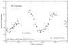 |
Fig. A.1 Composite lightcurve of 281 Lucretia from its 2003 opposition. |
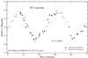 |
Fig. A.2 Composite lightcurve of 281 Lucretia from its 2006 opposition. |
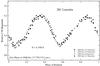 |
Fig. A.3 Composite lightcurve of 281 Lucretia from its 2008/2009 opposition. |
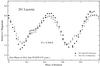 |
Fig. A.4 Composite lightcurve of 281 Lucretia from its 2011 opposition. |
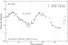 |
Fig. A.5 Composite lightcurve of 291 Alice from its 1999 opposition. |
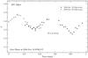 |
Fig. A.6 Composite lightcurve of 291 Alice from its 2004 opposition. |
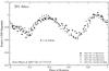 |
Fig. A.7 Composite lightcurve of 291 Alice from its 2007 opposition. |
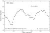 |
Fig. A.8 Composite lightcurve of 291 Alice from its 2009 opposition. |
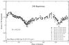 |
Fig. A.9 Composite lightcurve of 298 Baptistina from its 2008 opposition. |
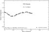 |
Fig. A.10 Composite lightcurve of 352 Gisela from its 2004 opposition. |
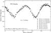 |
Fig. A.11 Composite lightcurve of 352 Gisela from its 2005 opposition. |
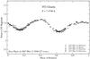 |
Fig. A.12 Composite lightcurve of 352 Gisela from its 2007 opposition. |
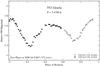 |
Fig. A.13 Composite lightcurve of 352 Gisela from its 2008 opposition. |
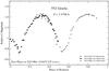 |
Fig. A.14 Composite lightcurve of 352 Gisela from its 2010 opposition. |
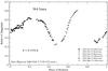 |
Fig. A.15 Composite lightcurve of 364 Isara from its 2005 opposition. |
 |
Fig. A.16 Composite lightcurve of 364 Isara from its 2006 opposition. |
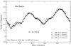 |
Fig. A.17 Composite lightcurve of 364 Isara from its 2009 opposition. ‘ |
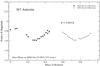 |
Fig. A.18 Composite lightcurve of 367 Amicitia from its 2000 opposition. |
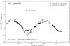 |
Fig. A.19 Composite lightcurve of 367 Amicitia from its 2003 opposition. |
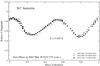 |
Fig. A.20 Composite lightcurve of 367 Amicitia from its 2005 opposition. |
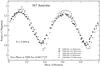 |
Fig. A.21 Composite lightcurve of 367 Amicitia from its 2008 opposition. |
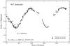 |
Fig. A.22 Composite lightcurve of 367 Amicitia from its 2009 opposition. |
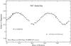 |
Fig. A.23 Composite lightcurve of 367 Amicitia from its 2010 opposition. |
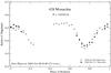 |
Fig. A.24 Composite lightcurve of 428 Monachia from its 2009 opposition. |
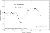 |
Fig. A.25 Composite lightcurve of 428 Monachia from its 2011 opposition. |
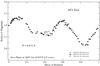 |
Fig. A.26 Composite lightcurve of 453 Tea from its 2005 opposition. |
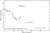 |
Fig. A.27 Composite lightcurve of 453 Tea from its 2006 opposition. |
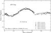 |
Fig. A.28 Composite lightcurve of 453 Tea from its 2008 opposition. |
 |
Fig. A.29 Composite lightcurve of 453 Tea from its 2010 opposition. |
 |
Fig. A.30 Composite lightcurve of 453 Tea from its 2011 opposition. |
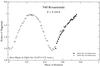 |
Fig. A.31 Composite lightcurve of 540 Rosamunde from its 2004 opposition. |
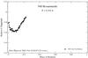 |
Fig. A.32 Composite lightcurve of 540 Rosamunde from its 2007 opposition. |
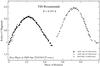 |
Fig. A.33 Composite lightcurve of 540 Rosamunde from its 2009 opposition. |
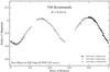 |
Fig. A.34 Composite lightcurve of 540 Rosamunde from its 2010 opposition. |
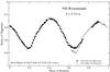 |
Fig. A.35 Composite lightcurve of 540 Rosamunde from its 2012 opposition. |
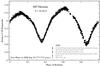 |
Fig. A.36 Composite lightcurve of 685 Hermia from its 2006 opposition. |
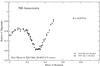 |
Fig. A.37 Composite lightcurve of 700 Auravictrix from its 2003 opposition. |
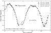 |
Fig. A.38 Composite lightcurve of 700 Auravictrix from its 2004 opposition. |
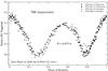 |
Fig. A.39 Composite lightcurve of 700 Auravictrix from its 2006 opposition. |
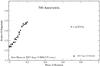 |
Fig. A.40 Composite lightcurve of 700 Auravictrix from its 2007 opposition. |
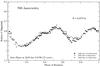 |
Fig. A.41 Composite lightcurve of 700 Auravictrix from its 2008/2009 opposition. |
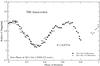 |
Fig. A.42 Composite lightcurve of 700 Auravictrix from its 2011 opposition. |
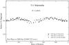 |
Fig. A.43 Composite lightcurve of 711 Marmulla from its 2009 opposition. |
 |
Fig. A.44 Composite lightcurve of 770 Bali from its 2004 opposition. |
 |
Fig. A.45 Composite lightcurve of 770 Bali from its 2007 opposition. |
 |
Fig. A.46 Composite lightcurve of 770 Bali from its 2008 opposition. |
 |
Fig. A.47 Composite lightcurve of 770 Bali from its 2009/2010 opposition. |
 |
Fig. A.48 Composite lightcurve of 770 Bali from its 2011 opposition. |
 |
Fig. A.49 Composite lightcurve of 800 Kressmannia from its 2004 opposition. |
 |
Fig. A.50 Composite lightcurve of 800 Kressmannia from its 2006 opposition. |
 |
Fig. A.51 Composite lightcurve of 800 Kressmannia from its 2007 opposition. |
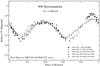 |
Fig. A.52 Composite lightcurve of 800 Kressmannia from its 2009 opposition. |
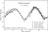 |
Fig. A.53 Composite lightcurve of 800 Kressmannia from its 2010 opposition. |
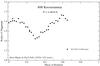 |
Fig. A.54 Composite lightcurve of 800 Kressmannia from its 2012 opposition. |
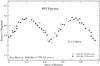 |
Fig. A.55 Composite lightcurve of 802 Epyaxa from its 2006 opposition. |
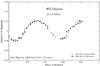 |
Fig. A.56 Composite lightcurve of 802 Epyaxa from its 2009 opposition. |
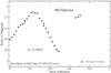 |
Fig. A.57 Composite lightcurve of 802 Epyaxa from its 2010 opposition. |
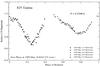 |
Fig. A.58 Composite lightcurve of 825 Tanina from its 1999 opposition. |
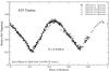 |
Fig. A.59 Composite lightcurve of 825 Tanina from its 2002 opposition. |
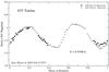 |
Fig. A.60 Composite lightcurve of 825 Tanina from its 2004/2005 opposition. |
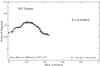 |
Fig. A.61 Composite lightcurve of 825 Tanina from its 2006 opposition. |
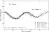 |
Fig. A.62 Composite lightcurve of 825 Tanina from its 2007 opposition. |
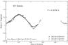 |
Fig. A.63 Composite lightcurve of 825 Tanina from its 2009 opposition. |
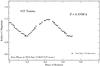 |
Fig. A.64 Composite lightcurve of 825 Tanina from its 2010 opposition. |
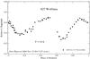 |
Fig. A.65 Composite lightcurve of 827 Wolfiana from its 2009 opposition. |
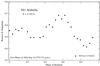 |
Fig. A.66 Composite lightcurve of 841 Arabella from its 2004 opposition. |
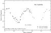 |
Fig. A.67 Composite lightcurve of 841 Arabella from its 2007 opposition. |
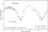 |
Fig. A.68 Composite lightcurve of 864 Aase from its 2007 opposition. |
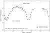 |
Fig. A.69 Composite lightcurve of 864 Aase from its 2009 opposition. |
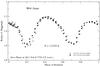 |
Fig. A.70 Composite lightcurve of 864 Aase from its 2010/2011 opposition. |
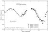 |
Fig. A.71 Composite lightcurve of 905 Universitas from 2004 opposition. |
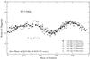 |
Fig. A.72 Composite lightcurve of 913 Otila from its 2010 opposition. |
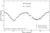 |
Fig. A.73 Composite lightcurve of 915 Cosette from its 2004 opposition. |
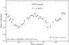 |
Fig. A.74 Composite lightcurve of 915 Cosette from its 2006 opposition. |
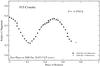 |
Fig. A.75 Composite lightcurve of 915 Cosette from its 2008 opposition. |
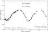 |
Fig. A.76 Composite lightcurve of 915 Cosette from its 2010 opposition. |
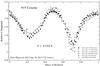 |
Fig. A.77 Composite lightcurve of 915 Cosette from its 2011/2012 opposition. |
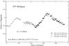 |
Fig. A.78 Composite lightcurve of 937 Bethgea from its 2000 opposition. |
 |
Fig. A.79 Composite lightcurve of 937 Bethgea from its 2004 opposition. |
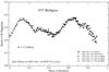 |
Fig. A.80 Composite lightcurve of 937 Bethgea from its 2007 opposition. |
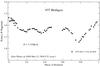 |
Fig. A.81 Composite lightcurve of 937 Bethgea from its 2009 opposition. |
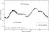 |
Fig. A.82 Composite lightcurve of 937 Bethgea from its 2010 opposition. |
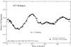 |
Fig. A.83 Composite lightcurve of 937 Bethgea from its 2012 opposition. |
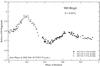 |
Fig. A.84 Composite lightcurve of 960 Birgit from its 2007 opposition. |
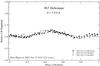 |
Fig. A.85 Composite lightcurve of 967 Helionape from its 2007 opposition. |
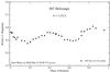 |
Fig. A.86 Composite lightcurve of 967 Helionape from its 2009 opposition. |
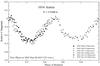 |
Fig. A.87 Composite lightcurve of 1016 Anitra from its 2005 opposition. |
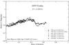 |
Fig. A.88 Composite lightcurve of 1055 Tynka from its 2009 opposition. |
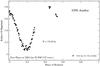 |
Fig. A.89 Composite lightcurve of 1056 Azalea from its 2004 opposition. |
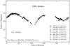 |
Fig. A.90 Composite lightcurve of 1056 Azalea from its 2008 opposition. |
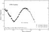 |
Fig. A.91 Composite lightcurve of 1056 Azalea from its 2011 opposition. |
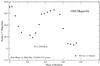 |
Fig. A.92 Composite lightcurve of 1060 Magnolia from its 2002 opposition. |
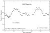 |
Fig. A.93 Composite lightcurve of 1060 Magnolia from its 2005 opposition. |
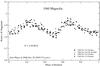 |
Fig. A.94 Composite lightcurve of 1060 Magnolia from its 2006 opposition. |
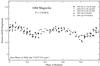 |
Fig. A.95 Composite lightcurve of 1060 Magnolia from its 2008 opposition. |
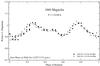 |
Fig. A.96 Composite lightcurve of 1060 Magnolia from its 2009 opposition. |
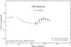 |
Fig. A.97 Composite lightcurve of 1060 Magnolia from its 2011 opposition. |
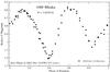 |
Fig. A.98 Composite lightcurve of 1088 Mitaka from its 2002 opposition. |
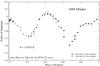 |
Fig. A.99 Composite lightcurve of 1088 Mitaka from its 2004 opposition. |
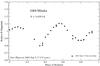 |
Fig. A.100 Composite lightcurve of 1088 Mitaka from its 2005 opposition. |
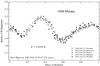 |
Fig. A.101 Composite lightcurve of 1088 Mitaka from its 2006/2007 opposition. |
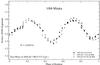 |
Fig. A.102 Composite lightcurve of 1088 Mitaka from its 2008 opposition. |
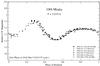 |
Fig. A.103 Composite lightcurve of 1088 Mitaka from its 2009/2010 opposition. |
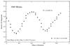 |
Fig. A.104 Composite lightcurve of 1088 Mitaka from its 2011 opposition. |
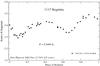 |
Fig. A.105 Composite lightcurve of 1117 Reginita from its 2002 opposition. |
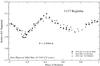 |
Fig. A.106 Composite lightcurve of 1117 Reginita from its 2004 opposition. |
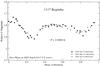 |
Fig. A.107 Composite lightcurve of 1117 Reginita from its 2005 opposition. |
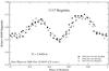 |
Fig. A.108 Composite lightcurve of 1117 Reginita from its 2006/2007 opposition. |
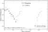 |
Fig. A.109 Composite lightcurve of 1117 Reginita from its 2008 opposition. |
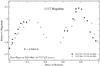 |
Fig. A.110 Composite lightcurve of 1117 Reginita from its 2009/2010 opposition. |
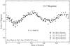 |
Fig. A.111 Composite lightcurve of 1117 Reginita from its 2011 opposition. |
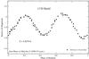 |
Fig. A.112 Composite lightcurve of 1130 Skuld from its 2004 opposition. |
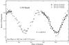 |
Fig. A.113 Composite lightcurve of 1130 Skuld from its 2006/2007 opposition. |
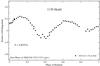 |
Fig. A.114 Composite lightcurve of 1130 Skuld from its 2008 opposition. |
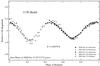 |
Fig. A.115 Composite lightcurve of 1130 Skuld from its 2009 opposition. |
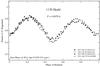 |
Fig. A.116 Composite lightcurve of 1130 Skuld from its 2011 opposition. |
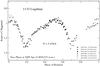 |
Fig. A.117 Composite lightcurve of 1133 Lugduna from its 2009 opposition. |
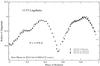 |
Fig. A.118 Composite lightcurve of 1133 Lugduna from its 2010 opposition. |
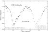 |
Fig. A.119 Composite lightcurve of 1188 Gothlandia from its 2006 opposition. |
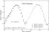 |
Fig. A.120 Composite lightcurve of 1188 Gothlandia from its 2008/2009 opposition. |
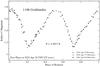 |
Fig. A.121 Composite lightcurve of 1188 Gothlandia from its 2010 opposition. |
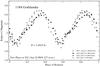 |
Fig. A.122 Composite lightcurve of 1188 Gothlandia from its 2011/2012 opposition. |
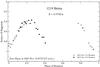 |
Fig. A.123 Composite lightcurve of 1219 Britta from its 2003 opposition. |
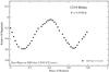 |
Fig. A.124 Composite lightcurve of 1219 Britta from its 2005 opposition. |
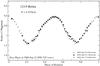 |
Fig. A.125 Composite lightcurve of 1219 Britta from its 2006 opposition. |
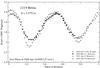 |
Fig. A.126 Composite lightcurve of 1219 Britta from its 2008 opposition. |
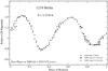 |
Fig. A.127 Composite lightcurve of 1219 Britta from its 2009 opposition. |
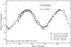 |
Fig. A.128 Composite lightcurve of 1219 Britta from its 2010/2011 opposition. |
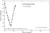 |
Fig. A.129 Composite lightcurve of 1249 Rutherfordia from its 2005 opposition. |
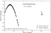 |
Fig. A.130 Composite lightcurve of 1249 Rutherfordia from its 2008 opposition. |
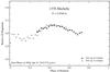 |
Fig. A.131 Composite lightcurve of 1376 Michelle from its 2004 opposition. |
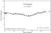 |
Fig. A.132 Composite lightcurve of 1376 Michelle from its 2005 opposition. |
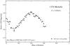 |
Fig. A.133 Composite lightcurve of 1376 Michelle from its 2007 opposition. |
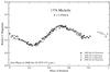 |
Fig. A.134 Composite lightcurve of 1376 Michelle from its 2008 opposition. |
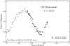 |
Fig. A.135 Composite lightcurve of 1523 Pieksamaki from its 2004 opposition. |
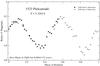 |
Fig. A.136 Composite lightcurve of 1523 Pieksamaki from its 2006 opposition. |
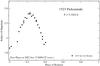 |
Fig. A.137 Composite lightcurve of 1523 Pieksamaki from its 2007 opposition. |
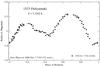 |
Fig. A.138 Composite lightcurve of 1523 Pieksamaki from its 2008 opposition. |
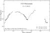 |
Fig. A.139 Composite lightcurve of 1523 Pieksamaki from its 2010 opposition. |
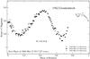 |
Fig. A.140 Composite lightcurve of 1562 Gondolatsch from its 2006 opposition. |
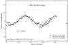 |
Fig. A.141 Composite lightcurve of 1590 Tsiolkovskaja from its 2007/2008 opposition. |
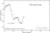 |
Fig. A.142 Composite lightcurve of 1590 Tsiolkovskaja from its 2010 opposition. |
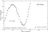 |
Fig. A.143 Composite lightcurve of 1601 Patry from its 2009 opposition. |
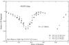 |
Fig. A.144 Composite lightcurve of 1619 from its 2009 opposition. |
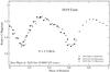 |
Fig. A.145 Composite lightcurve of 1619 from its 2010 opposition. |
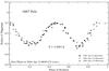 |
Fig. A.146 Composite lightcurve of 1667 Pels from its 2004 opposition. |
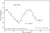 |
Fig. A.147 Composite lightcurve of 1667 Pels from its 2005 opposition. |
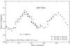 |
Fig. A.148 Composite lightcurve of 1667 Pels from its 2007 opposition. |
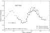 |
Fig. A.149 Composite lightcurve of 1667 Pels from its 2008/2009 opposition. |
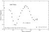 |
Fig. A.150 Composite lightcurve of 1667 Pels from its 2010 opposition. |
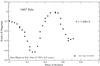 |
Fig. A.151 Composite lightcurve of 1667 Pels from its 2011 opposition. |
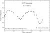 |
Fig. A.152 Composite lightcurve of 1675 Simonida from its 2004 opposition. |
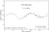 |
Fig. A.153 Composite lightcurve of 1675 Simonida from its 2005 opposition. |
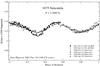 |
Fig. A.154 Composite lightcurve of 1675 Simonida from its 2007/2008 opposition. |
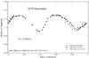 |
Fig. A.155 Composite lightcurve of 1675 Simonida from its 2009 opposition. |
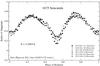 |
Fig. A.156 Composite lightcurve of 1675 Simonida from its 2010/2011 opposition. |
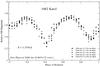 |
Fig. A.157 Composite lightcurve of 1682 Karel from its 2008 opposition. |
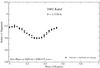 |
Fig. A.158 Composite lightcurve of 1682 Karel from its 2009 opposition. |
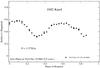 |
Fig. A.159 Composite lightcurve of 1682 Karel from its 2010 opposition. |
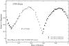 |
Fig. A.160 Composite lightcurve of 1793 Zoya from its 2011 opposition. |
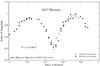 |
Fig. A.161 Composite lightcurve of 2017 Wesson from its 2004 opposition. |
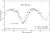 |
Fig. A.162 Composite lightcurve of 2017 Wesson from its 2005/2006 opposition. |
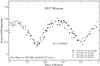 |
Fig. A.163 Composite lightcurve of 2017 Wesson from its 2007 opposition. |
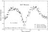 |
Fig. A.164 Composite lightcurve of 2017 Wesson from its 2008/2009 opposition. |
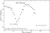 |
Fig. A.165 Composite lightcurve of 2017 Wesson from its 2010 opposition. |
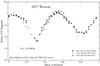 |
Fig. A.166 Composite lightcurve of 2017 Wesson from its 2011 opposition. |
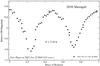 |
Fig. A.167 Composite lightcurve of 2036 Sheragul from its 2007 opposition. |
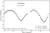 |
Fig. A.168 Composite lightcurve of 2156 Kate from its 2001 opposition. |
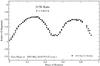 |
Fig. A.169 Composite lightcurve of 2156 Kate from its 2003 opposition. |
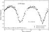 |
Fig. A.170 Composite lightcurve of 2156 Kate from its 2006 opposition. |
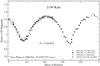 |
Fig. A.171 Composite lightcurve of 2156 Kate from its 2008/2009 opposition. |
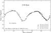 |
Fig. A.172 Composite lightcurve of 2156 Kate from its 2010 opposition. |
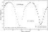 |
Fig. A.173 Composite lightcurve of 2156 Kate from its 2011 opposition. |
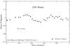 |
Fig. A.174 Composite lightcurve of 2283 Bunke from its 2004 opposition. |
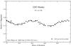 |
Fig. A.175 Composite lightcurve of 2283 Bunke from its 2009 opposition. |
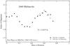 |
Fig. A.176 Composite lightcurve of 2460 Mitlincoln its from 2004 opposition. |
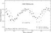 |
Fig. A.177 Composite lightcurve of 2460 Mitlincoln from its 2007 opposition. |
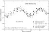 |
Fig. A.178 Composite lightcurve of 2460 Mitlincoln from its 2009 opposition. |
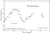 |
Fig. A.179 Composite lightcurve of 2961 Katsurahama from its 2006 opposition. |
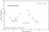 |
Fig. A.180 Composite lightcurve of 2961 Katsurahama from its 2008 opposition. |
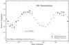 |
Fig. A.181 Composite lightcurve of 2961 Katsurahama from its 2009 opposition. |
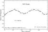 |
Fig. A.182 Composite lightcurve of 3953 Perth from its 2008 opposition. |
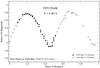 |
Fig. A.183 Composite lightcurve of 3953 Perth from its 2009 opposition. |
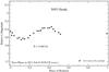 |
Fig. A.184 Composite lightcurve of 3953 Perth from its 2011 opposition. |
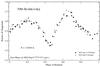 |
Fig. A.185 Composite lightcurve of 3986 Rozhkovskij from its 2005 opposition. |
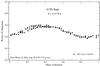 |
Fig. A.186 Composite lightcurve of 4150 Starr from its 2004 opposition. |
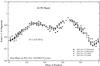 |
Fig. A.187 Composite lightcurve of 4150 Starr from its 2011 opposition. |
Aspect data.
continued.
All Tables
All Figures
|
Fig. 1 Absolute magnitude H (mag) as a function of semimajor axis a (AU) for 146. Flora family asteroids. |
| In the text | |
|
Fig. 2 Histogram of the diameters of the Flora family objects from our sample, the largest objects 8 Flora (138 km), 9 Metis (166 km), 43 Ariadne (59 km), and 113 Amalthea (46 km) are excluded. |
| In the text | |
|
Fig. 3 Solid line – observed rotation-rate distribution for 142 objects of the Flora family. Asteroids observed within this campain are marked in grey. The dashed curve represents the Maxwellian distribution, for a mean squared frequency of 5.47 1/d, which is inconsistent with the sample at the 94% confidence level. The asteroids 8 Flora, 9 Metis, 43 Ariadne and 113 Amalthea are excluded. |
| In the text | |
|
Fig. 4 Observed rotation-rate distribution for objects of the Flora family classified by different methods. 8 Flora, 9 Metis, 43 Ariadne, and 113 Amalthea are excluded. |
| In the text | |
|
Fig. 5 Relation between frequency of rotation and diameter for 146 Flora family objects. All objects larger than 16 km rotate slower than 5 cycles per day. Smaller objects present all possible variety of frequencies. |
| In the text | |
|
Fig. A.1 Composite lightcurve of 281 Lucretia from its 2003 opposition. |
| In the text | |
|
Fig. A.2 Composite lightcurve of 281 Lucretia from its 2006 opposition. |
| In the text | |
|
Fig. A.3 Composite lightcurve of 281 Lucretia from its 2008/2009 opposition. |
| In the text | |
|
Fig. A.4 Composite lightcurve of 281 Lucretia from its 2011 opposition. |
| In the text | |
|
Fig. A.5 Composite lightcurve of 291 Alice from its 1999 opposition. |
| In the text | |
|
Fig. A.6 Composite lightcurve of 291 Alice from its 2004 opposition. |
| In the text | |
|
Fig. A.7 Composite lightcurve of 291 Alice from its 2007 opposition. |
| In the text | |
|
Fig. A.8 Composite lightcurve of 291 Alice from its 2009 opposition. |
| In the text | |
|
Fig. A.9 Composite lightcurve of 298 Baptistina from its 2008 opposition. |
| In the text | |
|
Fig. A.10 Composite lightcurve of 352 Gisela from its 2004 opposition. |
| In the text | |
|
Fig. A.11 Composite lightcurve of 352 Gisela from its 2005 opposition. |
| In the text | |
|
Fig. A.12 Composite lightcurve of 352 Gisela from its 2007 opposition. |
| In the text | |
|
Fig. A.13 Composite lightcurve of 352 Gisela from its 2008 opposition. |
| In the text | |
|
Fig. A.14 Composite lightcurve of 352 Gisela from its 2010 opposition. |
| In the text | |
|
Fig. A.15 Composite lightcurve of 364 Isara from its 2005 opposition. |
| In the text | |
|
Fig. A.16 Composite lightcurve of 364 Isara from its 2006 opposition. |
| In the text | |
|
Fig. A.17 Composite lightcurve of 364 Isara from its 2009 opposition. ‘ |
| In the text | |
|
Fig. A.18 Composite lightcurve of 367 Amicitia from its 2000 opposition. |
| In the text | |
|
Fig. A.19 Composite lightcurve of 367 Amicitia from its 2003 opposition. |
| In the text | |
|
Fig. A.20 Composite lightcurve of 367 Amicitia from its 2005 opposition. |
| In the text | |
|
Fig. A.21 Composite lightcurve of 367 Amicitia from its 2008 opposition. |
| In the text | |
|
Fig. A.22 Composite lightcurve of 367 Amicitia from its 2009 opposition. |
| In the text | |
|
Fig. A.23 Composite lightcurve of 367 Amicitia from its 2010 opposition. |
| In the text | |
|
Fig. A.24 Composite lightcurve of 428 Monachia from its 2009 opposition. |
| In the text | |
|
Fig. A.25 Composite lightcurve of 428 Monachia from its 2011 opposition. |
| In the text | |
|
Fig. A.26 Composite lightcurve of 453 Tea from its 2005 opposition. |
| In the text | |
|
Fig. A.27 Composite lightcurve of 453 Tea from its 2006 opposition. |
| In the text | |
|
Fig. A.28 Composite lightcurve of 453 Tea from its 2008 opposition. |
| In the text | |
|
Fig. A.29 Composite lightcurve of 453 Tea from its 2010 opposition. |
| In the text | |
|
Fig. A.30 Composite lightcurve of 453 Tea from its 2011 opposition. |
| In the text | |
|
Fig. A.31 Composite lightcurve of 540 Rosamunde from its 2004 opposition. |
| In the text | |
|
Fig. A.32 Composite lightcurve of 540 Rosamunde from its 2007 opposition. |
| In the text | |
|
Fig. A.33 Composite lightcurve of 540 Rosamunde from its 2009 opposition. |
| In the text | |
|
Fig. A.34 Composite lightcurve of 540 Rosamunde from its 2010 opposition. |
| In the text | |
|
Fig. A.35 Composite lightcurve of 540 Rosamunde from its 2012 opposition. |
| In the text | |
|
Fig. A.36 Composite lightcurve of 685 Hermia from its 2006 opposition. |
| In the text | |
|
Fig. A.37 Composite lightcurve of 700 Auravictrix from its 2003 opposition. |
| In the text | |
|
Fig. A.38 Composite lightcurve of 700 Auravictrix from its 2004 opposition. |
| In the text | |
|
Fig. A.39 Composite lightcurve of 700 Auravictrix from its 2006 opposition. |
| In the text | |
|
Fig. A.40 Composite lightcurve of 700 Auravictrix from its 2007 opposition. |
| In the text | |
|
Fig. A.41 Composite lightcurve of 700 Auravictrix from its 2008/2009 opposition. |
| In the text | |
|
Fig. A.42 Composite lightcurve of 700 Auravictrix from its 2011 opposition. |
| In the text | |
|
Fig. A.43 Composite lightcurve of 711 Marmulla from its 2009 opposition. |
| In the text | |
|
Fig. A.44 Composite lightcurve of 770 Bali from its 2004 opposition. |
| In the text | |
|
Fig. A.45 Composite lightcurve of 770 Bali from its 2007 opposition. |
| In the text | |
|
Fig. A.46 Composite lightcurve of 770 Bali from its 2008 opposition. |
| In the text | |
|
Fig. A.47 Composite lightcurve of 770 Bali from its 2009/2010 opposition. |
| In the text | |
|
Fig. A.48 Composite lightcurve of 770 Bali from its 2011 opposition. |
| In the text | |
|
Fig. A.49 Composite lightcurve of 800 Kressmannia from its 2004 opposition. |
| In the text | |
|
Fig. A.50 Composite lightcurve of 800 Kressmannia from its 2006 opposition. |
| In the text | |
|
Fig. A.51 Composite lightcurve of 800 Kressmannia from its 2007 opposition. |
| In the text | |
|
Fig. A.52 Composite lightcurve of 800 Kressmannia from its 2009 opposition. |
| In the text | |
|
Fig. A.53 Composite lightcurve of 800 Kressmannia from its 2010 opposition. |
| In the text | |
|
Fig. A.54 Composite lightcurve of 800 Kressmannia from its 2012 opposition. |
| In the text | |
|
Fig. A.55 Composite lightcurve of 802 Epyaxa from its 2006 opposition. |
| In the text | |
|
Fig. A.56 Composite lightcurve of 802 Epyaxa from its 2009 opposition. |
| In the text | |
|
Fig. A.57 Composite lightcurve of 802 Epyaxa from its 2010 opposition. |
| In the text | |
|
Fig. A.58 Composite lightcurve of 825 Tanina from its 1999 opposition. |
| In the text | |
|
Fig. A.59 Composite lightcurve of 825 Tanina from its 2002 opposition. |
| In the text | |
|
Fig. A.60 Composite lightcurve of 825 Tanina from its 2004/2005 opposition. |
| In the text | |
|
Fig. A.61 Composite lightcurve of 825 Tanina from its 2006 opposition. |
| In the text | |
|
Fig. A.62 Composite lightcurve of 825 Tanina from its 2007 opposition. |
| In the text | |
|
Fig. A.63 Composite lightcurve of 825 Tanina from its 2009 opposition. |
| In the text | |
|
Fig. A.64 Composite lightcurve of 825 Tanina from its 2010 opposition. |
| In the text | |
|
Fig. A.65 Composite lightcurve of 827 Wolfiana from its 2009 opposition. |
| In the text | |
|
Fig. A.66 Composite lightcurve of 841 Arabella from its 2004 opposition. |
| In the text | |
|
Fig. A.67 Composite lightcurve of 841 Arabella from its 2007 opposition. |
| In the text | |
|
Fig. A.68 Composite lightcurve of 864 Aase from its 2007 opposition. |
| In the text | |
|
Fig. A.69 Composite lightcurve of 864 Aase from its 2009 opposition. |
| In the text | |
|
Fig. A.70 Composite lightcurve of 864 Aase from its 2010/2011 opposition. |
| In the text | |
|
Fig. A.71 Composite lightcurve of 905 Universitas from 2004 opposition. |
| In the text | |
|
Fig. A.72 Composite lightcurve of 913 Otila from its 2010 opposition. |
| In the text | |
|
Fig. A.73 Composite lightcurve of 915 Cosette from its 2004 opposition. |
| In the text | |
|
Fig. A.74 Composite lightcurve of 915 Cosette from its 2006 opposition. |
| In the text | |
|
Fig. A.75 Composite lightcurve of 915 Cosette from its 2008 opposition. |
| In the text | |
|
Fig. A.76 Composite lightcurve of 915 Cosette from its 2010 opposition. |
| In the text | |
|
Fig. A.77 Composite lightcurve of 915 Cosette from its 2011/2012 opposition. |
| In the text | |
|
Fig. A.78 Composite lightcurve of 937 Bethgea from its 2000 opposition. |
| In the text | |
|
Fig. A.79 Composite lightcurve of 937 Bethgea from its 2004 opposition. |
| In the text | |
|
Fig. A.80 Composite lightcurve of 937 Bethgea from its 2007 opposition. |
| In the text | |
|
Fig. A.81 Composite lightcurve of 937 Bethgea from its 2009 opposition. |
| In the text | |
|
Fig. A.82 Composite lightcurve of 937 Bethgea from its 2010 opposition. |
| In the text | |
|
Fig. A.83 Composite lightcurve of 937 Bethgea from its 2012 opposition. |
| In the text | |
|
Fig. A.84 Composite lightcurve of 960 Birgit from its 2007 opposition. |
| In the text | |
|
Fig. A.85 Composite lightcurve of 967 Helionape from its 2007 opposition. |
| In the text | |
|
Fig. A.86 Composite lightcurve of 967 Helionape from its 2009 opposition. |
| In the text | |
|
Fig. A.87 Composite lightcurve of 1016 Anitra from its 2005 opposition. |
| In the text | |
|
Fig. A.88 Composite lightcurve of 1055 Tynka from its 2009 opposition. |
| In the text | |
|
Fig. A.89 Composite lightcurve of 1056 Azalea from its 2004 opposition. |
| In the text | |
|
Fig. A.90 Composite lightcurve of 1056 Azalea from its 2008 opposition. |
| In the text | |
|
Fig. A.91 Composite lightcurve of 1056 Azalea from its 2011 opposition. |
| In the text | |
|
Fig. A.92 Composite lightcurve of 1060 Magnolia from its 2002 opposition. |
| In the text | |
|
Fig. A.93 Composite lightcurve of 1060 Magnolia from its 2005 opposition. |
| In the text | |
|
Fig. A.94 Composite lightcurve of 1060 Magnolia from its 2006 opposition. |
| In the text | |
|
Fig. A.95 Composite lightcurve of 1060 Magnolia from its 2008 opposition. |
| In the text | |
|
Fig. A.96 Composite lightcurve of 1060 Magnolia from its 2009 opposition. |
| In the text | |
|
Fig. A.97 Composite lightcurve of 1060 Magnolia from its 2011 opposition. |
| In the text | |
|
Fig. A.98 Composite lightcurve of 1088 Mitaka from its 2002 opposition. |
| In the text | |
|
Fig. A.99 Composite lightcurve of 1088 Mitaka from its 2004 opposition. |
| In the text | |
|
Fig. A.100 Composite lightcurve of 1088 Mitaka from its 2005 opposition. |
| In the text | |
|
Fig. A.101 Composite lightcurve of 1088 Mitaka from its 2006/2007 opposition. |
| In the text | |
|
Fig. A.102 Composite lightcurve of 1088 Mitaka from its 2008 opposition. |
| In the text | |
|
Fig. A.103 Composite lightcurve of 1088 Mitaka from its 2009/2010 opposition. |
| In the text | |
|
Fig. A.104 Composite lightcurve of 1088 Mitaka from its 2011 opposition. |
| In the text | |
|
Fig. A.105 Composite lightcurve of 1117 Reginita from its 2002 opposition. |
| In the text | |
|
Fig. A.106 Composite lightcurve of 1117 Reginita from its 2004 opposition. |
| In the text | |
|
Fig. A.107 Composite lightcurve of 1117 Reginita from its 2005 opposition. |
| In the text | |
|
Fig. A.108 Composite lightcurve of 1117 Reginita from its 2006/2007 opposition. |
| In the text | |
|
Fig. A.109 Composite lightcurve of 1117 Reginita from its 2008 opposition. |
| In the text | |
|
Fig. A.110 Composite lightcurve of 1117 Reginita from its 2009/2010 opposition. |
| In the text | |
|
Fig. A.111 Composite lightcurve of 1117 Reginita from its 2011 opposition. |
| In the text | |
|
Fig. A.112 Composite lightcurve of 1130 Skuld from its 2004 opposition. |
| In the text | |
|
Fig. A.113 Composite lightcurve of 1130 Skuld from its 2006/2007 opposition. |
| In the text | |
|
Fig. A.114 Composite lightcurve of 1130 Skuld from its 2008 opposition. |
| In the text | |
|
Fig. A.115 Composite lightcurve of 1130 Skuld from its 2009 opposition. |
| In the text | |
|
Fig. A.116 Composite lightcurve of 1130 Skuld from its 2011 opposition. |
| In the text | |
|
Fig. A.117 Composite lightcurve of 1133 Lugduna from its 2009 opposition. |
| In the text | |
|
Fig. A.118 Composite lightcurve of 1133 Lugduna from its 2010 opposition. |
| In the text | |
|
Fig. A.119 Composite lightcurve of 1188 Gothlandia from its 2006 opposition. |
| In the text | |
|
Fig. A.120 Composite lightcurve of 1188 Gothlandia from its 2008/2009 opposition. |
| In the text | |
|
Fig. A.121 Composite lightcurve of 1188 Gothlandia from its 2010 opposition. |
| In the text | |
|
Fig. A.122 Composite lightcurve of 1188 Gothlandia from its 2011/2012 opposition. |
| In the text | |
|
Fig. A.123 Composite lightcurve of 1219 Britta from its 2003 opposition. |
| In the text | |
|
Fig. A.124 Composite lightcurve of 1219 Britta from its 2005 opposition. |
| In the text | |
|
Fig. A.125 Composite lightcurve of 1219 Britta from its 2006 opposition. |
| In the text | |
|
Fig. A.126 Composite lightcurve of 1219 Britta from its 2008 opposition. |
| In the text | |
|
Fig. A.127 Composite lightcurve of 1219 Britta from its 2009 opposition. |
| In the text | |
|
Fig. A.128 Composite lightcurve of 1219 Britta from its 2010/2011 opposition. |
| In the text | |
|
Fig. A.129 Composite lightcurve of 1249 Rutherfordia from its 2005 opposition. |
| In the text | |
|
Fig. A.130 Composite lightcurve of 1249 Rutherfordia from its 2008 opposition. |
| In the text | |
|
Fig. A.131 Composite lightcurve of 1376 Michelle from its 2004 opposition. |
| In the text | |
|
Fig. A.132 Composite lightcurve of 1376 Michelle from its 2005 opposition. |
| In the text | |
|
Fig. A.133 Composite lightcurve of 1376 Michelle from its 2007 opposition. |
| In the text | |
|
Fig. A.134 Composite lightcurve of 1376 Michelle from its 2008 opposition. |
| In the text | |
|
Fig. A.135 Composite lightcurve of 1523 Pieksamaki from its 2004 opposition. |
| In the text | |
|
Fig. A.136 Composite lightcurve of 1523 Pieksamaki from its 2006 opposition. |
| In the text | |
|
Fig. A.137 Composite lightcurve of 1523 Pieksamaki from its 2007 opposition. |
| In the text | |
|
Fig. A.138 Composite lightcurve of 1523 Pieksamaki from its 2008 opposition. |
| In the text | |
|
Fig. A.139 Composite lightcurve of 1523 Pieksamaki from its 2010 opposition. |
| In the text | |
|
Fig. A.140 Composite lightcurve of 1562 Gondolatsch from its 2006 opposition. |
| In the text | |
|
Fig. A.141 Composite lightcurve of 1590 Tsiolkovskaja from its 2007/2008 opposition. |
| In the text | |
|
Fig. A.142 Composite lightcurve of 1590 Tsiolkovskaja from its 2010 opposition. |
| In the text | |
|
Fig. A.143 Composite lightcurve of 1601 Patry from its 2009 opposition. |
| In the text | |
|
Fig. A.144 Composite lightcurve of 1619 from its 2009 opposition. |
| In the text | |
|
Fig. A.145 Composite lightcurve of 1619 from its 2010 opposition. |
| In the text | |
|
Fig. A.146 Composite lightcurve of 1667 Pels from its 2004 opposition. |
| In the text | |
|
Fig. A.147 Composite lightcurve of 1667 Pels from its 2005 opposition. |
| In the text | |
|
Fig. A.148 Composite lightcurve of 1667 Pels from its 2007 opposition. |
| In the text | |
|
Fig. A.149 Composite lightcurve of 1667 Pels from its 2008/2009 opposition. |
| In the text | |
|
Fig. A.150 Composite lightcurve of 1667 Pels from its 2010 opposition. |
| In the text | |
|
Fig. A.151 Composite lightcurve of 1667 Pels from its 2011 opposition. |
| In the text | |
|
Fig. A.152 Composite lightcurve of 1675 Simonida from its 2004 opposition. |
| In the text | |
|
Fig. A.153 Composite lightcurve of 1675 Simonida from its 2005 opposition. |
| In the text | |
|
Fig. A.154 Composite lightcurve of 1675 Simonida from its 2007/2008 opposition. |
| In the text | |
|
Fig. A.155 Composite lightcurve of 1675 Simonida from its 2009 opposition. |
| In the text | |
|
Fig. A.156 Composite lightcurve of 1675 Simonida from its 2010/2011 opposition. |
| In the text | |
|
Fig. A.157 Composite lightcurve of 1682 Karel from its 2008 opposition. |
| In the text | |
|
Fig. A.158 Composite lightcurve of 1682 Karel from its 2009 opposition. |
| In the text | |
|
Fig. A.159 Composite lightcurve of 1682 Karel from its 2010 opposition. |
| In the text | |
|
Fig. A.160 Composite lightcurve of 1793 Zoya from its 2011 opposition. |
| In the text | |
|
Fig. A.161 Composite lightcurve of 2017 Wesson from its 2004 opposition. |
| In the text | |
|
Fig. A.162 Composite lightcurve of 2017 Wesson from its 2005/2006 opposition. |
| In the text | |
|
Fig. A.163 Composite lightcurve of 2017 Wesson from its 2007 opposition. |
| In the text | |
|
Fig. A.164 Composite lightcurve of 2017 Wesson from its 2008/2009 opposition. |
| In the text | |
|
Fig. A.165 Composite lightcurve of 2017 Wesson from its 2010 opposition. |
| In the text | |
|
Fig. A.166 Composite lightcurve of 2017 Wesson from its 2011 opposition. |
| In the text | |
|
Fig. A.167 Composite lightcurve of 2036 Sheragul from its 2007 opposition. |
| In the text | |
|
Fig. A.168 Composite lightcurve of 2156 Kate from its 2001 opposition. |
| In the text | |
|
Fig. A.169 Composite lightcurve of 2156 Kate from its 2003 opposition. |
| In the text | |
|
Fig. A.170 Composite lightcurve of 2156 Kate from its 2006 opposition. |
| In the text | |
|
Fig. A.171 Composite lightcurve of 2156 Kate from its 2008/2009 opposition. |
| In the text | |
|
Fig. A.172 Composite lightcurve of 2156 Kate from its 2010 opposition. |
| In the text | |
|
Fig. A.173 Composite lightcurve of 2156 Kate from its 2011 opposition. |
| In the text | |
|
Fig. A.174 Composite lightcurve of 2283 Bunke from its 2004 opposition. |
| In the text | |
|
Fig. A.175 Composite lightcurve of 2283 Bunke from its 2009 opposition. |
| In the text | |
|
Fig. A.176 Composite lightcurve of 2460 Mitlincoln its from 2004 opposition. |
| In the text | |
|
Fig. A.177 Composite lightcurve of 2460 Mitlincoln from its 2007 opposition. |
| In the text | |
|
Fig. A.178 Composite lightcurve of 2460 Mitlincoln from its 2009 opposition. |
| In the text | |
|
Fig. A.179 Composite lightcurve of 2961 Katsurahama from its 2006 opposition. |
| In the text | |
|
Fig. A.180 Composite lightcurve of 2961 Katsurahama from its 2008 opposition. |
| In the text | |
|
Fig. A.181 Composite lightcurve of 2961 Katsurahama from its 2009 opposition. |
| In the text | |
|
Fig. A.182 Composite lightcurve of 3953 Perth from its 2008 opposition. |
| In the text | |
|
Fig. A.183 Composite lightcurve of 3953 Perth from its 2009 opposition. |
| In the text | |
|
Fig. A.184 Composite lightcurve of 3953 Perth from its 2011 opposition. |
| In the text | |
|
Fig. A.185 Composite lightcurve of 3986 Rozhkovskij from its 2005 opposition. |
| In the text | |
|
Fig. A.186 Composite lightcurve of 4150 Starr from its 2004 opposition. |
| In the text | |
|
Fig. A.187 Composite lightcurve of 4150 Starr from its 2011 opposition. |
| In the text | |
Current usage metrics show cumulative count of Article Views (full-text article views including HTML views, PDF and ePub downloads, according to the available data) and Abstracts Views on Vision4Press platform.
Data correspond to usage on the plateform after 2015. The current usage metrics is available 48-96 hours after online publication and is updated daily on week days.
Initial download of the metrics may take a while.