© ESO, 2012

1. Introduction

Solar twins, defined by Cayrel de Strobel et al. (1981), are stars that are practically identical to the Sun. They allow us to carry out a precise differential analysis with regard to the Sun (Ramírez et al. 2009; Meléndez et al. 2009). To perform this analysis, the physical characteristics of the solar twins need to be precisely known. The star 18 Scorpii (HD 146233; HIP 79672; V = 5.5), suggested to be a solar twin by Porto de Mello & Da Silva (1997), has been studied several times. The atmospheric features of 18 Scorpii are similar to those of the Sun (Takeda et al. 2007; Ramírez et al. 2009; Meléndez & Ramírez 2007; Takeda & Tajitsu 2009; Meléndez et al. 2006; Valenti & Fischer 2005). Its rotation rate of 22.7 ± 0.5 d, which was provided by Petit et al. (2008), is also similar to the solar one. Recently, Bazot et al. (2011) found its radius and average large frequency separation, which are 1.010 ± 0.009 R_⊙ and 134.4 ± 0.3 μHz, respectively.

The classical method for obtaining the stellar parameters is to compare theoretical evolutionary models with observed features in the Hertzsprung-Russell (H-R) diagrams. However, this in general makes it difficult to derive self-consistent, complete sets of stellar atmospheric parameters. Stellar structure and evolution models have several free, unconstrained parameters, which added to the uncertainties in the classical observations, lead to insufficient estimates of the masses, ages, and metallicities of stars (Bi et al. 2008).

Currently, asteroseismology has become an ideal tool to test theories of stellar structure and evolution. It is also a powerful technique for constraining stellar parameters. Its observational data, such as the stellar p-mode oscillation spectrum (for solar-like stars), which provides a very good measure of the age and size of the stars, are independent of metallicity in their uncertainty range. Additionally, the surface lithium abundance observed in solar-like stars was considered to be an extraordinarily sensitive diagnostic of stellar structure and evolution, because it is easily burned at the relatively low temperature of  ~2.5 × 10⁶ K in the stellar interior. Accurate lithium abundance measurement and non-standard models are able to provide more precise information about stellar parameters than determined by classical methods alone. do Nascimento et al. (2009) first used the lithium abundance to constrain mass and age of solar twins with rotating models. Subsequently, Castro et al. (2011) and Li et al. (2012) used the same method to study solar analogs and twins in M67 and solar analogs and twins in the field.

In this work, we constructed evolutionary models including microscopic diffusion and rotationally driven mixing. Based on four classical observed constraints (T_eff, L, [Fe/H] and R), two additional observed limits, lithium abundance log N(Li) and an average large frequency ⟨△ν⟩ , were considered for constraining more accurate stellar parameters. Because a rotating model is used in our analysis, the theoretical models should also fit the observed rotational period ${\mathit{P}}_{\mathrm{rot}}^{\mathrm{eq}}$. However, this parameter cannot be used to constrain the mass and age of the star due to the uncertainty of its evolutionary history.

In Sect. 2, the observational characteristics of 18 Scorpii are summarized. Details of the evolutionary models and the computational method are given in Sect. 3. In Sect. 4 we described our modeling results. Finally, the discussion and conclusion are given in Sect. 5.

2. Observation of 18 Scorpii

The observed data we used for our theoretical analysis are summarized in Table 1. We collected three atmospheric features, T_eff, L, and [Fe/H] from Meléndez et al. (2006), Ramírez et al. (2009) and Meléndez & Ramírez (2007). The lithium abundance log N(Li) was adopted from the observations of Meléndez et al. (2006), Takeda et al. (2007), and Meléndez & Ramírez (2007). Mean values of these four features were calculated for the theoretical study. The radius and the average large separation were provided by Bazot et al. (2011), who observed the star over 12 nights from 10 to 21 May 2009 using the HARPS spectrograph on the 3.6-m telescope at the La Silla Observatory, Chile. The equatorial rotational period ${\mathit{P}}_{\mathrm{rot}}^{\mathrm{eq}}$ we used was determined by Petit et al. (2008) from high-resolution spectropolarimetric observations with the NARVAL spectropolarimeter at the Telescope Bernard Lyot (Observatoire du Pic du Midi, France).

3. Stellar models

Our stellar models were constructed by using the Yale rotational stellar evolution code (YREC), which includes diffusion, angular momentum loss, and rotationally driven mixing. Details of the physics can be found in Guenther et al. (1992), Chaboyer et al. (1995), and Li et al. (2003). We used the physical quantities of the OPAL equation-of-state tables EOS2005 (Rogers & Nayfonov 2002), the opacities GS98 (Grevesse & Sauval 1998) supplemented by the low-temperature opacities (Ferguson et al. 2005), and the atmosphere following the Eddington T − τ relation. Gravitational settling of helium and heavy elements is considered in stellar models, using the diffusion coefficients of Thoul et al. (1994).

Since rotation is considered in the construction of stellar models, the characteristics of a model depend on six parameters: mass M, age t, mixing-length parameter α ≡ l/Hp for convection, where l is the mixing length and Hp is the pressure height scale; the two parameters (Y_ini, Z_ini) describe the initial chemical composition of the star and the rotation period ${\mathit{P}}_{\mathrm{rot}}^{\mathrm{eq}}$.

The initial model for each computation was selected to lie on the Hayashi line because pre-MS lithium-burning was considered. All models were evolved to the end of the hydrogen exhaustion in the core. In our calculations, we used the Y_ini of the Sun, which was 0.275 (Grevesse & Sauval 1998), as the initial He abundance of all models. Another six parameters were variable. The mass range of our grid computation was set to be 0.95−1.10 M_⊙ with a step of 0.005 M_⊙. The mass fraction of heavy elements Z_ini was derived by observed [Fe/H] and Z_⊙. We used the solar abundance values of Grevesse & Sauval (1998), i.e. Z_⊙ = 0.0170 and (Z/X)_⊙ = 0.0230. According to the metallicity of 18 Scorpii, the range of Z_ini was from 0.010 to 0.025 with a step of 0.001. The mixing-length parameter α was set from 1.60 to 1.90 with an increment of 0.05. The rotational velocity at zero-age main sequence (V_ZAMS) was used to represent the rotational condition of our model. The range of V_ZAMS was from 20 km s^-1 to 60 km s^-1 with a step of 5 km s^-1. The input parameters for the grid calculation are shown in Table 2.

3.1. Angular momentum loss

We adopted the braking law of Kawaler (1988) as the angular momentum loss equation, 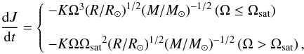$\frac{\mathrm{d}\mathit{J}}{\mathrm{d}\mathit{t}}\mathrm{=}\{\begin{array}{c}\\ \mathrm{-}\mathit{K}{\mathrm{\Omega }}^{\mathrm{3}}{\left(\mathit{R}\mathit{/}{\mathit{R}}_{\mathrm{\odot }}\right)}^{\mathrm{1}\mathit{/}\mathrm{2}}{\left(\mathit{M}\mathit{/}{\mathit{M}}_{\mathrm{\odot }}\right)}^{\mathrm{-}\mathrm{1}\mathit{/}\mathrm{2}}\left(\mathrm{\Omega }\mathrm{\le }{\mathrm{\Omega }}_{\mathrm{sat}}\right)\\ \\ \mathrm{-}\mathit{K}\mathrm{\Omega }{{\mathrm{\Omega }}_{\mathrm{sat}}}^{\mathrm{2}}{\left(\mathit{R}\mathit{/}{\mathit{R}}_{\mathrm{\odot }}\right)}^{\mathrm{1}\mathit{/}\mathrm{2}}{\left(\mathit{M}\mathit{/}{\mathit{M}}_{\mathrm{\odot }}\right)}^{\mathrm{-}\mathrm{1}\mathit{/}\mathrm{2}}\left(\mathrm{\Omega }\mathit{>}{\mathrm{\Omega }}_{\mathrm{sat}}\right)\mathit{,}\end{array}$(1)where the constant K is correlated with the magnetic field strength and is usually taken to be a constant in all stars. Ω_sat is the angular velocity at which saturation occurs, which is adjustable in the model. Following Bouvier et al. (1997), we set K = 2.0 × 10⁴⁷ g   cm²   s and Ω_sat = 14 Ω_⊙.

3.2. Extra mixing in the radiative region

Microscopic diffusion and rotation-induced mixing were considered in the radiative region. The transport of angular momentum and element mixing can be described with two diffusion equations as follows (Chaboyer et al. 1995): $\begin{array}{ccc}\mathit{\rho }{\mathit{r}}^{\mathrm{2}}\frac{\mathit{I}}{\mathit{M}}\frac{\mathrm{d\Omega }}{\mathrm{d}\mathit{t}}& & \mathrm{=}\frac{\mathrm{d}}{\mathrm{d}\mathit{r}}\left(\mathit{\rho }{\mathit{r}}^{\mathrm{2}}\frac{\mathit{I}}{\mathit{M}}{\mathit{D}}_{\mathrm{rot}}\frac{\mathrm{d\Omega }}{\mathrm{d}\mathit{t}}\right)\mathit{,}\\ \mathit{\rho }{\mathit{r}}^{\mathrm{2}}\frac{\mathrm{d}{\mathit{X}}_{\mathit{i}}}{\mathrm{d}\mathit{t}}& & \mathrm{=}\frac{\mathrm{d}}{\mathrm{d}\mathit{r}}\left[\mathit{\rho }{\mathit{r}}^{\mathrm{2}}{\mathit{D}}_{\mathrm{m}\mathit{,}\mathrm{1}}{\mathit{X}}_{\mathit{i}}\mathrm{+}\mathit{\rho }{\mathit{r}}^{\mathrm{2}}\left({\mathit{D}}_{\mathrm{m}\mathit{,}\mathrm{2}}\mathrm{+}{\mathit{f}}_{\mathrm{c}}{\mathit{D}}_{\mathrm{rot}}\right)\frac{\mathrm{d}{\mathit{X}}_{\mathit{i}}}{\mathrm{d}\mathit{t}}\right]\mathit{,}\end{array}$where Ω is angular velocity, X_i is the mass fraction of chemical species i, and I/M is the moment of inertia per unit mass. D_m,1 and D_m,2 are derived from microscopic diffusion coefficients. D_rot is the diffusion coefficient caused by rotation-induced mixing. Details of these three parameters can be found in Chaboyer et al. (1995). The adjustable parameter f_c is used to modify the effects of element mixing caused by rotation. It is determined by requiring that the lithium depletion in the solar model matches the observed depletion (Chaboyer et al. 1995).

In the solar calibration, we adjusted the mixing-length parameter α and the initial helium abundance Y_ini to reproduce the observed solar luminosity and radius at the solar age of 4.57 Gyr. The best solar model evolved with a V_ZAMS of 52.7 km s^-1. When the model reached the solar age, the rotational rate and the lithium abundance were 2.8980 × 10^-6 rad/s and 1.095 dex, respectively, which matched Ω_⊙ = 2.9 × 10^-6 rad/s provided by Bouvier et al. (1997) and log N(Li)_⊙ = 1.10 ± 0.10 dex given in Grevesse & Sauval (1998), and we obtained f_c = 2.95.

4. Results

Our study is based on the four classical features (T_eff, L, [Fe/H] and R) and three additional observed quantities (log N(Li), ${\mathit{P}}_{\mathrm{rot}}^{\mathrm{eq}}$, ⟨△ν⟩ ). The four classical characters T_eff, L, [Fe/H], and R were considered to limit the parameters of 18 Scorpii. Then, two additional observed features (log N(Li), ${\mathit{P}}_{\mathrm{rot}}^{\mathrm{eq}}$) were added in turn as additional constraints. Finally, seismic analyses were carried out to match the observed ⟨△ν⟩ .

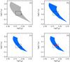Fig. 1 Evolutionary tracks of 18 Scorpii in the H-R diagram constrained by a) the four classical features; b) the classical features + log N(Li); c) the classical features + log N(Li) + ${\mathit{P}}_{\mathrm{rot}}^{\mathrm{eq}}$; d) the blue shadow in the error box represents our estimation based on six nonasteroseismic features. The red shadow in it shows our estimate limited by the pulsation analysis described in Sect. 4.2.

4.1. Stellar parameters determined by nonasteroseismic features

At first, taking into account the four classical features, we obtained nearly 600 tracks, which were considered as candidates for 18 Scorpii. The evolutionary tracks cover the ranges of α from 1.60 to 1.90 and V_ZAMS from 20 to 60 km s^-1. These tracks in the H-R diagram are plotted in gray and are shown in Fig. 1a. The first comparison for 18 Scorpii gave us an estimate of its mass and age of 1.045 ± 0.035 M_⊙ and $\mathrm{3.1}{\mathrm{1}}_{-2.56}^{\mathrm{+}\mathrm{2.08}}$ Gyr, respectively, which is close to that of Meléndez & Ramírez (2007).

The second step was using lithium as a tracer to constrain the mass and age of the star. Lithium is a key element because it is easily destroyed in stellar interiors. Its abundance indicates the amount of internal mixing in the stars and its destruction is strongly mass- and age- dependent (do Nascimento et al. 2009; Li et al. 2012). Among the tracks obtained in the first step, we picked out those fitting the observed lithium abundance log N(Li). We found 101 tracks ranging from 1.70 to 1.90 for α and from 20 km s^-1 to 60 km s^-1 for V_ZAMS. In this way, another estimate of mass and age was obtained, which is $\mathrm{1.03}{\mathrm{0}}_{-0.020}^{\mathrm{+}\mathrm{0.025}} {\mathit{M}}_{\mathrm{\odot }}$ and $\mathrm{3.7}{\mathrm{8}}_{-1.21}^{\mathrm{+}\mathrm{1.45}}$ Gyr, respectively. Moreover, since lithium abundance additionally constraints the range of input parameters, the position of the star in the H-R diagram is restricted to a smaller range than the above, which can be seen in Fig. 1b.

Yet another analysis, considering the observed ${\mathit{P}}_{\mathrm{rot}}^{\mathrm{eq}}$, among the tracks obtained by two above two steps, 18 tracks were found to match the observation, which are plotted in Fig. 1c. The ranges of input parameters α and V_ZAMS were also significantly constrained to 1.70−1.85 and 50−55 km s^-1. The uncertainty of V_ZAMS is reduced in this step. Some of the tracks with improper rotating rate were removed at this step. We plot the rest in Fig. 1c.

4.2. Pulsation analysis

As the final step, we used the stellar pulsation code of Guenther (1994) to preform the seismological analysis for the models by matching all nonasteroseismic features that we obtained in the third step.

The asteroseismic quantity we consider is the mean large separation ⟨△ν⟩ , which is defined as the difference between oscillation modes with the same angular degree and consecutive radial order n: △ν(n) ≡ ν_n,l − ν_n − 1,l. The mean value of the theoretical large separation is calculated from modes with a radial order n ranging from 10 to 25 for l = 0 and 1 modes, and for an order n ranging from 9 to 24 for l = 2 modes, which corresponds to the range 1500−3700 μHz considered in Bazot et al. (2011) when computing the Fourier transform of the spectrum.

Details of all selected models and our results are listed in Table 3. M, Z, α, and V_ZAMS are shown in Cols. 2−5 to describe the initial parameters of the models. Non-asteroseismic properties of the structure models are listed in Cols. 6−12. Column 13 contains the theoretical results of the mean large separation. To constrain the stellar parameters, we considered a 3σ error bar in the mean large separation. In this case, 13 models were found to match the observation. These are shown in Table 3.

After the four steps of our analysis, 13 models were obtained that fit all seven observed features. We used the mean values of their mass, age, effective temperature, luminosity, radius, and surface Z/X as the estimates of stellar parameters. The ranges of the properties of the models provided the corresponding uncertainties. The seismological analysis provided an even better estimate of the mass and age, which is 1.030 ± 0.005 M_⊙ and $\mathrm{3.6}{\mathrm{6}}_{-0.20}^{\mathrm{+}\mathrm{0.14}}$ Gyr, respectively. Additionally, T_eff and L of 18 Scorpii are estimated to be $\mathrm{582}{\mathrm{3}}_{-37}^{\mathrm{+}\mathrm{40}}$ K and 1.067 ± 0.032 L_⊙, respectively. In Fig. 1d, the blue shadow in the error box indicates our estimate based on the six nonasteroseismic properties, the red shadow represents the estimate after the pulsation analysis, which suggests that 18 Scorpii is slightly hotter and brighter than the Sun. The metallicity (Z/X)_s is constrained within $\mathrm{0.023}{\mathrm{8}}_{-0.0001}^{\mathrm{+}\mathrm{0.0002}}$, corresponding to the [Fe/H] of $\mathrm{0.01}{\mathrm{5}}_{-0.002}^{\mathrm{+}\mathrm{0.004}}$. The result indicates that the star has a higher [Fe/H] than the Sun.

4.3. Uncertainty produced by model

The uncertainty of our estimation consists of two parts. One is associated with the observation, which was discussed above. The other is produced by the model and mainly depends on the increment δ of input parameters of our grid calculation described in Table 2. The uncertainty of mass is almost determined by δ of the input mass (± 0.005 M_⊙). The error of the age is more complex. It is firstly associated with the time step set in evolutionary models, which is quite small however, (~0.01 Gyr) and can be ignored. The increments of the other input parameters, i.e., δ of M, Z, α, and V_ZAMS, also influence the uncertainty of the age. We compared the difference between ages of models with adjacent input parameters and similar evolutionary state (for instance, comparing the age of a M = 1.025 M_⊙, Z_ini = 0.0190, α = 1.70 and V_ZAMS = 50 km s^-1 model with that of a M = 1.030 M_⊙, Z_ini = 0.0200, α = 1.75 and V_ZAMS = 55 km s^-1 model when they evolve to similar T_eff and L), and can estimate the error of age produced by the model to be  ~± 0.30 Gyr. In Table 4, we present the two parts of the error separately. Here we obtained the final estimate for 18 Scorpii, which is 1.030 ± 0.010 M_⊙ and $\mathrm{3.6}{\mathrm{6}}_{-0.50}^{\mathrm{+}\mathrm{0.44}}$ Gyr.

4.4. Comparison with previous results

The star 18 Scorpii has previously been studied by several researchers, their methods and estimates are summarized in Table 5. Takeda et al. (2007) and Meléndez & Ramírez (2007) observed this star and provided its mass and age calculated by classical methods. Moreover, do Nascimento et al. (2009) performed a theoretical analysis for 18 Scorpii and obtained its mass and age constrained by lithium abundance. In their work, two different estimates were given (shown in Table 5) based on different observed data. The results inferred a △M ~ 0.006 M_⊙ and a △t ~ 1.0 Gyr. Moreover, Bazot et al. (2011) observed the star for seismology and interferometry, obtaining its average large frequency separation and linear radii. From the homology relation △ν ∝ M^1/2 R^−3/2 (Gough 1994), they suggested the mass of 18 Scorpii to be 1.02 ± 0.03 M_⊙. Very recently, Bazot et al. (2012) obtained another result of an average large frequency separation (133.8 ± 0.2 μHz) of the star, which indicates a mass of 1.01 ± 0.03 M_⊙. Our estimates of mass and age for the star are 1.030 ± 0.010 M_⊙ and $\mathrm{3.6}{\mathrm{6}}_{-0.50}^{\mathrm{+}\mathrm{0.44}}$ Gyr, respectively. The mass determination was close to the results of Takeda et al. (2007), Meléndez & Ramírez (2007), and Bazot et al. (2011) but with higher precision. However, it is more massive than the two results of do Nascimento et al. (2009). Compared with the result of Bazot et al. (2012), our estimate is also more massive because of the difference of average large frequency separation. Our age determination generally agrees within the errors with all previous works. A comparison of mass and age is given in Fig. 2.

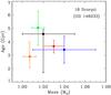Fig. 2 Comparison between mass and age determined in this work (the red error bar) and estimates of previous studies. The black and blue error bars represent the results of Takeda et al. (2007) and Meléndez & Ramírez (2007), respectively. The orange and the green one correspond to the two estimates provided by do Nascimento et al. (2009).

5. Discussion and conclusion

We presented a new application of the do Nascimento et al. (2009) method to improve our knowledge of the physical state of the solar twin star 18 Scorpii (HD 146233, HIP 79672). Based on classical observed features, we used additional observed quantities including lithium abundance and average large frequency separation for better estimates of its stellar parameters.

For solar-type stars, lithium depletes as a function of mass, metallicity, age, and rotational velocity; asteroseismic quantities strongly correlate with the parameters of structure models. Therefore, theoretical analyses of these two additional features can significantly constrain the ranges of the input parameters and ensure a better self-consistent stellar model.

First, estimates of mass and age were calculated with the classical method alone. As we in turn added lithium abundance and the average large frequency separation to our analysis, more accurate determinations were obtained. Finally, an error produced by the model was discussed. After the analysis above, we found the final estimates for mass and age of 18 Scorpii, which are 1.030 ± 0.010 M_⊙ and $\mathrm{3.6}{\mathrm{6}}_{-0.50}^{\mathrm{+}\mathrm{0.44}}$ Gyr, respectively. Moreover, due to the accurate age estimate, we constrained atmospheric features to smaller ranges than the observation. The results locate the star more precisely in the H-R diagram. It allowed us to clarify whether the star has the same observed properties as the Sun.

The rotational history of a star, especially its initial velocity, is difficult to estimate with classical methods. In this work, we found that the possible V_ZAMS of 18 Scorpii is about 55 km s^-1.

The result is close to the solar one (52.7 km s^-1), which was obtained in our solar calibration (see Sect. 3). It means that the star may have experienced a similar rotational evolution as the Sun. The estimate of the initial rotational condition was first determined by the observed ${\mathit{P}}_{\mathrm{rot}}^{\mathrm{eq}}$ and the model of angular momentum evolution. In addition, the interrelation of rotation, lithium depletion, and asteroseismic property also play a role in this question. The change of initial velocity causes a different degree of rotation-mixing in the radiative region, resulting in different processes of lithium depletion (Li et al. 2012). Moreover, rotational mixing also affects the asteroseismic properties of solar-type stars, which has been discussed by Eggenberger et al. (2010). Higher values of the large frequency separation were found for rotating models than for non-rotating ones at the same evolutionary stage in Eggenberger et al. (2010), because rotational mixing increased the effective temperature and to a smaller radius and hence to an increase of the stellar mean density.

18 Scorpii was thought to be a solar twin because of the similar atmospheric parameters to the Sun. In this work, we estimated better stellar parameters for the star by combining the knowledge of lithium depletion, rotating evolution, pulsation analysis and classical method. Our estimates of its atmospheric features, mass, and age suggest that the star is a solar twin slightly more massive and younger than the Sun.

Acknowledgments

This work is supported by grants 10933002 and 11273007 from the National Natural Science Foundation of China, and the Fundamental Research Funds for the Central Universities.

References

All Tables

All Figures

Fig. 1 Evolutionary tracks of 18 Scorpii in the H-R diagram constrained by a) the four classical features; b) the classical features + log N(Li); c) the classical features + log N(Li) + ${\mathit{P}}_{\mathrm{rot}}^{\mathrm{eq}}$; d) the blue shadow in the error box represents our estimation based on six nonasteroseismic features. The red shadow in it shows our estimate limited by the pulsation analysis described in Sect. 4.2.

In the text

	Fig. 2 Comparison between mass and age determined in this work (the red error bar) and estimates of previous studies. The black and blue error bars represent the results of Takeda et al. (2007) and Meléndez & Ramírez (2007), respectively. The orange and the green one correspond to the two estimates provided by do Nascimento et al. (2009).
In the text

References

- Bazot, M., Ireland, M. J., Huber, D., et al. 2011, A&A, 526, L4 [Google Scholar]
- Bazot, M., Campante, T. L., Chaplin, W. J., et al. 2012, A&A, 544, A106 [NASA ADS] [CrossRef] [EDP Sciences] [Google Scholar]
- Bi, S. L., Basu, S., & Li, L. H. 2008, ApJ, 673, 1093 [NASA ADS] [CrossRef] [Google Scholar]
- Bouvier, J., Forestini, M., & Allain, S. 1997, A&A, 326, 1023 [NASA ADS] [Google Scholar]
- Cayrel de Strobel, G., Knowles, N., Hernandez, G., et al. 1981, A&A, 94, 1 [NASA ADS] [Google Scholar]
- Chaboyer, B., Demarque, P., Guenther, D. B., et al. 1995, ApJ, 446, 435 [NASA ADS] [CrossRef] [Google Scholar]
- Castro, M., do Nascimento, J. D., Jr.,Biazzo, K., et al. 2011, A&A, 526, A17 [NASA ADS] [CrossRef] [EDP Sciences] [Google Scholar]
- do Nascimento, J. D., Jr.,Castro, M., Meléndez, J., et al. 2009, A&A, 501, 687 [NASA ADS] [CrossRef] [EDP Sciences] [Google Scholar]
- Eggenberger, P., Meynet, G., Maeder, A., et al. 2010, A&A, 519, A116 [NASA ADS] [CrossRef] [EDP Sciences] [Google Scholar]
- Ferguson, J. W., Alexander, D. R., Allard, F., et al. 2005, ApJ, 623, 585 [NASA ADS] [CrossRef] [Google Scholar]
- Gough, D. O. 1990, in Astrophysics: Recent Progress and Future Possibilities, eds. B. Gustafsson, & P. E. Nissen, 13 [Google Scholar]
- Grevesse, N., & Sauval, A. J. 1998, Space Sci. Rev., 85, 161 [NASA ADS] [CrossRef] [Google Scholar]
- Guenther, D. B. 1994, ApJ, 422, 400 [NASA ADS] [CrossRef] [Google Scholar]
- Guenther, D. B., Demarque, P., Kim, Y. C., & Pinsonneault, M. H. 1992, ApJ, 387, 372 [NASA ADS] [CrossRef] [Google Scholar]
- Kawaler, S. D. 1988, ApJ, 333, 236 [NASA ADS] [CrossRef] [Google Scholar]
- Li, L. H., Basu, S., Sofia, S., et al. 2003, ApJ, 591, 1267 [NASA ADS] [CrossRef] [Google Scholar]
- Li, T. D., Bi, S. L., Chen, Y. Q., et al. 2012, ApJ, 746, 143 [NASA ADS] [CrossRef] [Google Scholar]
- Meléndez, J., & Ramírez, I. 2007, ApJ, 669, L89 [NASA ADS] [CrossRef] [Google Scholar]
- Meléndez, J., Dodds-Eden, K., & Robles, J. A. 2006, ApJ, 641, 133 [NASA ADS] [CrossRef] [Google Scholar]
- Meléndez, J., Asplund, M., Gustafsson, B., et al. 2009, ApJ, 704, 66 [Google Scholar]
- Petit, P., Dintrans, B., Solanki, S. K., et al. 2008, MNRAS, 388, 80 [NASA ADS] [CrossRef] [MathSciNet] [Google Scholar]
- Porto de Mello, G. F., & da Silva, L. 1997, ApJ, 482, 89 [Google Scholar]
- Rogers, F. J., & Nayfonov, A. 2002, ApJ, 576, 1064 [Google Scholar]
- Ramírez, I., Meléndez, J., & Asplund, M. 2009, A&A, 508, 17 [NASA ADS] [CrossRef] [EDP Sciences] [Google Scholar]
- Thoul, A. A., Bahcall, J. N., & Loeb, A. 1994, ApJ, 421, 828 [NASA ADS] [CrossRef] [Google Scholar]
- Takeda, Y., & Tajitsu, A. 2009, PASJ, 61, 471 [NASA ADS] [Google Scholar]
- Takeda, Y., Kawanomoto, S., Honda, S., et al. 2007, A&A, 468, 663 [NASA ADS] [CrossRef] [EDP Sciences] [Google Scholar]
- Valenti, J. A., & Fischer, D. A. 2005, ApJS, 159, 141 [NASA ADS] [CrossRef] [MathSciNet] [Google Scholar]