| Issue |
A&A
Volume 545, September 2012
|
|
|---|---|---|
| Article Number | A123 | |
| Number of page(s) | 3 | |
| Section | Astrophysical processes | |
| DOI | https://doi.org/10.1051/0004-6361/201220228 | |
| Published online | 19 September 2012 | |
Oscillations of the Eddington capture sphere
1 Copernicus Astronomical Center, ul. Bartycka 18, 00-716 Warszawa, Poland
e-mail: This email address is being protected from spambots. You need JavaScript enabled to view it.
2 Institute of Micromechanics and Photonics, ul. św A. Boboli 8, 02-525 Warszawa, Poland
e-mail: This email address is being protected from spambots. You need JavaScript enabled to view it.
3 Physics Department, Gothenburg University, 41296 Göteborg, Sweden
e-mail: This email address is being protected from spambots. You need JavaScript enabled to view it.
; This email address is being protected from spambots. You need JavaScript enabled to view it.
4 Institute of Physics, Faculty of Philosophy and Science, Silesian University in Opava, Bezručovo nám. 13, 74601 Opava, Czech Republic
Received: 14 August 2012
Accepted: 28 August 2012
Abstract
We present a toy model of mildly super-Eddington, optically thin accretion onto a compact star in the Schwarzschild metric, which predicts periodic variations of luminosity when matter is supplied to the system at a constant accretion rate. These are related to the periodic appearance and disappearance of the Eddington capture sphere. In the model the frequency is found to vary inversely with the luminosity. If the input accretion rate varies (strictly) periodically, the luminosity variation is quasi-periodic, and the quality factor is inversely proportional to the relative amplitude of mass accretion fluctuations, with its largest value Q ≈ 1/(10 |δṀ/Ṁ|) attained in oscillations at about 1 to 2 kHz frequencies for a 2 M⊙ star.
Key words: accretion, accretion disks / gravitation / relativistic processes / stars: neutron / X-rays: binaries
© ESO, 2012
1. Introduction
Abramowicz et al. (1990, hereafter AEL) argued that the luminosity of a relativistic star that is accreting at a super-Eddington rate, should periodically change. They have shown that in the combined gravitational and radiation fields of a spherical, compact star, radially moving test particles are captured by a sphere on which the gravitational and radiative forces balance. This is because in Einstein’s general relativity the radiative force diminishes more strongly with the distance than the gravitational force, and radiation may be super-Eddington close to the star, but sub-Eddington further away, reaching the Eddington value at the Eddington capture sphere (ECS), whose radius is given by a simple expression in the Schwarzschild coordinates (Phinney 1987), 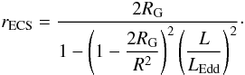 (1)Here R is the radius of the star, RG = GM/c2 its gravitational radius, and L, which is assumed to satisfy Eq. (2), is the stellar luminosity at its surface. Bini et al. (2009); Oh et al. (2011), and Stahl et al. (2012) have shown that the ECS captures particles from a wide class of non-radial orbits as well1, so the following discussion is not restricted to the case of radial accretion. However, it is important to keep in mind that the balance of forces necessary for the existence of the ECS requires a large, radial radiative flux. In non-spherical accretion this can only be realized in the optically thin regime.
In this paper we present a simple model in which the idea of periodic luminosity changes is realized. AEL assumed that the radiation power was provided by the kinetic energy of the accreted particles, released when they hit the surface of the star. As stressed by Stahl et al. (2012), particles settle on the ECS rather gently, so the ECS itself is not particularly luminous. If all particles are captured at the Eddington sphere, they do not reach the surface of the star, and the stellar accretion luminosity goes to zero. When it does, and actually already when L/LEdd < (1−2RG/R)−1/2, the ECS disappears, accretion is resumed by the star and eventually the luminosity may build up to its former value, so the ECS will reappear and accretion will stop again. Thus, the accretion process may be quasiperiodic, alternating between states of high luminosity and no luminosity.
2. The model
The toy model considered here assumes a steady2 supply of optically thin fluid at some distance above the stellar surface. As shown by Stahl et al. (2012), unless its velocity is extraordinarily large the fluid will settle on the ECS, regardless of its point of origin, if only  (2)In our model the stellar luminosity will be assumed to be either zero, or to have a certain definite value, L = L0, satisfying Eq. (2). In this sense the model states are binary (on-off). This property implies that the ECS is located at a specific radius, rECS = r0 > R, whenever present (Eq. (1)). The model is described by three equations:
 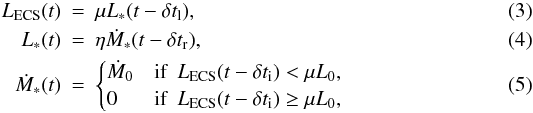 where LECS is the stellar luminosity at the ECS, L ∗ is the luminosity at the stellar surface, Ṁ ∗ is the accretion rate at the stellar surface, μ is a redshift factor between R and r0, η is the conversion factor between accretion rate and stellar luminosity.
The simplest possibility, which we will ignore, is that ηṀ0 < LEdd(1−2RG/R)−1/2, so the critical luminosity for establishing the ECS is never reached, and the equations describe a steady state solution. We will assume instead that L0 = ηṀ0, i.e., the stellar luminosity in the “on” state has the necessary value to establish an ECS at the radius r0. This assumption allows non-trivial time behaviour of the model system.
There are three timescales that determine the behaviour of the model, the reaction time δtr, which is the timescale for converting accreting matter into radiation, the light travel time δtl, which is the travel time of light from the stellar surface to the ECS, and the infall time δti, which is the infall time of matter from the ECS to the stellar surface in the absence of radiation. Now, δtl and δti can be determined from RG,R and r0. So, for a given star these two timescales are a function of the stellar luminosity alone, i.e., of ηṀ0. The reaction time introduces a phase shift between accretion and radiation at the stellar surface. In numerical examples we will adopt two extreme values δtr = 0, or δtr = 0.1 ms, the latter being the estimated cooling time of a clump of fluid that falls on a neutron star surface (Kluźniak et al. 1990).
In reality, the time delays would not be as sharp as we have assumed them to be. For instance, even at time δtl after the luminosity is turned off, particles outside the ECS suffer from radiation drag for an additional interval of time (r − r0)/c, where r is the position of the particle at time δtl + (r − r0)/c after the radiation is turned off. Conversely, after the luminosity is turned on again, all particles between the ECS and the stellar surface will feel the full impact of radiation pressure after a delay of only (r − R)/c < δtl, where again, r is the position of the particle when the radiation front passes it, (r − R)/c after the radiation is turned on. In the toy model, we neglect such effects entirely.
Combining Eqs. (3)–(5) we find that Ṁ∗(t) is determined by Ṁ∗(t − T), with T = δti + δtr + δtl: 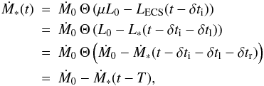 where Θ is the Heaviside step function. Thus,
 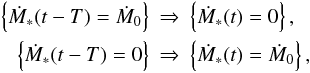 and clearly, the model system shows periodic behaviour with the period 2T:
  (6)
(6)
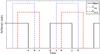 |
Fig. 1 Stellar accretion rate and luminosities at the stellar surface and at the ECS, according to the model. |
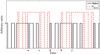 |
Fig. 2 Stellar accretion rate and the luminosity at the ECS, for another choice of initial conditions. |
3. Results of the model
A typical behaviour of the model is shown in Fig. 1 which shows a solution of Eqs. (3) − (5) with δtl:δti:δtr = 8:17:10. The black solid line traces Ṁ∗. In the figure, we identify the time b − a = e − d = δtr as the reaction time, c − b = h − e = δtl as the light travel time, and d − c = j − h = δti as the infall time. The luminosities at the stellar surface and at the ECS are shifted relative to the accretion rate by δtr and δtr + δtl, respectively. We note also that d − a = j − d = h − c = k − e = e − b = δtr + δtl + δti = T, and the pulses are as long as the periods without activity. Thus the period of the oscillation is P = 2T, as expected from Eq. (6).
In constructing Fig. 1 it was assumed that matter first arrives at the stellar surface at t = 0 and that there is a continual inflow of matter to the system at the rate Ṁ0 for all t ≥ 0. Different initial conditions can lead to a more complicated pulse shape of Ṁ∗(t) for t in the intervals (2nT,2nT + T), with its complement Ṁ∗(t) = Ṁ0 − Ṁ∗(t − T) in the intervals (2nT + T,2nT + 2T). Here, and elsewhere, n = 0,1,2,3 .... The state of accretion (Ṁ0 or 0) at time t has no influence on the future value of Ṁ∗ until the time t + T, so one can assume that at any instant in the initial interval t ∈ [0,T) the accretion rate has any of the two values, 0 or Ṁ0, i.e., in this interval Ṁ∗(t) = Ṁ0g(t), where g(t) is an arbitrary binary function, mapping the initial time interval into on-off states, g: [0,T) → { 0,1 } . Figure 2 provides an example of such behaviour. Thus, in principle, the harmonic content of the signal may be quite rich, although the fundamental is still at f = 1/P = 1/(2T).
As can be seen from Eqs. (3)–(5) the model takes no account of accumulation of matter on the ECS, that is to say, here we ignore the arrival at t = 2(n + 1)T (and at other moments as well in the case of Fig. 2), of the additional matter that had accumulated on the ECS. In reality, this matter would produce a brief flash of radiation of energy ηECSṀ0ΔT, where ηECS is the conversion efficiency to radiation of the kinetic energy of matter falling from the ECS, and ΔT is the accumulation time (ΔT = T in Fig. 1). If in the steady accretion phase matter is falling in from r ≫ r0, one would expect ηECS ≪ η.
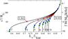 |
Fig. 3 The semi-period T of the oscillation in geometrical units as a function of peak luminosity at infinity in Eddington units, when kinetic energy is instantaneously converted to luminosity (δtr = 0). The corresponding frequency f = 1/(2T) can be read off in kHz from the right vertical axis. The curves are labeled with the stellar radius (3, ...,10) in units of RG. Filled squares indicate a value of the slope dlog T/dlog L∞ = 50, filled circles a value of 100, and the crosses the minimum value of the logarithmic derivative for each curve. |
In a physically realistic situation the infall time is the dominant time scale, δti ≫ δtl. The radius of the ECS, and hence also the infall time, increases rapidly with L∞, and without bounds as L∞ → LEdd: ![Mathematical equation: \begin{equation} \label{ECS} \frac{r_{\rm ECS}}{2R_{\rm G}} = {\left[1 - \left(\dfrac{L_\infty}{L_{\rm Edd}} \right)^2\right]^{-1}}\cdot \end{equation}](/articles/aa/full_html/2012/09/aa20228-12/aa20228-12-eq80.png) (7)Here, L∞ is the redshifted luminosity at infinity. Hence, except for the lowest values of the luminosity parameter L0, the infall time δti is the dominant time scale, and the frequency of oscillations f = 1/(2T) varies inversely with the luminosity. Neglecting δtr, we can compute the semi-period T, and the frequency of oscillation as a function of the stellar radius R and of the luminosity L∞ alone-T and f will, respectively, scale directly or inversely with M. These are shown in Fig. 3 for various stellar radii. Figure 4 shows the frequency as a function of luminosity, for a star with M = 2 M⊙, when δtr = 0.1 ms.
(7)Here, L∞ is the redshifted luminosity at infinity. Hence, except for the lowest values of the luminosity parameter L0, the infall time δti is the dominant time scale, and the frequency of oscillations f = 1/(2T) varies inversely with the luminosity. Neglecting δtr, we can compute the semi-period T, and the frequency of oscillation as a function of the stellar radius R and of the luminosity L∞ alone-T and f will, respectively, scale directly or inversely with M. These are shown in Fig. 3 for various stellar radii. Figure 4 shows the frequency as a function of luminosity, for a star with M = 2 M⊙, when δtr = 0.1 ms.
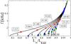 |
Fig. 4 The frequency of the oscillations as a function of peak luminosity at infinity in Eddington units, when there is a delay in converting kinetic energy to luminosity δtr = 0.1 ms (see Kluźniak et al. 1990). The stellar mass is assumed to be M = 2 M⊙. The curves are labeled with the stellar radius (3, ...,10) in units of RG. Filled squares indicate a value of the slope dlog T/dlog L∞ = 30, filled circles a value of 50, and the crosses the minimum value of the slope for each curve (boxed values). |
4. Conclusions and discussion
We have shown that supplying mass to the vicinity of a compact star, continuously and at a constant accretion rate, can lead to periodic top-hat variations of luminosity, if only the mass accretion rate corresponds to a mildly super-Eddington luminosity at the stellar surface. This oscillatory behaviour of luminosity is related to the phenomenon of the ECS, which is a consequence of the interplay of radiation drag and general relativity.
If such an oscillation occurs in the real world, for example in the Z sources, where rapid variations of the inferred inner radius of the accretion disk have been reported (Lin et al. 2009), the actual mechanism is likely to be more complex than the strictly periodic oscillation in the toy model considered here. E.g., the accretion rate is not likely to be constant (contrary to our assumption of simple on-off behaviour at the stellar surface).
As a minor extension of the model, consider an accretion rate that is varying on a timescale comparable to the period of the ECS oscillator. Even strictly periodic variation of Ṁ0 will lead to a decoherence of the ECS oscillation, because the position r0 of the ECS and (hence) the infall time from the ECS, and (hence) the oscillator frequency, are strongly varying functions of the luminosity, L0 = ηM0. Indeed, 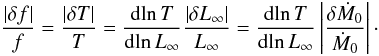 (8)Thus, the Q factor of the oscillation is
 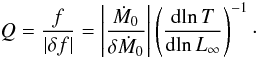 (9)We have indicated some values of the logarithmic derivative dlnT/dlnL∞ in Figs. 3, 4. Comparing the figures, we see that delayed emission (reaction time δtr > 0) at the stellar surface acts as a low-pass filter, cutting out the highest frequencies. At the same time it improves the quality factor of the oscillator.
Accreting neutrons stars in low mass X-ray binaries are expected to have a radius in the range of 4 to 7GM/c2 (Arnett & Bowers 1977; Kluźniak & Wagoner 1985), and a mass of about two solar masses. It is seen from Fig. 4 that the minimum values of the logarithmic derivative attained for radii of 4, 5, 6, 7GM/c2 are between 5 and 15. Hence, the maximum expected value of the oscillator quality factor would be Q ≈ 1/(10 | δṀ0/Ṁ0 | ), occurring for frequencies between about 1 and 2 kHz, as can be seen from Fig. 4.
As shown in detail by Oh et al. (2011), azimuthal radiation drag efficiently removes particle’s angular momentum, typically making motions in the combined gravitational and radiation fields asymptotically radial.
The assumption of a constant Ṁ will be relaxed in Sect. 4.
Acknowledgments
Research supported in part by Polish NCN grants UMO-2011/01/B/ST9/05439 and N N203 511238.
References
- Abramowicz, M.A., Ellis, G. F. R., & Lanza, A. 1990, ApJ, 361, 470 [NASA ADS] [CrossRef] [Google Scholar]
- Arnett, W. D., & Bowers, R. L. 1977, ApJS, 33, 415 [NASA ADS] [CrossRef] [Google Scholar]
- Bini, D., Jantzen, R. T., & Stella, L. 2009, Class. Q. Grav., 26, 055009 [Google Scholar]
- Kluźniak, W., & Wagoner, R. V. 1985, ApJ, 297, 548 [NASA ADS] [CrossRef] [Google Scholar]
- Kluźniak, W., Michelson, P., & Wagoner, R. V. 1990, ApJ, 358, 538 [NASA ADS] [CrossRef] [Google Scholar]
- Lin, D., Remillard, R. A., & Homan, J. 2009, ApJ, 696, 1257 [NASA ADS] [CrossRef] [Google Scholar]
- Oh, J. S., Hongsu, J., & Hyung, M. L. 2011, New Astron., 16, 183 [NASA ADS] [CrossRef] [Google Scholar]
- Phinney, E. S. 1987, in Superluminal Radio Sources, eds. J. A. Zensus, & T. J. Pearson (Cambridge: Cambridge University Press), 12 [Google Scholar]
- Stahl, A., Wielgus, M., Abramowicz, M. A., Kluźniak W., & Yu, W. 2012, A&A, in press, DOI: 10.1051/0004-6361/201220187 [Google Scholar]
All Figures
|
Fig. 1 Stellar accretion rate and luminosities at the stellar surface and at the ECS, according to the model. |
| In the text | |
|
Fig. 2 Stellar accretion rate and the luminosity at the ECS, for another choice of initial conditions. |
| In the text | |
|
Fig. 3 The semi-period T of the oscillation in geometrical units as a function of peak luminosity at infinity in Eddington units, when kinetic energy is instantaneously converted to luminosity (δtr = 0). The corresponding frequency f = 1/(2T) can be read off in kHz from the right vertical axis. The curves are labeled with the stellar radius (3, ...,10) in units of RG. Filled squares indicate a value of the slope dlog T/dlog L∞ = 50, filled circles a value of 100, and the crosses the minimum value of the logarithmic derivative for each curve. |
| In the text | |
|
Fig. 4 The frequency of the oscillations as a function of peak luminosity at infinity in Eddington units, when there is a delay in converting kinetic energy to luminosity δtr = 0.1 ms (see Kluźniak et al. 1990). The stellar mass is assumed to be M = 2 M⊙. The curves are labeled with the stellar radius (3, ...,10) in units of RG. Filled squares indicate a value of the slope dlog T/dlog L∞ = 30, filled circles a value of 50, and the crosses the minimum value of the slope for each curve (boxed values). |
| In the text | |
Current usage metrics show cumulative count of Article Views (full-text article views including HTML views, PDF and ePub downloads, according to the available data) and Abstracts Views on Vision4Press platform.
Data correspond to usage on the plateform after 2015. The current usage metrics is available 48-96 hours after online publication and is updated daily on week days.
Initial download of the metrics may take a while.