| Issue |
A&A
Volume 545, September 2012
|
|
|---|---|---|
| Article Number | A86 | |
| Number of page(s) | 10 | |
| Section | Interstellar and circumstellar matter | |
| DOI | https://doi.org/10.1051/0004-6361/201218938 | |
| Published online | 12 September 2012 | |
Radio perspectives on the Monoceros SNR G205.5+0.5
National Astronomical Observatories, Chinese Academy of
Sciences,
Jia-20, Datun Road, Chaoyang District,
100012
Beijing,
PR China
e-mail: xl@nao.cas.cn; mz@nao.cas.cn
Received:
1
February
2012
Accepted:
27
July
2012
Context. The Monoceros supernova remnant (SNR G205.5+0.5) is a large shell-type SNR located in the Rosette molecular complex and thought to be interacting with the Rosette Nebula.
Aims. We aim to re-examine the radio spectral index and its spatial variation over the Monoceros SNR as well as study its properties of evolution within the complex interstellar medium.
Methods. We extracted radio continuum data for the Monoceros complex region from the Effelsberg 21 cm and 11 cm surveys and the Urumqi 6 cm polarization survey. We used the new Arecibo GALFA-HI survey data with much higher resolution and sensitivity than that previously available to identify the HI shell related with the SNR. Multi-wavelengths data are included to investigate the properties of the SNR.
Results. The spectral index α (Sν ∝ να) averaged over the SNR is −0.41 ± 0.16. The TT-plots and the distribution of α over the SNR show spatial variations that steepen toward the inner western filamentary shell. Polarized emission is prominent on the western filamentary shell region. The RM there is estimated to be about 30 ± 77n rad m-2, where the n = 1 solution is preferred, and the magnetic field has a strength of about 9.5 μG. From the HI channel maps, further evidence is provided for an interaction between the Monoceros SNR and the Rosette Nebula. We identify partial neutral hydrogen shell structures in the northwestern region at velocities of +15 km s-1 circumscribing the continuum emission. The HI shell has swept up a mass of about 4000 M⊙ for a distance of 1.6 kpc. The western HI shell, well associated with the dust emission, is found to lie outside of the radio shell. We suggest that the Monoceros SNR is evolving within a cavity blown out by the progenitor and has triggered part of the star formation in the Rosette Nebula.
Conclusions. The Monoceros SNR is interacting with the ambient interstellar medium with ultra-high energy emission detected. Its interaction with the Rosette Nebula is further supported by new evidence from HI data, which will help the investigation of the emission mechanism of the high-energy emission.
Key words: ISM: supernova remnants / polarization / radio continuum: general / methods: observational
© ESO, 2012
1. Introduction
The Monoceros SNR is an extended filamentary object lying in the anti-center complex region. The bright Rosette Nebula (SH 2-275) and HII region SH 2-273 are adjacent to the edge of the southern and northeastern shell of the supernova remnant (SNR). It was first recognized as a possible supernova remnant by Davies (1963) from radio observations at 237 MHz. More detailed observations presented by Holden (1968) confirmed this property by a nonthermal radio spectrum.
The SNR has been studied at low and intermediate radio frequencies by Holden (1968), Milne & Hill (1969), and Dickel & Denoyer (1975). Observations at frequencies near 2700 MHz were made by Day et al. (1972); Milne & Dickel (1974); Velusamy & Kundu (1974); Graham et al. (1982). Graham et al. (1982) found an average spectral index α = −0.47 ± 0.06 from 111−2700 MHz radio data. In addition, they presented the spatial spectral index distribution at 178−2700 MHz and 611−2700 MHz, which was found to be steeper in the inner region. In addition, they identified an HII region (G206.35+1.35) in the eastern periphery from its thermal spectrum. Gao et al. (2011) showed a new polarization observation at 4800 MHz. Combining this observation with Effelsberg 21 cm and 11 cm data, they obtained a spectral index of α = −0.43 ± 0.12 for the western shell. Early 11 cm polarization observations were made by Milne & Dickel (1974), but no significant polarized emission was detected. The 6 cm polarization map showed that the magnetic field is closely aligned with the filamentary shell.
The distance to the Monoceros SNR has been estimated to range from around 800 pc to about 1.6 kpc. Odegard (1986) summarized all the available evidence and argued that the Monoceros SNR is at the same distance as the Monoceros OB2 association of about 1.6 kpc. This is further supported by the decimeter observations of the absorption of nonthermal emission from the supernova remnant by the Rosette Nebula (Odegard 1986). The diameter of the SNR is then about 106 pc (3.8°), and the age is about 1.5 × 10⁵ yr. A study of Einstein IPC data (Leahy et al. 1985, 1986) shows diffuse X-ray emission from the Monoceros SNR shock front, corresponding to the optical filaments. By fitting the data, they concluded that the SNR was expanding in a low-density (0.003 cm-3) medium and had not yet entered the radiative phase (Leahy et al. 1986). Riddle (1972) identified a neutral hydrogen shell located outside of the Monoceros optical filament with low-resolution HI data.
It has been suggested that the Monoceros SNR interacts with the Rosette Nebulae. In the SNR ridges overlapping the Rosette region, Fountain et al. (1979) found broadened line widths of H109α and more enhanced than average Hα emission in the Rosette Nebula. EGRET detected extended γ-ray emission (3EG J0634+0521) from the region associated with the Monoceros/Rosette Nebula in the energy range from 100 MeV up to 10 GeV (Jaffe et al. 1997). This emission was interpreted as γ-rays from the decay of π0’s produced by the interaction of shock-accelerated protons with the ambient matter. HESS found a source HESS J0632+057 (100 GeV−10 TeV) located at the rim of the western SNR shell (Fiasson et al. 2008), which seems to be related with 3EG J0634+0521 and an associated molecular cloud. An observation carried out with the BeppoSAX satellite (Kaaret et al. 1999) discovered a hard spectrum X-ray point source (SAX J0635+0533) within the 95% probability circle of the EGRET detection, which was later identified as a binary pulsar (Cusumano et al. 2000). Torres et al. (2003) postulated that both the binary pulsar SAX J0635+0533 and the emission from the interaction region between the expanding shell and the Rosette Nebula contribute to the EGRET γ-ray emission.
Although there is already a considerable body of radio observations on the Monoceros SNR, we try to better delineate the extent of the SNR and the spatial spectral index variations using new radio data with higher resolution. Also, a new high-sensitivity, high-resolution HI data cube enables us to identify HI features morphologically associated with the SNR and to discuss various evolutionary scenarios. In Sect. 2, we describe the 11, 21, and 6 cm radio continuum observations, as well as the HI data of the Monoceros SNR. The determination of the flux densities and the spectral index distribution are presented in Sect. 3. The polarization properties and the magnetic fields in the northeast filamentary shell are estimated in Sect. 4, while the associated HI shell analysis is presented in Sect. 5. Finally, we give a discussion and summary in Sects. 6 and 7, respectively.
2. Data
2.1. Radio data
The 21 cm and 11 cm radio continuum data presented here are taken from the Effelsberg Galactic plane survey (Reich et al. 1990; Fürst et al. 1990). The angular resolutions of these surveys are 9.4′ and 4.4′, respectively. The 6 cm continuum and polarization data are extracted from the Sino-German polarization survey of the Galactic plane (Gao et al. 2010) made with the Urumqi 25 m telescope. The angular resolution is 9.5′ at 4.8 GHz. Detailed system and observation parameters and the data reduction procedure are described in these related papers.
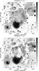 |
Fig. 1 Effelsberg 21 cm and 11 cm continuum images of the Monoceros SNR, with angular resolutions of 9.4′ and 4.4′ respectively. Contours at 21 cm start from 100 mK TB and increase by 2n × 80 mK TB (n = 0,1,2,3,...). Contours at 11 cm are drawn according to 2n × 30 mK TB, with n = 0,1,2,3,... |
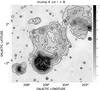 |
Fig. 2 Urumqi 6 cm total intensity map of the Monoceros SNR at an angular resolution of 9.5′. Polarization vectors in the B-field direction (E+90°) are overlaid. The length of the bars is proportional to PI, with a polarized intensity of 1 mK TB, corresponding to a bar-length of 2′. Total intensity contours are drawn according to 2n × 10 mK TB, with n = 0,1,2,3,... |
Figure 1 shows the Effelsberg 21 cm and 11 cm total
intensity images of the Monoceros SNR. The Urumqi 6 cm continuum emission with
corresponding polarization intensity (E-vectors) overlaid are presented in Fig. 2. Filamentary shell structures are clearly seen in the
northern, western, and southern regions, with diffuse emission in the eastern portion. The
HII region 0641+06 ( ) was identified by Graham et al. (1982). There is also a small emission
ridge (
) was identified by Graham et al. (1982). There is also a small emission
ridge ( ) projecting from the Rosette
Nebula toward the east. In Sects. 3 and 5, we propose this structure to be part of the
Monoceros southern shell.
) projecting from the Rosette
Nebula toward the east. In Sects. 3 and 5, we propose this structure to be part of the
Monoceros southern shell.
2.2. HI data
The HI data sets come from the recently released Galactic Arecibo L-Band Feed Array HI survey (GALFA-HI), described in detail by Peek et al. (2011). The angular resolution of the survey is about 4′. It covers a wide velocity range from −700 km s-1 to +700 km s-1, with a velocity resolution of 0.18 km s-1. Typical noise levels are 80 mK in an integrated 1 km s-1 channel.
3. Spectral index analysis
3.1. Subtracting the thermal radio continuum emission
Thermal emission is well traced by the infrared (IR) emission from the dust. We present
the IRIS 60 μm image of the Monoceros complex region in Fig. 3. The IR observations are the high-resolution
reprocessed IRAS image produced at the Infrared Processing and Analysis Center (IPAC;
Miville-Deschênes & Lagache 2005).
Besides the strong thermal emission from the Rosette Nebula, there is a thermal source
( ) within the SNR region and
HII region 0641+06 within the shell.
) within the SNR region and
HII region 0641+06 within the shell.
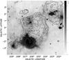 |
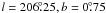
Fig. 3 IRIS 60 μm emission of the same area as in the preceding radio continuum images. Resolution is 2′. Contours of 6 cm total intensity are overlaid and have the same levels as for Fig. 2. |
We tried to separate and subtract the aforementioned thermal sources using the correlation between the radio brightness temperature and its equivalent dust flux at 60 μm (e.g., Broadbent et al. 1989; Fürst et al. 1987). This correlation generally exists for diffuse thermal emission and has been used to remove the thermal background emission from SNRs.
For diffuse HII regions, Broadbent et al. (1989) obtained the relation TB,11 = (6.4 ± 1.7) × I60, where TB,11 is in mK and I60 in MJy sr-1. Assuming a temperature spectral index β = −2.10, the corresponding relation at 21 cm becomes TB,21 = 24.6I60. We made a TT-plot between 21 cm and 6 cm for the thermal source region. A temperature spectral index β = −2.10 ± 0.22 confirms the thermal nature of the emission. We convolved the 21 cm and 60 μm images to the same 10′ resolution and plotted the brightness at 60 μm (I60) against that at 21 cm (TB,21). The resulting correlation is shown in Fig. 4, from which we find a slope of 23.6 mK MJy-1 sr, comparable with the theoretical value. We were then able to estimate the theoretical thermal emission and simply subtract it from the raw images. The thermal emission at 11 cm and 6 cm is simply interpolated using a spectral index of β = −2.10.
We checked the similar relation for the Rosette Nebula. Both the Effelsberg 21 cm total intensity data and the IRIS 60 μm data were convolved to 10′ and scaled to units of Jy/beam. The ratio TB,21/I60 shows large scatter in the periphery, with an average value of about 90 mK MJy-1 sr in the central region. In regions where the two objects overlap each other, it is difficult to separate the nonthermal emission from the SNR and the thermal emission from the Rosette Nebula. Therefore, we directly exclude the Rosette Nebula emission by setting a boundary in between to obtain the emission from the SNR alone.
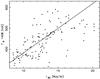 |
Fig. 4 Plot of the brightness temperature TB,21 against the brightness I60. The best-fit straight line corresponds to a slope of 23.6 mK MJy-1 sr. |
3.2. Integrated flux densities and TT-plots
In order to estimate integrated flux densities and derive an accurate spectral index for the remnant, we removed by Gaussian fitting five bright point-like sources from the 21, 11, and 6 cm total intensity maps within the area of the Monoceros SNR.
We used the method of temperature-versus-temperature plots (TT-plots; Turtle et al. 1962) to adjust the base levels for the entire SNR area at two wavelengths. Both maps were convolved to a common angular resolution of 10′. Corresponding to the TT-plot results for the entire shell region, we found a constant offset of 3 mK TB at 6 cm, 55 mK TB at 11 cm, and about 35 mK TB at 21 cm.
The integrated flux densities were obtained by setting polygons just outside the periphery of the SNR and integrating the enclosed emission. The contribution of the Rosette Nebula was excluded by setting the highest brightness temperature in the shell as its boundary. From variations outside the SNR, we estimated a remaining uncertainty in setting the base level of 9.9 mK TB at 21 cm, 7.9 mK TB at 11 cm, and 3.5 mK TB at 6 cm. We obtained a flux density of 120.8 ± 9.9 Jy for the Monoceros SNR at 21 cm, 89.7 ± 7.9 Jy at 11 cm, and 73.4 ± 3.5 Jy at 6 cm. The linear fit to these integrated flux densities for the Monoceros SNR is shown in Fig. 5, yielding a spectral index of α = −0.41 ± 0.16.
The TT-plot method is unaffected by the uncertainty of the background levels in the maps. We also applied it to an investigation of the spectral index for different sections of the Monoceros SNR shell. The temperature spectral index β (β = α − 2) found from fitting the slope of 21 cm and 6 cm pairs of different shell regions is shown in Fig. 6. The error of β for the diffuse eastern shell is relatively large, probably due both to its low brightness and confusion with weak unresolved background sources that could not be subtracted. We also investigated the southern shell region, which is mixed with the Rosette Nebula. In addition to the old spherical shell region, there is a new shell-like feature protruding out toward the east (see Sect. 2.1). The index of this new feature is about α = −0.53 ± 0.44. The large uncertainty is due to the weak emission, plus the residuals after a point-source has been subtracted. However, the spectral-index distribution in this region in Fig. 4 of Graham et al. (1982), as well as Fig. 7 in Sect. 3.3, is compatible with the feature being nonthermal. It seems that this feature is likely to be a part of the Monoceros SNR.
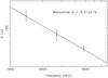 |
Fig. 5 Spectral index from integrated flux densities of the Monoceros SNR. |
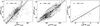 |
Fig. 6 TT-plots between Urumqi 6 cm data and the Effelsberg 21 cm data (as examples) for the eastern shell, northwest filamentary shell, and newly identified southern branch shell of the Monoceros SNR. |
3.3. Spectral index map
We calculated the spectral index for each pixel of the Monoceros SNR from the zero-level corrected images at the three frequencies by linearly fitting for intensities versus frequencies using a logarithmic scale. In order to achieve reasonable spectral indices without significant influence from noise or local distortions, a lower intensity limit of 180 mK TB, 30 mK TB, and 6 mK TB is set for the 21, 11, and 6 cm maps, respectively. The regions outside the remnant are blanked out. We display the temperature spectral index map from 21, 11, and 6 cm in Fig. 7. Possible remaining variations of the base levels at 11 cm or 6 cm yield an average systematic uncertainty of the spectral indices of Δα ~ 0.2, with errors being larger in regions of weak emission.
The Rosette Nebula shows a flat brightness spectral index, as expected for optically thin
thermal emission from an HII region. The spectral index of the SNR G206.9+2.3 presents
fairly uniform distribution and has an averaged index of β = −2.46,
similar to the value found for its integrated flux densities by Gao et al. (2011). Spectral index values are generally about −0.4 in
the Monoceros SNR shell region. The new shell-like feature in the southern shell has an
index of about −0.5. Little significant spectral variation is traced in the overlap
region with the Rosette Nebula. The spectral index gets steeper in the inner region, so
that the inner western filament at  has a steeper spectral
index of about −0.6. The value is generally consistent with that in the lower frequency
spectral index map between 178 and 2700 MHz (Graham et al.
1982).
has a steeper spectral
index of about −0.6. The value is generally consistent with that in the lower frequency
spectral index map between 178 and 2700 MHz (Graham et al.
1982).
Graham et al. (1982) excluded the possibility that the difference comes from a mixture of thermal emission for the more northerly rim of NGC 2264 by using a positional argument and comparing with the lower frequency index. The new higher frequency 6 cm data further excludes this possibility. The relativistic electrons in the inner western ridge probably have a different energy spectrum, as proposed by Graham et al. (1982). It is now generally accepted that relativistic electrons responsible for the synchrotron emission are produced by the Fermi acceleration mechanism (Bell 1978a,b). This process predicts a spectral index given by −β = 2 + (M2 + 3)/ [2(M2−1)] , where M is the Mach number of the shock. For a very strong shock, M is close to three, corresponding to an average value of β = −2.75. A weaker shock produces a steeper spectrum. The shock in the inner western filament is possibly weaker with a decreased compression ratio and results in a steeper spectrum. In addition, a steeper spectrum could also have originated from high-energy electrons due to synchrotron aging, when propagating in a weak magnetic field region. However, the strength of the magnetic field in both western ridges appears to be similar from the vectors in the 6 cm map, both from the perpendicular component B⊥ and the amounts of Faraday rotation. No indication of a spectral break is found in the frequency range from 178 MHz to 4.8 GHz, which means that any spectral break due to synchrotron aging should be at higher frequencies. Higher frequency data are needed to distinguish between these two explanations.
4. Polarization analysis
4.1. The linear polarization properties
The 6 cm polarization map is shown in Fig. 2. Prominent polarized emission is mainly displayed toward the western shell of the SNR. The observed magnetic vectors are distributed almost along the ridges of the two branches. This indicates a well-ordered magnetic field in the shell, as expected for an evolved SNR (Fürst & Reich 2004). The polarization percentage of the inner filament is about 20% at 6 cm and less at about 10% in the outer filament. Except for the enhanced polarization along the SNR’s western shell, polarized emission in other shell regions is very weak. The inner polarization patch might originate from polarized diffuse interstellar emission, possibly mixed with polarized emission from the SNR of about similar strength. Strongly polarized emission is also detected from the SNR G206.9+2.3.
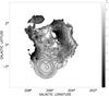 |
Fig. 7 Temperature spectral index map of the Monoceros SNR from 21/11/6 cm maps. Regions where the random error exceeds 0.06 have been blanked out. Contours of 6 cm total intensity with the same levels as Fig. 2 are overlaid. |
The large-scale emission component is missing in the 6 cm polarization map, due to the zero-level setting during observation and data analysis. This is known to limit the interpretation of polarization structures caused by Faraday effects in the interstellar medium (Reich 2006), except in strongly polarized regions. We checked the polarization map with large-scale polarized emission added, which is extrapolated from the WMAP K-band data using an appropriate spectral index (see Fig. 6 in Gao et al. 2010). Strongly polarized emission from the diffuse interstellar medium appears near the Galactic plane. The polarized signal from the western shell of the Monoceros SNR is sufficiently strong that it remains almost unchanged by adding the large-scale emission component.
We extracted the 21 cm polarized intensity map of the same region (Fig. 8) from the polarization survey made with the DRAO 26-m telescope (Wolleben et al. 2006). This map includes the large-scale polarized emission component at an absolute zero level with an angular resolution of 36′. We found a large diffuse interstellar polarization patch covering the Monoceros SNR region, with enhanced polarized emission coinciding with the western filamentary shell region. The polarization angles in the western shell lie nearly perpendicular to the shell. Polarized emission from a larger distance might have been depolarized toward the Rosette Nebula, where weakly polarized emission is detected at 21 cm.
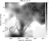 |
Fig. 8 DRAO 21 cm polarized intensity map of the Monoceros SNR at an angular resolution of 36′. Polarization vectors in the B-field direction (E+90°) are overlaid. The length of the vectors is proportional to PI. A polarized intensity of 1 mK TB corresponds to a length of 0.05′. Contours show total intensities starting at 200 mK TB and increasing by 2n × 60 mK TB (n = 0,1,2,3,...). The positions of RM sources in Taylor et al. (2009) are indicated by crosses, with lengths proportional to the RM values. |
Compared to the western shell, the low polarization percentage of the eastern shell indicates a more irregular magnetic field. The background polarization there is depolarized by small-scale magneto-ionic fluctuations in the shell and/or polarized emission from the SNR shell with a different orientation. In the southern shell where interaction has occurred, as discussed in Sect. 5.3, high-thermal electron densities in the Rosette Nebula (Odegard 1986) and their fluctuations could be sufficiently strong to cause a heavy depolarization of the background polarization.
4.2. Rotation measures of the western shell
Since the polarized emission from the western shell is strong and clearly stands out against the background in the 21 cm polarization map, we were able to remove the diffuse Galactic polarized emission component and calculate the rotation measure (RM) distribution using the polarization angles from the 21 and 6 cm polarization maps. We subtracted an average value of 81 mK TB from the 21 cm U map and “twisted” the Q map by setting values at the four corners (from upper left to lower left these values are 8, 80, 4, and 8 mK TB). The 6 cm U and Q data were smoothed to an angular resolution of 36′, and we re-derived a map of polarization angles. We linearly fit the polarization angles at 21 cm and 6 cm versus the square of the wavelength for each pixel from all maps. To gain a high signal-to-noise ratio, we did not include pixels with brightness temperatures less than 3 × σPI.
In principle, we require polarization maps for at least three frequencies to obtain
unambiguous RMs. RMs calculated at 21 cm and 6 cm have an ambiguity of
±n × 77 rad m-2
(n = 0, ±1, ±2,...).
The average minimum RM (n = 0) is about +30 rad m-2 in the
western filamentary region. Larger RMs are also possible in this case. We checked the RMs
of extragalactic sources toward this region from the catalog by Taylor et al. (2009). There is an extragalactic source
( ) with an RM of
202.1 ± 6.6 rad m-2 shinning through this region, and another source
(
) with an RM of
202.1 ± 6.6 rad m-2 shinning through this region, and another source
( ) lies in the southeastern
shell with an RM of 152.7 ± 5.4 rad m-2. Two sources within the Monoceros SNR
region have RMs of 47.1 ± 1.8 rad m-2 and 58.3 ± 2.2 rad m-2,
respectively (see Fig. 8). Though the RMs of the
extragalactic sources represent RMs integrated through the total interstellar medium, RM
values of about 109 rad m-2 (n = 1) and 184 rad m-2
(n = 2) are more likely from the western shell, considering the
distance of the Monoceros SNR of 1.6 kpc. In Fig. 1,
we noticed that the polarization B vectors at 6 cm in the western shell as shown are
distributed almost tangentially to the shell. If we accept deviations of about 20° from an
exactly tangential orientation, the RM is estimated to be about 96 rad m-2,
close to the RM value for n = 1 of 109 rad m-2. Detailed
investigation of the unambiguous RMs requires polarization observations at other
wavelengths.
) lies in the southeastern
shell with an RM of 152.7 ± 5.4 rad m-2. Two sources within the Monoceros SNR
region have RMs of 47.1 ± 1.8 rad m-2 and 58.3 ± 2.2 rad m-2,
respectively (see Fig. 8). Though the RMs of the
extragalactic sources represent RMs integrated through the total interstellar medium, RM
values of about 109 rad m-2 (n = 1) and 184 rad m-2
(n = 2) are more likely from the western shell, considering the
distance of the Monoceros SNR of 1.6 kpc. In Fig. 1,
we noticed that the polarization B vectors at 6 cm in the western shell as shown are
distributed almost tangentially to the shell. If we accept deviations of about 20° from an
exactly tangential orientation, the RM is estimated to be about 96 rad m-2,
close to the RM value for n = 1 of 109 rad m-2. Detailed
investigation of the unambiguous RMs requires polarization observations at other
wavelengths.
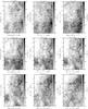 |
Fig. 9 HI channel maps in the area of the Monoceros SNR for the velocity range from +4 km s-1 to +25 km s-1, averaged over 11 consecutive channels, yielding a velocity resolution of ~2 km s-1. The central LSR velocities are indicated above each panel. Total intensities of 6 cm continuum emission smoothed to 10′ are overlaid as contours. |
4.3. Strength of the magnetic field in the western shell
We can estimate the magnetic field strength in the western shell by assuming energy
equipartition between the magnetic field and electrons and protons in the SNR shell. We
implemented the revised equipartition formula by Beck
& Krause (2005), which uses the number density ratio K
instead of the total energies of cosmic ray protons and electrons in classical
equipartition estimates. Assuming the synchrotron emission is concentrated in the SNR
filamentary shell, the radio emissivity
Lν/V
averaged over the source’s volume is replaced by the surface brightness over the
line-of-sight path length through the emitting
region Iν/l.
Therefore, 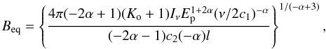 (1)where,
Iν is the synchrotron intensity at
frequency ν and α the synchrotron spectral index of
−0.4. Ko is a constant ratio of number densities of protons
and electrons in the energy range, which is assumed to be 1.
Ep is the proton rest energy. c1
and c2 are constants (see the Appendix of Beck & Krause 2005). We integrated the flux
density at 6 cm for the western shell section centered
at
(1)where,
Iν is the synchrotron intensity at
frequency ν and α the synchrotron spectral index of
−0.4. Ko is a constant ratio of number densities of protons
and electrons in the energy range, which is assumed to be 1.
Ep is the proton rest energy. c1
and c2 are constants (see the Appendix of Beck & Krause 2005). We integrated the flux
density at 6 cm for the western shell section centered
at  ((
(( ), and obtained a value of
11 Jy. The radio intensity of the western shell is
about Iν = 0.2 × 10⁻¹⁸ erg s-1 cm-2 Hz-1 sr-1.
We estimate the thickness of the western filament from high angular resolution 11 cm data
to be ~13′, about 10% of the radius of the SNR. The thickness of the filament is about
6 pc, and the total path through the interacting zone is l ~ 49 pc at a
distance of 1.6 kpc. The estimated equipartition magnetic field
Beq is about 9.5 μG, corresponding to a
factor of ~3−4 enhancement of the mean ISM field of
Btot 2−3 μG (Han et al. 2006).
), and obtained a value of
11 Jy. The radio intensity of the western shell is
about Iν = 0.2 × 10⁻¹⁸ erg s-1 cm-2 Hz-1 sr-1.
We estimate the thickness of the western filament from high angular resolution 11 cm data
to be ~13′, about 10% of the radius of the SNR. The thickness of the filament is about
6 pc, and the total path through the interacting zone is l ~ 49 pc at a
distance of 1.6 kpc. The estimated equipartition magnetic field
Beq is about 9.5 μG, corresponding to a
factor of ~3−4 enhancement of the mean ISM field of
Btot 2−3 μG (Han et al. 2006).
5. Neutral hydrogen morphology
5.1. HI associated with the Monoceros SNR
The GALFA-HI survey covers a velocity range from −700 km s-1 to +700 km s-1 (all HI velocities are with respect to the local standard of rest (LSR)), with a velocity resolution of 0.18 km s-1. Raimond (1966) and Riddle (1972) have shown that a neutral hydrogen shell with an HI cavity inside is located outside of the Monoceros optical filament. The GALFA-HI image has much better resolution and sensitivity and reveals many detailed structures.
The 0.8−1.6 kpc distance corresponds to a velocity range of +8−15 km s-1, according to the Galactic rotation model (Fich et al. 1989: R0 = 8.5 kpc and Θ0 = 220 km s-1). We inspected the entire data cube of this complex region from the GALFA-HI survey in the velocity range between 0 km s-1 and +30 km s-1, looking for structures morphologically related to the SNR.
Figure 9 displays the HI channel maps after averaging over 11 consecutive channels (~2 km s-1) within the velocity interval from +4 to +25 km s-1. The central velocity of each image is indicated at the top. Contours of 6 cm total intensity (smoothed to 10′) are overlaid to indicate the Monoceros complex region. Toward this region, neutral hydrogen filamentary structures caused by stellar winds from the OB associations of Mon OB1 and Mon OB2 are visible across the entire region. The large-scale distribution of neutral hydrogen gas shows a density gradient toward the Rosette molecular complex (RMC). The HI shell related to the RMC lies between +5 km s-1 and +25 km s-1, with a lower emission toward the southern shell of the Monoceros SNR, which is consistent with the result in Kuchar & Bania (1993).
We have identified a partial neutral hydrogen shell surrounding the western SNR, which we
believe is associated with the SNR. This shell structure is distributed over velocities
between +7 km s-1 and +22 km s-1 with a thickness of ~13′. It
lies slightly outside the spherical outline of the remnant, in particular, in the
southwestern direction using Galactic coordinates, and seems to have expanded ahead of the
radio shell. This is similar to the case of another likely old SNR, the North Polar Spur
(Loop I) (Berkhuijsen et al. 1970). However, the HI
shell is well associated with the 60 μm emission (Fig. 3), suggesting that this shell could have been blown out
by strong stellar winds from the progenitor of the SNR before the explosion. The 21 cm
line emission is weak in the eastern SNR sector. It seems that the SNR blast wave has
expanded into a medium of lower density in this direction. In the southern SNR region, the
HI shell features are mixed with those of the Rosette Nebula. However, a small section of
possible shell structure is seen in the HI emission for the velocity range +10 to
14 km s-1, projecting from the east of the Rosette Nebula. This is prominent,
being 0 5 long with a
thickness of 10′ in the +12 km s-1 channel map, and is well associated with the
new shell-like radio continuum feature in the southern shell.
5 long with a
thickness of 10′ in the +12 km s-1 channel map, and is well associated with the
new shell-like radio continuum feature in the southern shell.
In Fig. 10 we present the result for the integrated HI column densities over the velocity range +4 to +25 km s-1. Weak HI emission segments associated with the eastern radio shell of the Monoceros SNR emerge after the large-scale diffuse emission has been subtracted using the “unsharp-masking” procedure described by Sofue & Reich (1979). A cavity with an angular diameter of about 3.8° is visible, coinciding with the Monoceros SNR.
Assuming the HI emission to be optically thin, we calculate the average column density for the northwestern shell to be about 5.5 × 1020 cm-2. If a physical association exists, with a distance of 1.6 kpc, the thickness of the half-shell of 13′ with a 1.9° radius corresponds to a swept-up mass (mHN(HI)) of about 4140 M⊙, assuming the southern shell has a similar column density to the western shell. The average density in the HI-shell is then about n ~ (N/L) = 3.6 cm-3, with a line-of-sight depth within the shell of 49 pc. If this mass of neutral gas had originally been uniformly distributed within a sphere of radius 1.9°, the pre-explosion ambient density would have been 0.27 cm-3, consistent with the ambient density of 0.34 cm-3 estimated by Odegard (1986), according to the Chevalier formula (Chevalier 1974). The evacuation by the action of stellar winds within the Mon OB2 association and the progenitor may cause the low-density environment.
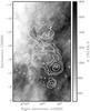 |
Fig. 10 Integrated HI intensities for the velocity range from +4 km s-1 to +25 km s-1 with contours of 6 cm continuum emission overlaid, having levels of 10, 30, 120, and 640 mK. |
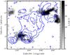 |
Fig. 11 Integrated CO-intensities for the velocity range from 0 km s-1 to +30 km s-1 with 6 cm continuum contours overlaid, having levels of 10, 30, 120, and 640 mK. |
5.2. CO associated with the Monoceros SNR
We inspected the CO images of this region obtained by Oliver et al. (1996). There are weak CO clouds in the direction of the enhanced radio continuum emission of the western shell, with velocities ranging from −3.1 km s-1 to +9.4 km s-1, and enhanced CO emission is found toward the southern shell, with velocities ranging from +10 to +30 km s-1. The Cone cloud adjacent to the northwest of the Monoceros SNR has an average velocity of +7 km s-1. This cloud is the progenitor of the young open cluster NGC 2264 and belongs to the Mon OB1 association (Oliver et al. 1996).
In Fig. 11, we show the integrated 12CO emission from Oliver et al. (1996) in the velocity interval 0 < v < +30 km s-1 with contours of the 6 cm continuum emission overlaid. The molecular cloud associated with the RMC has a ring shape around the nebula with a gap toward the Monoceros SNR. Based on the associated CO morphology and the fact that the Monoceros SNR has a similar velocity to that of the RMC, we suggest that the Monoceros SNR is interacting with the RMC and that the progenitor of the Monoceros SNR comes from the RMC.
5.3. Interaction with the Rosette Nebula
The high-resolution HI channel maps provide evidence that the Monoceros SNR is interacting with the Rosette Nebula. In the integrated HI emission map of Fig. 10, the Rosette Nebula appears to have broken into the Monoceros SNR area outlined by its outer HI shell. HI shell associated with the Rosette Nebula presents a ring shape with a minimum in the direction of the Monoceros SNR. In the channel maps of Fig. 9, a small section of possible HI shell structure is seen at v ~ +12 km s-1 projecting from the east of the Rosette Nebula, coinciding closely with the possible new radio shell. This feature might have a relationship with the interaction between the Monoceros SNR and the Rosette Nebula, and is possibly caused by the shock of the SNR or stellar winds in the Rosette Nebula.
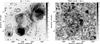 |
Fig. 12 Upper panel: Hα emission overlaid with 11 cm continuum contours having the same levels as for Fig. 1. Lower panel: ROSAT X-ray emission smoothed to 10′ angular resolution overlaid with 6 cm total intensity contours that have the same levels as for Fig. 2. |
It has been previously speculated that the formation of the cluster NGC 2244 was triggered by an encounter between the Monoceros SNR and the RMC (Townsley et al. 2003). Morphologically, it seems that the progenitor of the SNR exploded first and its shock formed a well-shaped shell. Ionized by the cluster NGC 2244 the expansion of the Rosette Nebula kept growing in size into the SNR shell. However, the SNR’s age has been estimated to be 0.3−5 × 10⁵ yr (Welsh et al. 2001). The main-sequence turnoff age of the cluster is about 1.9 Myr (Park & Sung 2002), which suggests that the cluster formed earlier than any possible encounter with the SNR. The kinetic energy of the expansion of the Rosette Nebula was about ~3.8 × 1048 erg (Kuchar & Bania 1993), which is smaller than the typical SNR explosion energy of 1051 erg. Although there is little nonthermal radio emission detected in the Rosette Nebula, it is still possible that the shock of the Monoceros SNR has broken into the Rosette Nebula at some places, possibly the new radio shell region, and is triggering new star formation in the cluster.
Despite the fact that no detection of maser emission has been reported in the radio survey at 1720.5 MHz by Frail et al. (1996), the Monoceros SNR has been interpreted as interacting with the atomic and molecular components of the RMC, based on enhanced line widths of H109α and Hα emission (Fountain et al. 1979) and similar velocity of Hα emission in the contact region (Reynolds 1983). EGRET and HESS have detected high-energy γ-ray emission from the overlap region between the Monoceros SNR and the Rosette Nebula, interpreted in terms of π0 decay resulting from collisions between SNR-accelerated particles and the molecular cloud (Jaffe et al. 1997; Torres et al. 2003). For the first time, the present HI observations provide direct morphological evidence of their interaction. The Monoceros SNR has swept up an HI mass of about 4000 M⊙, with a possible break in the shell at +12 km s-1 toward the Rosette Nebula. A number of Galactic SNRs in physical contact with molecular clouds have been summarized by Jiang et al. (2010). A similar case is the SNR HB3, which is interacting with the adjacent HII region W3 and the associated star-formation region (Routledge et al. 1991).
6. Comparison with other multi-band images
To discuss the physical properties and the environment of the Monoceros SNR, we compare multi-wavelength observations. The Monoceros SNR shows diffuse Hα emission associated with most of the SNR shell region, with weak Hα emission extending outside the southwest shell (Fig. 12). The diffuse emission in the area east of the SNR represents a low-density environment, which results in a less compressed magnetic field and thus reduced efficiency of particle acceleration. The radio filaments are well correlated with the optical filaments ([NII]) (Davies et al. 1978), except for the inner western filament. This correlation is not seen in the optical image, probably due to lower temperatures/densities in the radio filaments.
The Monoceros IRIS 60 μm dust emission with 6 cm total intensity contours superposed is shown in Fig. 3. The shell-associated dust emission projecting from the eastern spur of the Rosette Nebula is enhanced with high ISM density. The dust emission envelope in the western region is outside the radio shell and is associated with the diffuse optical shell (Davies et al. 1978). It is also well circumscribed by the HI shell, suggesting that the dust there has been ionized by a pre-shock caused by stellar winds from the progenitors.
The Monoceros image (0.56−1.21 keV) from the ROSAT soft X-ray all-sky survey (Snowden et al. 1997) is shown in Fig. 12, contours of 6 cm total intensity overlaid. Diffuse X-ray emission is located on the rim of the remnant and coincides with the densest region of optical filaments, as expected for a young SNR in the Sedov phase. In the eastern SNR shell, the X-ray emission is located outside the boundary of the radio contours, which are assumed to trace the outer SNR shock, indicating more diffuse emission in the weak eastern shell.
Leahy et al. (1985, 1986) fitted the weak X-ray emission detected by the Einstein X-ray satellite concluding that the initial density of the medium in which the Monoceros supernova occurred was 0.003 cm-3, and that the expansion of the SNR proceeds in a non-homogeneous multi-component medium. The HI environment confirms this and shows a gradient of density. The Monoceros SNR probably expanded in a pre-existing cavity generated by the progenitor. In this case, the cavity would have had to be extremely large, about 105 pc, which may have required more than one star to make. The shock recently encountered the interstellar material, which turned it into a bright emitter at radio wavelengths.
7. Summary
After subtraction of the inner thermal emission and compact extragalactic sources, we obtained integrated flux densities of 120.8 ± 9.9 Jy at 21 cm, 89.7 ± 7.9 Jy at 11 cm, and 73.4 ± 3.5 Jy at 6 cm for the Monoceros SNR. The spectral index from these three wavelengths is about α = −0.41 ± 0.16, which was confirmed by TT-plots. A new southern shell branch was found that likely belongs to the Monoceros SNR, based on its spectral index of ~−0.5. The distribution of spectral index over the SNR shows some variations and steepens toward the western inner filamentary region, corresponding to a weaker shock compression.
Strong polarized emission was observed from the western filament of the Monoceros SNR at 6 cm and 21 cm, indicating the presence of a strong regular magnetic field component. The RM values there are ambiguous and are typically 30 ± 77n rad m-2, with n = 1 being the favored value. The magnetic field in the western shell region is estimated to be 9.5 μG.
The case for interaction between the Monoceros SNR and the Rosette Nebula is strengthened by the HI data. We identify partial neutral hydrogen shell structures at LSR velocities of +15 km s-1 circumscribing the continuum emission. The HI shell has swept up a mass of about 4000 M⊙ for a distance of 1.6 kpc. The Monoceros SNR has probably triggered part of the star formation in the Rosette Nebula. The western HI shell is found to be well correlated with the dust emission outside of the radio shell, indicating that the Monoceros SNR is evolving within a cavity blown-out by the progenitor and that the SNR is still in the Sedov phase.
Acknowledgments
The 6 cm data were obtained with a receiver system from the MPIfR mounted at the Nanshan 25 m telescope at the Urumqi Observatory of NAOC. We thank the helpful Urumqi staff and people in the Sino-German 6 cm survey team for their contribution to the hard work. The GALFA-HI survey was obtained with a 7-beam feed array at the Arecibo Observatory. We are grateful to the staff at the Arecibo Observatory and the GALFA-HI survey team for conducting the GALFA-HI observations. This research was supported by the National Science Foundation of China (grant 11073028). M.Z. acknowledges support from the “Hundred-talent program” of the Chinese Academy of Sciences. We thank Dr. Youling Yue and Dr. Lei Qian for useful discussions and helpful instruction during this work. We thank the anonymous referee for his instructive and useful comments. We also thank Dr. James Wicker for proofreading the manuscript.
References
- Beck, R., & Krause, M. 2005, Astron. Nachr., 326, 414 [NASA ADS] [CrossRef] [Google Scholar]
- Bell, A. R. 1978a, MNRAS, 182, 147 [NASA ADS] [CrossRef] [Google Scholar]
- Bell, A. R. 1978b, MNRAS, 182, 443 [NASA ADS] [CrossRef] [Google Scholar]
- Berkhuijsen, E. M., Haslam, C. G. T., & Salter, C. J. 1970, Nature, 225, 364 [NASA ADS] [CrossRef] [Google Scholar]
- Broadbent, A., Osborne, J. L., & Haslam, C. G. T. 1989, MNRAS, 237, 381 [NASA ADS] [CrossRef] [Google Scholar]
- Chevalier, R. A. 1974, ApJ, 188, 501 [NASA ADS] [CrossRef] [Google Scholar]
- Cusumano, G., Maccarone, M. C., Nicastro, L., Sacco, B., & Kaaret, P. 2000, ApJ, 528, 25 [Google Scholar]
- Davies, R. D. 1963, The Observatory, 83, 172 [NASA ADS] [Google Scholar]
- Davies, R. D., Elliott, K. H., Goudis, C., Meaburn, J., & Tebbutt, N. J. 1978, A&AS, 31, 271 [NASA ADS] [Google Scholar]
- Day, G. A., Caswell, J. L., & Cooke, D. J. 1972, Aust. J. Phys. Astrophys. Suppl., 25, 1 [NASA ADS] [Google Scholar]
- Dickel, J. R., & Denoyer, L. K. 1975, AJ, 80, 437 [NASA ADS] [CrossRef] [Google Scholar]
- Fiasson, A., Hinton, J. A., Gallant, Y., et al. 2008, in International Cosmic Ray Conference, 2, 719 [Google Scholar]
- Fich, M., Blitz, L., & Stark, A. A. 1989, ApJ, 342, 272 [NASA ADS] [CrossRef] [Google Scholar]
- Fountain, W. F., Gary, G. A., & Odell, C. R. 1979, ApJ, 229, 971 [NASA ADS] [CrossRef] [Google Scholar]
- Frail, D. A., Goss, W. M., Reynoso, E. M., et al. 1996, AJ, 111, 1651 [NASA ADS] [CrossRef] [Google Scholar]
- Fürst, E., & Reich, W. 2004, in The Magnetized Interstellar Medium, eds. B. Uyaniker, W. Reich, & R. Wielebinski, 141 [Google Scholar]
- Fürst, E., Reich, W., & Sofue, Y. 1987, A&AS, 71, 63 [NASA ADS] [CrossRef] [MathSciNet] [PubMed] [Google Scholar]
- Fürst, E., Reich, W., Reich, P., & Reif, K. 1990, A&AS, 85, 691 [NASA ADS] [Google Scholar]
- Gao, X. Y., Reich, W., Han, J. L., et al. 2010, A&A, 515, A64 [NASA ADS] [CrossRef] [EDP Sciences] [Google Scholar]
- Gao, X. Y., Han, J. L., Reich, W., et al. 2011, A&A, 529, A159 [NASA ADS] [CrossRef] [EDP Sciences] [Google Scholar]
- Graham, D. A., Haslam, C. G. T., Salter, C. J., & Wilson, W. E. 1982, A&A, 109, 145 [NASA ADS] [Google Scholar]
- Han, J. L., Manchester, R. N., Lyne, A. G., Qiao, G. J., & van Straten, W. 2006, ApJ, 642, 868 [NASA ADS] [CrossRef] [Google Scholar]
- Holden, D. J. 1968, MNRAS, 141, 57 [NASA ADS] [Google Scholar]
- Jaffe, T. R., Bhattacharya, D., Dixon, D. D., & Zych, A. D. 1997, ApJ, 484, 129 [Google Scholar]
- Jiang, B., Chen, Y., Wang, J., et al. 2010, ApJ, 712, 1147 [NASA ADS] [CrossRef] [Google Scholar]
- Kaaret, P., Piraino, S., Halpern, J., & Eracleous, M. 1999, ApJ, 523, 197 [NASA ADS] [CrossRef] [Google Scholar]
- Kuchar, T. A., & Bania, T. M. 1993, ApJ, 414, 664 [NASA ADS] [CrossRef] [Google Scholar]
- Leahy, D. A., Naranan, S., & Singh, K. P. 1985, MNRAS, 213, 15 [NASA ADS] [Google Scholar]
- Leahy, D. A., Naranan, S., & Singh, K. P. 1986, MNRAS, 220, 501 [NASA ADS] [CrossRef] [Google Scholar]
- Milne, D. K., & Dickel, J. R. 1974, Aust. J. Phys., 27, 549 [Google Scholar]
- Milne, D. K., & Hill, E. R. 1969, Aust. J. Phys., 22, 211 [NASA ADS] [CrossRef] [Google Scholar]
- Miville-Deschênes, M.-A., & Lagache, G. 2005, ApJS, 157, 302 [NASA ADS] [CrossRef] [Google Scholar]
- Odegard, N. 1986, ApJ, 301, 813 [NASA ADS] [CrossRef] [Google Scholar]
- Oliver, R. J., Masheder, M. R. W., & Thaddeus, P. 1996, A&A, 315, 578 [NASA ADS] [Google Scholar]
- Park, B.-G., & Sung, H. 2002, AJ, 123, 892 [NASA ADS] [CrossRef] [Google Scholar]
- Peek, J. E. G., Heiles, C., Douglas, K. A., et al. 2011, ApJS, 194, 20 [NASA ADS] [CrossRef] [Google Scholar]
- Raimond, E. 1966, Bull. Astron. Inst. Netherlands, 18, 191 [NASA ADS] [Google Scholar]
- Reich, W. 2006, in Cosmic Polarization 2006, ed. R. Fabbri, Research Signpost, 91 [arXiv:astro-ph/0603465] [Google Scholar]
- Reich, W., Reich, P., & Fuerst, E. 1990, A&AS, 83, 539 [NASA ADS] [Google Scholar]
- Reynolds, R. J. 1983, ApJ, 268, 698 [NASA ADS] [CrossRef] [Google Scholar]
- Riddle, R. K. 1972, Ph.D. Thesis, University of Maryland, College Park [Google Scholar]
- Routledge, D., Dewdney, P. E., Landecker, T. L., & Vaneldik, J. F. 1991, A&A, 247, 529 [NASA ADS] [Google Scholar]
- Snowden, S. L., Egger, R., Freyberg, M. J., et al. 1997, ApJ, 485, 125 [NASA ADS] [CrossRef] [Google Scholar]
- Sofue, Y., & Reich, W. 1979, A&AS, 38, 251 [NASA ADS] [Google Scholar]
- Taylor, A. R., Stil, J. M., & Sunstrum, C. 2009, ApJ, 702, 1230 [NASA ADS] [CrossRef] [Google Scholar]
- Torres, D. F., Romero, G. E., Dame, T. M., Combi, J. A., & Butt, Y. M. 2003, Phys. Rep., 382, 303 [NASA ADS] [CrossRef] [Google Scholar]
- Townsley, L. K., Feigelson, E. D., Montmerle, T., et al. 2003, ApJ, 593, 874 [NASA ADS] [CrossRef] [Google Scholar]
- Turtle, A. J., Pugh, J. F., Kenderdine, S., & Pauliny-Toth, I. I. K. 1962, MNRAS, 124, 297 [NASA ADS] [CrossRef] [Google Scholar]
- Velusamy, T., & Kundu, M. R. 1974, A&A, 32, 375 [NASA ADS] [Google Scholar]
- Welsh, B. Y., Sfeir, D. M., Sallmen, S., & Lallement, R. 2001, A&A, 372, 516 [NASA ADS] [CrossRef] [EDP Sciences] [Google Scholar]
- Wolleben, M., Landecker, T. L., Reich, W., & Wielebinski, R. 2006, A&A, 448, 411 [NASA ADS] [CrossRef] [EDP Sciences] [Google Scholar]
All Figures
|
Fig. 1 Effelsberg 21 cm and 11 cm continuum images of the Monoceros SNR, with angular resolutions of 9.4′ and 4.4′ respectively. Contours at 21 cm start from 100 mK TB and increase by 2n × 80 mK TB (n = 0,1,2,3,...). Contours at 11 cm are drawn according to 2n × 30 mK TB, with n = 0,1,2,3,... |
| In the text | |
|
Fig. 2 Urumqi 6 cm total intensity map of the Monoceros SNR at an angular resolution of 9.5′. Polarization vectors in the B-field direction (E+90°) are overlaid. The length of the bars is proportional to PI, with a polarized intensity of 1 mK TB, corresponding to a bar-length of 2′. Total intensity contours are drawn according to 2n × 10 mK TB, with n = 0,1,2,3,... |
| In the text | |
|
Fig. 3 IRIS 60 μm emission of the same area as in the preceding radio continuum images. Resolution is 2′. Contours of 6 cm total intensity are overlaid and have the same levels as for Fig. 2. |
| In the text | |
|
Fig. 4 Plot of the brightness temperature TB,21 against the brightness I60. The best-fit straight line corresponds to a slope of 23.6 mK MJy-1 sr. |
| In the text | |
|
Fig. 5 Spectral index from integrated flux densities of the Monoceros SNR. |
| In the text | |
|
Fig. 6 TT-plots between Urumqi 6 cm data and the Effelsberg 21 cm data (as examples) for the eastern shell, northwest filamentary shell, and newly identified southern branch shell of the Monoceros SNR. |
| In the text | |
|
Fig. 7 Temperature spectral index map of the Monoceros SNR from 21/11/6 cm maps. Regions where the random error exceeds 0.06 have been blanked out. Contours of 6 cm total intensity with the same levels as Fig. 2 are overlaid. |
| In the text | |
|
Fig. 8 DRAO 21 cm polarized intensity map of the Monoceros SNR at an angular resolution of 36′. Polarization vectors in the B-field direction (E+90°) are overlaid. The length of the vectors is proportional to PI. A polarized intensity of 1 mK TB corresponds to a length of 0.05′. Contours show total intensities starting at 200 mK TB and increasing by 2n × 60 mK TB (n = 0,1,2,3,...). The positions of RM sources in Taylor et al. (2009) are indicated by crosses, with lengths proportional to the RM values. |
| In the text | |
|
Fig. 9 HI channel maps in the area of the Monoceros SNR for the velocity range from +4 km s-1 to +25 km s-1, averaged over 11 consecutive channels, yielding a velocity resolution of ~2 km s-1. The central LSR velocities are indicated above each panel. Total intensities of 6 cm continuum emission smoothed to 10′ are overlaid as contours. |
| In the text | |
|
Fig. 10 Integrated HI intensities for the velocity range from +4 km s-1 to +25 km s-1 with contours of 6 cm continuum emission overlaid, having levels of 10, 30, 120, and 640 mK. |
| In the text | |
|
Fig. 11 Integrated CO-intensities for the velocity range from 0 km s-1 to +30 km s-1 with 6 cm continuum contours overlaid, having levels of 10, 30, 120, and 640 mK. |
| In the text | |
|
Fig. 12 Upper panel: Hα emission overlaid with 11 cm continuum contours having the same levels as for Fig. 1. Lower panel: ROSAT X-ray emission smoothed to 10′ angular resolution overlaid with 6 cm total intensity contours that have the same levels as for Fig. 2. |
| In the text | |
Current usage metrics show cumulative count of Article Views (full-text article views including HTML views, PDF and ePub downloads, according to the available data) and Abstracts Views on Vision4Press platform.
Data correspond to usage on the plateform after 2015. The current usage metrics is available 48-96 hours after online publication and is updated daily on week days.
Initial download of the metrics may take a while.