| Issue |
A&A
Volume 544, August 2012
|
|
|---|---|---|
| Article Number | A143 | |
| Number of page(s) | 6 | |
| Section | The Sun | |
| DOI | https://doi.org/10.1051/0004-6361/201219763 | |
| Published online | 15 August 2012 | |
Cut-off wavenumber of Alfvén waves in partially ionized plasmas of the solar atmosphere
1 Space Research Institute, Austrian Academy of Sciences, Schmiedlstrasse 6, 8042 Graz, Austria
e-mail: This email address is being protected from spambots. You need JavaScript enabled to view it.
; This email address is being protected from spambots. You need JavaScript enabled to view it.
2 Departament de Matemàtiques i Informàtica. Universitat de les Illes Balears, 07122 Palma de Mallorca, Spain
e-mail: This email address is being protected from spambots. You need JavaScript enabled to view it.
3 Departament de Física, Universitat de les Illes Balears, 07122 Palma de Mallorca, Spain
e-mail: This email address is being protected from spambots. You need JavaScript enabled to view it.
4 Abastumani Astrophysical Observatory at Ilia State University, University St. 2, Tbilisi, Georgia
Received: 6 June 2012
Accepted: 17 July 2012
Abstract
Context. Alfvén wave dynamics in partially ionized plasmas of the solar atmosphere shows that there is indeed a cut-off wavenumber, i.e. the Alfvén waves with wavenumbers higher than the cut-off value are evanescent. The cut-off wavenumber appears in single-fluid magnetohydrodynamic (MHD) approximation but it is absent in a multi-fluid approach. Up to now, an explanation for the existence of the cut-off wavenumber is still missing.
Aims. The aim of this paper is to point out the reason for the appearance of a cut-off wavenumber in single-fluid MHD.
Methods. Beginning with three-fluid equations (with electrons, protons and neutral hydrogen atoms), we performed consecutive approximations until we obtained the usual single-fluid description. We solved the dispersion relation of linear Alfvén waves at each step and sought the approximation responsible of the cut-off wavenumber appearance.
Results. We have found that neglecting inertial terms significantly reduces the real part of the Alfvén frequency although it never becomes zero. Therefore, the cut-off wavenumber does not exist at this stage. However, when the inertial terms together with the Hall term in the induction equation are neglected, the real part of the Alfvén frequency becomes zero.
Conclusions. The appearance of a cut-off wavenumber, when Alfvén waves in partially ionized regions of the solar atmosphere are studied, is the result of neglecting inertial and Hall terms, therefore it has no physical origin.
Key words: Sun: atmosphere / Sun: oscillations
© ESO, 2012
1. Introduction
Cut-off wavenumbers in fully ionized resistive magnetohydrodynamic (MHD) have been reported in several classical textbooks. For instance, in the chapter on the thermal instability of a layer of fluid heated from below when a magnetic field is present, Chandrasekhar (1961) described the behavior of Alfvén waves in a viscous and resistive medium. In this case, the Alfvén wave frequency, ω, is given by 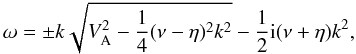 (1)where VA is the Alfvén speed, ν the kinematic viscosity, η the magnetic diffusivity, and k the wavenumber. This expression clearly points out that for a value of the wavenumber such as
  (2)the real part of the frequency becomes zero, and only the imaginary part of the frequency remains. The cut-off wavenumber means that waves with a wavenumber higher than the cut-off value are evanescent. Therefore, Eq. (2) provides us with the cut-off wavenumber for resistive and viscous plasmas when the single-fluid approximation is used. When viscosity is negligible, but resistivity still exists (resistive plasma), this cut-off wavenumber is modified by keeping only the resistivity in the denominator of Eq. (2). Chandrasekhar (1961) made no explicit comment about this cut-off wavenumber, only pointed out that when viscosity or resistivity are present, Alfvén waves are damped. Ferraro & Plumpton (1961) and Kendall & Plumpton (1964) considered the effects of finite conductivity on hydromagnetic waves, and showed that for ηk < 2VA, we have time-damped waves, while for ηk > 2VA there is no wave propagation at all. Furthermore, Cramer (2001) has pointed out the same effect, showing that when the wavenumber becomes greater than 2Rm/L, where Rm is the magnetic Reynolds number and L a reference length, the real part of the Alfvén wave frequency becomes zero. Although some of the above reported textbooks have shown that there is a cut-off wavenumber, none of them has investigated the reason for its presence in resistive single-fluid MHD and its physical meaning, if any.
On the other hand, the real part of Eq. (1) can be written as  (3)with
  (4)representing a modified Alfvén speed that goes to zero for the cut-off wavenumber, i.e. the wave ceases its propagation.
Significant parts of the solar atmosphere, namely photosphere, chromosphere and prominences, are only partially ionized. Collisions between different plasma species generally lead to the damping of waves in magnetized plasmas. Neutral atoms may enhance the damping of transverse waves through ion-neutral collision (Braginskii 1965; Khodachenko et al. 2004; Carbonell et al. 2010; Zaqarashvili et al. 2011a,b) and may lead to heating of the ambient plasma (Khomenko and Collados 2012). In partially ionized plasmas and in an astrophysical context, Kulsrud & Pearce (1969) studied the interaction between cosmic rays and Alfvén waves in the interstellar medium, and showed that a cut-off wavenumber appeared there as well. Balsara (1996) studied MHD wave propagation in molecular clouds in the single-fluid approximation, reporting that Alfvén and fast waves become completely damped when the wavenumber attains a certain value. Recently, and in the context of solar prominence oscillations, cut-off wavenumbers have been reported again. Forteza et al. (2007, 2008), Barceló et al. (2011) and Soler et al. (2011) used the single-fluid approximation to study the damping of MHD waves produced by ion-neutral collisions in an unbounded medium with prominence physical properties. These authors found that the cut-off wavenumber for Alfvén waves is given by  (5)with θ the propagation angle with respect to the magnetic field, and ηc the Cowling diffusivity. In this case, the modified Alfvén speed (Barceló et al. 2011) is given by
 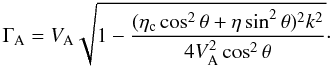 (6)For fully ionized resistive plasmas, η = ηc and, for parallel propagation, we recover the Kendall & Plumpton (1964) cut-off wavenumber. When fast and slow waves are coupled, the numerical value of the cut-off wavenumber for fast waves is similar to that of Alfvén waves, but for parallel propagation fast waves decouple, becoming Alfvén waves, and their cut-off wavenumber is exactly the same as for Alfvén waves. Singh & Krishnan (2010) studied the behavior of Alfvén waves in the partially ionized solar atmosphere and they also reported the cut-off wavenumber.
Since time-damped transversal oscillations have been observed in the fine structure of solar filaments, Soler et al. (2009a,b) modeled this fine structure as magnetic cylinders filled with partially ionized plasma, which has prominence physical properties, and studied the time damping of transverse oscillations produced by ion-neutral collisions and resonant absorption. Again, cut-off wavenumbers for fast and Alfvén waves appear, as described by Eq.(5).
The behaviour of the cut-off wavenumber in a partially ionised plasma can be understood by writing its expression in terms of η and ηC. The Cowling magnetic diffusivity, ηC, is ![Mathematical equation: \begin{eqnarray} \eta_{\rm C} = \frac{1}{4 \pi}\left[\frac{m_{\rm e} c^2}{n_{\rm e} e^2}\left (\frac{1}{\tau_{\rm ei}}+\frac{1}{\tau_{\rm en}}\right )+\frac{\xi_{\rm n}^2 B_0^2}{\alpha_{\rm n}}\right], \end{eqnarray}](/articles/aa/full_html/2012/08/aa19763-12/aa19763-12-eq21.png) (7)where τen and τei are the electron-neutral and electron-ion collisional times, respectively, ξn represents the relative density of neutrals, and αn is a friction coefficient whose expression is
(7)where τen and τei are the electron-neutral and electron-ion collisional times, respectively, ξn represents the relative density of neutrals, and αn is a friction coefficient whose expression is  (8)with Σin the ion-neutral collision cross-section. The Spitzer magnetic diffusivity, η, is
 ![Mathematical equation: \begin{eqnarray} \eta = \frac{c^2}{4 \pi} \frac{m_{\rm e} }{n_{\rm e} e^2}\left [\frac{1}{\tau_{\rm ei}}+\frac{1}{\tau_{\rm en}}\right ], \end{eqnarray}](/articles/aa/full_html/2012/08/aa19763-12/aa19763-12-eq28.png) (9)then, the cut-off wavenumber, k, given by Eq. (5), becomes
(9)then, the cut-off wavenumber, k, given by Eq. (5), becomes ![Mathematical equation: \begin{equation} k= \frac{2 V_{\rm A} \cos \theta}{\frac{1}{4 \pi} \Big[\frac{m_{\rm e} c^2}{n_{\rm e} e^2}\Big(\frac{1}{\tau_{\rm ei}}+\frac{1}{\tau_{\rm en}}\Big)+\frac{\xi_{\rm n}^2 B_0^2}{\alpha_{\rm n}}\cos^2 \theta \Big] }\cdot \end{equation}](/articles/aa/full_html/2012/08/aa19763-12/aa19763-12-eq29.png) (10)On the other hand, as reported by Cramer (2001), the cut-off wavenumber, k, can be written in terms of the magnetic Reynolds number. In a partially ionized plasma of the solar atmosphere, the Cowling magnetic diffusivity, ηC, is several orders of magnitude greater than Spitzer’s magnetic diffusivity, η, therefore, neglecting η in Eq. (5), we obtain
(10)On the other hand, as reported by Cramer (2001), the cut-off wavenumber, k, can be written in terms of the magnetic Reynolds number. In a partially ionized plasma of the solar atmosphere, the Cowling magnetic diffusivity, ηC, is several orders of magnitude greater than Spitzer’s magnetic diffusivity, η, therefore, neglecting η in Eq. (5), we obtain  (11)In our case, the magnetic Reynolds number, Rm, could be written as Rm = uL/ηC, where u is a characteristic velocity, which we could take as the Alfvén speed, and L is a characteristic scale-length. Then, Rm can be expressed as Rm = VAL/ηC, and using Eq. (11) we obtain
  (12)Summarizing, cut-off wavenumbers appear when the single-fluid approximation is used to study MHD waves in collisional magnetized astrophysical plasmas. In particular, this topic is relevant in connection with MHD waves in regions of the solar atmosphere such as chromosphere and photosphere, or in chromospheric and coronal solar structures such as spicules or prominences. However, and up to now, an explanation for the existence of the cut-off wavenumber is still missing.
Recently, Zaqarashvili et al. (2011a) have shown that the cut-off wavenumber for Alfvén waves is absent in a two-fluid MHD approximation, where one fluid is the ion-electron gas and the other fluid is the gas of neutral hydrogen. Then, it is clear that the cut-off wavenumber appears as a result of an approximation and is not an intrinsic property of waves.
Here we study the dynamics of linear Alfvén waves in the partially ionized plasma of the solar atmosphere and seek for the reason for the appearance of the cut-off wavenumber. We start from the full multi-fluid linear equations and make consecutive approximations until the usual equations for Alfvén waves in single-fluid MHD are recovered. After each approximation, we derive the corresponding dispersion relations which, once solved, allow us to uncover the approximation responsible for the cut-off wavenumber appearance.
2. Main equations
We study partially ionized plasmas made of electrons (e), ions (i) and neutral (hydrogen) atoms (n). We suppose that each sort of species possess Maxwell velocity distribution, therefore they can be described as separate fluids.
We aim to study the dynamics of Alfvén waves, therefore we consider incompressible plasma. We also neglect the viscosity, the heat flux and the heat production due to collisions between particles. Plasma and unperturbed magnetic field are considered to be homogeneous. Then, linearized fluid equations for each species can be split into perpendicular and parallel components of perturbations with regard to the unperturbed magnetic field. We are interested in Alfvén waves, therefore only perpendicular components are considered. Then, the fluid and Maxwell (without displacement current) equations can be written as  where ma and na are the mass and the number density of particles a, B is the unperturbed magnetic field strength, ua ⊥ and b ⊥ are the velocity and magnetic perturbations perpendicular to the unperturbed magnetic field, E ⊥ and j ⊥ are the perpendicular components of electric field and current density, ea = ± 4.8 × 10⁻¹⁰ statcoul is the charge of electrons and protons (note, that ea = 0 for neutral hydrogen) and c = 2.9979 × 1010 cm s-1 is the speed of light. Plasma is supposed to be quasi-neutral, which means ne = ni. Ra ⊥ is the change of impulse of particles a due to collisions with other sort of particles, which in the case of Maxwell distribution in each sort of particles has the form (Braginskii 1965)
  (17)where αab = αba are coefficients of friction between particles a and b.
For time scales longer than ion-electron and ion-ion collision times, the electron and ion gases can be considered as a single fluid. This significantly simplifies the equations taking into account the smallness of electron mass with regard to the masses of ion and neutral atoms. Then the three-fluid description can be changed by a two-fluid description, where one component is the charged fluid (electron+protons) and the other component is the gas of neutral hydrogen (Zaqarashvili et al. 2011a).
Then we may go a step further and derive the single-fluid MHD equations. We use the total velocity (i.e. velocity of center of mass)  (18)the relative velocity
  (19)and the total density
  (20)where ρa = mana is the density of the corresponding fluid. Then, Eqs. (13)–(16) are rewritten as
 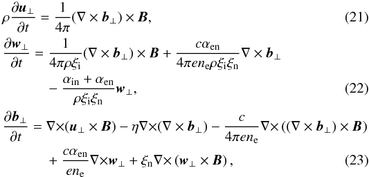 where ξi = ρi/ρ, ξn = ρn/ρ and
 ![Mathematical equation: \begin{equation} \label{etaT} \eta={{c^2}\over {4\pi \sigma}}={{c^2}\over {4\pi e^2 n^2_{\rm e}}}\left [\alpha_{\rm ei}+{{\alpha_{\rm ei}\alpha_{\rm en}}\over {\alpha_{\rm ei}+\alpha_{\rm en}}} \right ]\cdot \end{equation}](/articles/aa/full_html/2012/08/aa19763-12/aa19763-12-eq66.png) (24)The single-fluid Hall MHD equations are obtained from Eqs. (21)–(23) as follows. The inertial term (the left-hand side term in Eq. (22)) is neglected, which is a good approximation for time scales longer than ion-neutral collision time, but fails for the shorter time scales (Zaqarashvili et al. 2011a). Then w ⊥ defined from Eq. (22) is substituted into Eq. (23) and one can obtain the Hall MHD equations
(24)The single-fluid Hall MHD equations are obtained from Eqs. (21)–(23) as follows. The inertial term (the left-hand side term in Eq. (22)) is neglected, which is a good approximation for time scales longer than ion-neutral collision time, but fails for the shorter time scales (Zaqarashvili et al. 2011a). Then w ⊥ defined from Eq. (22) is substituted into Eq. (23) and one can obtain the Hall MHD equations ![Mathematical equation: \begin{eqnarray} \label{V2} \rho{{\partial \vec u_{\perp}}\over {\partial t}}&=&{1\over {4\pi}}(\nabla \times \vec b_{\perp}) \times \vec B, \\ {{\partial \vec b_{\perp}}\over {\partial t}}&=&\nabla \times(\vec u_{\perp} \times \vec B)-{{c}\over {4\pi en_{\rm e}}} \left[1- {{2\xi_{\rm n}\alpha_{\rm en}}\over {\alpha_{\rm in}+\alpha_{\rm en}}}\right]\nabla \notag\\\label{B2} &&\quad\times\left((\nabla \times \vec b_{\perp})\times \vec B \right )+\eta_{\rm c} \nabla^2 \vec b_{\perp}, \end{eqnarray}](/articles/aa/full_html/2012/08/aa19763-12/aa19763-12-eq68.png) where
where 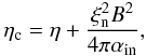 (27)is the Cowling coefficient of magnetic diffusion and the second term in the right side of Eq. (26) is the Hall current term modified by electron-neutral collisions.
 |
Fig. 1 Real part of the dimensionless wave frequency Re(ω) versus the dimensionless Alfvén frequency a = kVA/ωi in partially ionized plasmas, where ωi is the ion gyro-frequency. a) Single-fluid MHD equations with inertial term (dispersion relation given by Eq. (30)); b) single-fluid Hall MHD equations (dispersion relation given by Eq. (31)); c) single-fluid MHD equations without modified Hall current (dispersion relation given by Eq. (35)); d) zoom of the solutions in panels b) (green line) and c) (red line) near x axis. |
The usual single-fluid MHD equations, which are widely used for describing of Alfvén waves in partially ionized plasmas, are obtained from Eqs. (25), (26) after neglecting the modified Hall term in Eq. (26) 
3. Alfvén waves in partially ionized plasmas of the solar atmosphere
We study the propagation of linear Alfvén waves in partially ionized plasmas of the solar atmosphere. Here, and for the numerical calculations, we have chosen physical parameters corresponding to solar quiescent prominences (B = 10 G, ne = 1010 cm-3, T = 8000 K). The unperturbed magnetic field B is directed along the z axis of cartesian frame. Next, we consider the Alfvén wave propagation along the magnetic field, consequently, we perform the Fourier analysis with exp( − iϖt + ikz), where ϖ is the wave frequency and k is the wavenumber.
From Eqs. (21)–(23) the following dispersion relation is obtained ![Mathematical equation: \begin{eqnarray} &&a\delta^2 \nu \left [1+(1+\nu)\zeta \right ]\omega -a \xi_{\rm n} \left [(\pm a + \xi_{\rm i} \omega)\omega -1 \right ]\omega +{\rm i} \delta \Big [a^2 \xi_{\rm n} \omega^2\notag\\ &&+ \nu\Big [\pm a \omega (\zeta-1)-a^2 \zeta \omega^2 +\xi_{\rm i} (1+\zeta(1\mp 2a \omega) \notag\\\label{dispn1} &&+((a^2-1)\zeta-1)\omega^2)\Big ]\Big ]=0, \end{eqnarray}](/articles/aa/full_html/2012/08/aa19763-12/aa19763-12-eq83.png) (30)where ω = ϖ/(kVA), τ = ωe/ωi, a = kVA/ωi, δ = δei/ωe, ν = αin/αei and ζ = αen/αin. Here
(30)where ω = ϖ/(kVA), τ = ωe/ωi, a = kVA/ωi, δ = δei/ωe, ν = αin/αei and ζ = αen/αin. Here  is the Alfvén speed, δei = αei/(mene) is the electron-ion collision frequency, ωi = eB/(cmi) and ωe = eB/(cme) are ion and electron giro-frequencies, respectively.
The dispersion relation given by Eq. (30) has six different solutions. Four of the solutions are Alfvén waves polarized in two perpendicular planes and propagating in opposite directions. The remaining solutions have zero real frequency at low wavenumbers, so they are purely damped oscillations, but they have a low real frequency at high wavenumbers. Here and in the remaining part of the paper we consider only Alfvén waves. The dispersion relation in Eq. (30) has a very involved analytical solution, therefore it has been solved numerically and the solution is plotted in Fig. 1a. This plot shows that there is no cut-off wavenumber and it is similar to the upper plot of Fig. 2 from Zaqarashvili et al. (2011a).
The next approximation is neglecting the inertial term in Eq. (22). This is equivalent to the traditional single-fluid Hall MHD in partially ionized plasmas, and the dispersion relation is given by ![Mathematical equation: \begin{eqnarray} &&\delta^2 \nu^2\xi_{\rm i}^2(1+\zeta)^2\omega^4-2\delta^2 \nu^2 \xi_{\rm i}^2[1+ \zeta(2+\zeta)]\omega^2-\Big [\delta^4 \nu^2 [1 \notag\\ &&+(1+\nu)\zeta]^2+\xi_{\rm n}^4+2\delta^2 \nu (1+\zeta)\xi_{\rm n}^2 +\delta^2 \nu^2 \Big (1+\zeta^2(1-4\xi_{\rm i}) \notag\\ &&+2\xi_{\rm i}^2(1+2\zeta)\Big )\Big ]a^2\omega^2 +\delta^2 \nu^2 (1+\zeta)^2\xi_{\rm i}^2+2{\rm i}a(1+\zeta)\xi_{\rm i} \delta \nu \notag\\\label{dispn21} &&\times\left [ \delta \nu (1+(1+\nu)\zeta)+ \xi_{\rm n}^2 \right ] \omega (\omega^2-1)=0. \end{eqnarray}](/articles/aa/full_html/2012/08/aa19763-12/aa19763-12-eq93.png) (31)The numerical solution of this dispersion relation is shown in Fig. 1b. At low wavenumbers, the wave frequency is Alfvénic, but, when the wavenumber exceeds the value corresponding to the ion-neutral collision frequency (a ≈ 0.00005 on the x axis), the real part of the wave frequency gradually decreases and becomes very small near a ≈ 0.001. Since the real part of the frequency never becomes zero, there is no cut-off wavenumber. Thus, the single-fluid approach in partially ionized plasmas with Hall current term does not include a cut-off wavenumber.
(31)The numerical solution of this dispersion relation is shown in Fig. 1b. At low wavenumbers, the wave frequency is Alfvénic, but, when the wavenumber exceeds the value corresponding to the ion-neutral collision frequency (a ≈ 0.00005 on the x axis), the real part of the wave frequency gradually decreases and becomes very small near a ≈ 0.001. Since the real part of the frequency never becomes zero, there is no cut-off wavenumber. Thus, the single-fluid approach in partially ionized plasmas with Hall current term does not include a cut-off wavenumber.
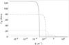 |
Fig. 2 Modified Alfvén speed, ΓA, versus wavenumber for the photosphere (dashed line), the low chromosphere (dotted line), the high chromosphere (dot-dash line), and quiescent prominences (solid line) |
Equation (31) can be significantly simplified as ζ ≪ 1 i.e. αen ≪ αin and it becomes (Pandey & Wardle 2008) ![Mathematical equation: \begin{equation} \label{dispn2} \omega^2+\left [{\rm i}{{\eta_{\rm c} k}\over V_{\rm A}} \pm {{k V_{\rm A}}\over {\omega_{\rm i} \xi_{\rm i}}}\right ] \omega -1=0, \end{equation}](/articles/aa/full_html/2012/08/aa19763-12/aa19763-12-eq99.png) (32)whose analytical solution is given by
(32)whose analytical solution is given by ![Mathematical equation: \begin{equation} \label{frehall} \omega = \frac{1}{2} \left[-\left(\frac{{\rm i} k \eta_{\rm c}}{V_{\rm A}} \pm \frac{k V_{\rm A}}{\xi_{\rm i} \omega_{\rm i}}\right) \pm \sqrt{4+\left(\frac{{\rm i} k \eta_{\rm c}}{V_{\rm A}} \pm \frac{k V_{\rm A}}{\xi_{\rm i} \omega_{\rm i}}\right)^2}\right]\cdot \end{equation}](/articles/aa/full_html/2012/08/aa19763-12/aa19763-12-eq100.png) (33)The real part of the frequency is
(33)The real part of the frequency is 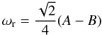 (34)with
  and
and  Equations (33) and (34) clearly show that the wave frequency always has a real part, i.e. the Hall current term (the second term in front of ω in Eq. 32) forbids the appearance of a cut-off wavenumber.
Next, we neglect the modified Hall current term in Eq. (23), which gives the dispersion relation of Alfvén waves commonly used in partially ionized plasmas: 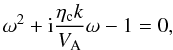 (35)whose analytical solution is
 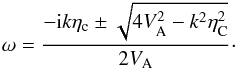 (36)From Eq. (36), and in dimensional form, the real part of the Alfvén frequency can be written as
  (37)where
  (38)represents the modified Alfvén speed for the considered case. From this solution, the modified Alfvén speed becomes zero when
  (39)and it determines the cut-off wavenumber for Alfvén waves. Therefore, Alfvén waves cannot propagate for wavenumbers higher than this cut-off value.
The analytical solution for the real part of the frequency in Eq. (36) is plotted in Fig. 1c and becomes zero near a ≈ 0.001, which corresponds to the analytical cut-off wavenumber defined by Eq. (39). Furthermore, Fig. 1d displays a zoom near the x axis of the solutions corresponding to dispersion relations given by Eqs. (31) and (35), showing that only after removing the modified Hall current term in the induction equation the real part of the wave frequency becomes zero.
The condition of evanescence i.e. (k > kc) can be written as  (40)where
  (41)is the mean ion-neutral collision frequency, and Eq. (40) can be approximated as
  (42)which shows that the Alfvén frequency corresponding to the cut-off wavenumber is lower than the mean ion-neutral collision frequency for weakly ionized plasmas (ξi ≪ ξn), and higher for almost fully ionized plasmas (ξi ≫ ξn).
Hence, the cut-off wavenumber of Alfvén waves in partially ionized plasmas appears after neglecting the inertial term (the left-hand side term in Eq. (22)) and the modified Hall current term in the induction equation (Eq. (26)).
Let us estimate the Alfvén frequency corresponding to the cut-off wavenumber for parameters typical of solar prominence cores (ni = 1010 cm-3, nn = 2 × 1010 cm-3). Then, the cut-off frequency exactly equals the ion-neutral collision frequency δin, which is about 3 s-1. For prominence oscillations, the observed periods are in the range between 30 s (Balthasar et al. 1993) and 10–30 h (Foullon et al. 2009), therefore, since these periods are much longer than the typical collisional timescales, the single-fluid approximation can be safely used when interpreting prominence oscillations in terms of MHD waves.
As we stated in Sect. 1, the above calculations are relevant for MHD waves in different layers and structures of the solar atmosphere. Therefore, from the expression for the modified Alfvén speed (Eq. (38)), the numerical value for the cut-off wavenumber in different partially ionized layers of the solar atmosphere such as the photosphere and the low and high chromosphere, can be obtained. The physical parameters for these regions of the solar atmosphere are taken from the FAL-1993 model (Fontenla et al. 1993), and in Fig. 2 we plot the behavior of the modified Alfvén speed, ΓA versus the wavenumber, k, for the layers mentioned above and for quiescent prominences. This figure shows that in all the considered cases a cut-off wavenumber appears, whose numerical value depends, of course, on the different physical conditions that modify Cowling resistivity. Furthermore, the figure also points out that within a certain range of wavenumbers, the numerical value of the modified Alfvén speed for each region or structure considered coincides (horizontal part of the plots) with the ideal Alfvén speed, VA, as is expected from Eq. (38). Finally, we remark that the single-fluid approximation is valid only for waves whose wavenumbers are lower than the cut-off value.
4. Discussion and conclusion
Consequent approximations from multi-fluid to single fluid MHD allow us to find the stage where the cut-off wavenumber for Alfvén waves appears in partially ionized plasmas of the solar atmosphere. The real part of the wave frequency always exists in full multi-fluid equations, which means that there is no cut-off wavenumber of Alfvén waves. The real part of wave frequency approaches zero, but never vanishes when the inertia of ion-neutral relative velocity are neglected. This approximation corresponds to the single-fluid Hall MHD and hence there is no cut-off wavenumber here, either. On the other hand, the cut-off wavenumber appears when, after neglecting the inertial term, one neglects the modified Hall current term in the induction equation.
The appearance of Alfvén waves is due to the current j⊥, which is perpendicular to b⊥ and k (see Eq. (16)). This current is due to the ion inertia in an oscillating electric field E⊥ and it plays a key role in Alfvén oscillations through the force j⊥ × B (Chen 1988). In the general case, when both electrons and ions move freely into electric and magnetic fields, the collision of plasma particles and neutral atoms may lead only to damping of Alfvén waves and waves with any frequency may propagate in the medium (but remember that the wave frequency should be always lower than ion-electron collision frequency, otherwise the fluid approximation is not valid). When one neglects the electron inertia, i.e. considers the Hall MHD approximation, the electrons are frozen in the magnetic field, but ion inertia is still at play. In this case, the collision between ions and neutrals becomes important for shorter scales and it opposes the current j ⊥ at higher wavenumbers. However, oscillations again exist for all wavelengths due to the Hall current, but the wave frequency is much lower than the Alfvén frequency for shorter wavelengths (see green lines in Fig. 1). The critical point arises when one neglects the Hall current in the induction equation. Then the collision between particles completely blocks the current j ⊥ at higher wavenumbers and leads to the appearances of the cut-off frequency.
Finally, there is still no cut-off wavenumber if one neglects the usual Hall current but retains the electron-neutral collision: the real part of wave frequency very closely approaches the x axis, but never becomes zero. This is because the electrons are not completely frozen into the magnetic field due to the collision with neutrals, and therefore the ion-neutral collision cannot completely block the current j ⊥ at higher wavenumbers.
We note that a cut-off wavenumber may appear for Alfvén waves in the stratified solar atmosphere (Murawski & Musielak 2010, and references therein). But this cut-off wavenumber has a completely different origin because it arises as a result of atmospheric stratification due to the solar gravity.
In summary, the cut-off wavenumber in Alfvén waves in single-fluid partially ionized plasmas is due to the approximations made when proceeding from multifluid to single-fluid equations and is not connected to any physical process. This conclusion is relevant for MHD wave studies in partially ionized regions and structures of the solar atmosphere.
Acknowledgments
The work was supported by the Austrian Fonds zur Förderung der Wissenschaftlichen Forschung (project P21197-N16) and by the European FP7-PEOPLE-2010-IRSES-269299 project- SOLSPANET. J. L. Ballester and M. Carbonell acknowledge the financial support received from MICINN and FEDER Funds under grant AYA2011-22846 and from CAIB through the “Grups Competitius” scheme and FEDER Funds. They also
acknowledge the warm hospitality enjoyed during the visit payed to the Space Research Institute in Graz where this research was started. J. L. Ballester acknowledges the financial support received from the Austrian Academy of Sciences.
References
- Balsara, D. S. 1996, ApJ, 465, 775 [NASA ADS] [CrossRef] [Google Scholar]
- Balthasar, H., Wiehr, E., Schleicher, H., & Wohl, H. 1993, A&A, 277, 635 [NASA ADS] [Google Scholar]
- Barceló, S., Carbonell, M., & Ballester, J. L. 2011, A&A, 525, A60 [NASA ADS] [CrossRef] [EDP Sciences] [Google Scholar]
- Braginskii, S. I. 1965, Rev. Plasma Phys., 1, 205 [NASA ADS] [Google Scholar]
- Carbonell, M., Forteza, P., Oliver, R., & Ballester, J. L. 2010, A&A, 515, A80 [NASA ADS] [CrossRef] [EDP Sciences] [Google Scholar]
- Chandrasekhar, S. 1961, Hydrodynamic and Hydromagnetic Stability (London: Oxford University Press) [Google Scholar]
- Chen, F. F. 1988, Introduction to Plasma Physics and Controlled Fusion (New York: Plenum Press) [Google Scholar]
- Cramer, N. F. 2001, The Physics of Alfvén Waves (Wiley) [Google Scholar]
- Ferraro, V. C. A., & Plumpton, C. 1961, An Introduction to magneto-fluid mechanics (Oxford University Press) [Google Scholar]
- Fontenla, J. M., Avrett, E. H., & Loeser, R. 1993, ApJ, 355, 700 [Google Scholar]
- Forteza, P., Oliver, R., Ballester, J. L., & Khodachenko, M. L. 2007, A&A, 461, 731 [NASA ADS] [CrossRef] [EDP Sciences] [Google Scholar]
- Forteza, P., Oliver, R., & Ballester, J. L. 2008, A&A, 492, 223 [NASA ADS] [CrossRef] [EDP Sciences] [Google Scholar]
- Foullon, C., Verwichte, E., & Nakariakov, V. M. 2009, ApJ, 700, 1658 [NASA ADS] [CrossRef] [Google Scholar]
- Kendall, D. C., & Plumpton, C. 1964, Magnetohydrodynamics with Hydrodynamics (Pergamon Press) [Google Scholar]
- Khodachenko, M. L., Arber, T. D., Rucker, H. O., & Hanslmeier, A. 2004, A&A, 422, 1073 [NASA ADS] [CrossRef] [EDP Sciences] [Google Scholar]
- Khomenko, E., & Collados, M. 2012, ApJ, 747, 87 [NASA ADS] [CrossRef] [Google Scholar]
- Kulsrud, R., & Pearce, W. P. 1968, ApJ, 156, 445 [Google Scholar]
- Murawski, K., & Musielak, Z. E. 2010, A&A, 518, A37 [NASA ADS] [CrossRef] [EDP Sciences] [Google Scholar]
- Pandey, B. P., & Wardle, M. 2008, MNRAS, 385, 2269 [NASA ADS] [CrossRef] [Google Scholar]
- Singh, K. A. P., & Krishan, V. 2010, New Astron., 15, 119 [NASA ADS] [CrossRef] [Google Scholar]
- Soler, R., Oliver, R., & Ballester, J. L. 2009a, ApJ, 699, 1553 [NASA ADS] [CrossRef] [Google Scholar]
- Soler, R., Oliver, R., & Ballester, J. L. 2009b, ApJ, 707, 662 [NASA ADS] [CrossRef] [Google Scholar]
- Soler, R., Oliver, R., & Ballester, J. L. 2010, A&A, 512, A28 [NASA ADS] [CrossRef] [EDP Sciences] [Google Scholar]
- Zaqarashvili, T. V., Khodachenko, M. L., & Rucker, H. O. 2011a, A&A, 529, A82 [NASA ADS] [CrossRef] [EDP Sciences] [Google Scholar]
- Zaqarashvili, T. V., Khodachenko, M. L., & Rucker, H. O. 2011b, A&A, 534, A93 [NASA ADS] [CrossRef] [EDP Sciences] [Google Scholar]
All Figures
|
Fig. 1 Real part of the dimensionless wave frequency Re(ω) versus the dimensionless Alfvén frequency a = kVA/ωi in partially ionized plasmas, where ωi is the ion gyro-frequency. a) Single-fluid MHD equations with inertial term (dispersion relation given by Eq. (30)); b) single-fluid Hall MHD equations (dispersion relation given by Eq. (31)); c) single-fluid MHD equations without modified Hall current (dispersion relation given by Eq. (35)); d) zoom of the solutions in panels b) (green line) and c) (red line) near x axis. |
| In the text | |
|
Fig. 2 Modified Alfvén speed, ΓA, versus wavenumber for the photosphere (dashed line), the low chromosphere (dotted line), the high chromosphere (dot-dash line), and quiescent prominences (solid line) |
| In the text | |
Current usage metrics show cumulative count of Article Views (full-text article views including HTML views, PDF and ePub downloads, according to the available data) and Abstracts Views on Vision4Press platform.
Data correspond to usage on the plateform after 2015. The current usage metrics is available 48-96 hours after online publication and is updated daily on week days.
Initial download of the metrics may take a while.