© ESO, 2012

1. Introduction

Fermi (1949, 1954) proposed stochastic particle acceleration as a mechanism for the generation of Galactic cosmic rays. Stochastic Fermi acceleration, as originally formulated, is no longer considered to be a viable mechanism for Galactic cosmic-ray production. The Fermi mechanism, however, has been successfully applied to explain the generation of various non-thermal particle populations in astrophysics. The mechanism is typically invoked to describe particle acceleration in environments where acceleration by shock waves is inefficient. Informative reviews of the subject can be found in Lee (1994) and Zhang & Lee (2012).

Stochastic Fermi acceleration is particularly promising when applied to particle acceleration in solar flares. Strong large-scale shocks are associated with large gradual flares but not with smaller impulsive flares. Magnetic reconnection is believed to generate turbulence that is strong enough for stochastic acceleration to produce the observed non-thermal electrons and ions in impulsive flares (e.g., Tverskoi 1967; Miller et al. 1990; Emslie et al. 2004). There is compelling evidence for direct electric-field acceleration at reconnection sites in some flares (e.g., Liu & Wang 2008), but in general the relative roles of the stochastic and direct acceleration mechanisms remain unclear.

The observed differential energy spectra of accelerated particles can often be well-fitted by a power law, and the original Fermi model leads to such a law. An unsatisfactory feature of the model, however, is the predicted dependence of the spectral index γ of the particle distribution on both the acceleration time and the escape time. If these two characteristic times are independent parameters, it is difficult to infer the physical factors responsible for the observed values of γ. For instance, solar flares of vastly different sizes and durations produce accelerated electron spectra with spectral indices in the range 2 ≲ γ ≲ 6, and it is reasonable to assume that the observed range is controlled by the physics of flare particle acceleration. This difficulty persists for more realistic treatments, based on a transport equation incorporating the diffusive aspect of acceleration (Davis 1956).

An ingenious way of improving the model was pointed out by Burn (1975), who analysed the role of energy conservation in constraining the parameters of Fermi acceleration. Suppose that energy is being injected into a region – a Fermi reservoir – in the forms of turbulence and low-energy particles, and that inside the reservoir the particles are accelerated as originally envisioned by Fermi (1949, 1954). It then turns out that a stationary solution exists in which both the particle number and the total energy within the reservoir remain constant. The particle number per unit energy is still a power law, but the spectral index γ now only depends on the ratio of the two energy injection rates. Burn (1975) also demonstrated the stability of the steady solution and explored the more realistic case of a transport equation containing second-order derivatives in energy (Davis 1956). In all cases, the predicted spectral index was in the range 2 < γ < 3 for the ratio of the two energy injection rates of order unity.

The steady energy-balance constraint introduced by Burn (1975) has been incorporated into models of stochastic particle acceleration in both extragalactic radio sources (Achterberg 1979) and solar flares (Miller et al. 1990). However, because the rate of energy release varies strongly in the course of a flare, a steady model is unlikely to be adequate for particle acceleration in solar flares. Hence, the purpose of this note is to present a simple time-dependent model for particle acceleration in a Fermi reservoir. The new time-dependent model complements the steady analysis in Burn (1975).

2. The basic model

Consider first the simplest transport equation for the differential energy spectrum f(E,t) of particles in a Fermi reservoir: $\frac{\mathit{\partial f}}{\mathit{\partial t}}\mathrm{+}\frac{\mathit{\partial }}{\mathit{\partial E}}\left(\mathit{\alpha Ef}\right)\mathrm{+}\frac{\mathit{f}}{\mathit{T}}\mathrm{=}\mathrm{0}$(1)(e.g., Ginzburg & Syrovatskii 1964). Here t is time, E is energy, the second term describes the acceleration of relativistic particles at a rate proportional to their instantaneous energy, dE/dt = αE, and the third term describes the particle escape with a constant probability T^-1 per unit time. Assuming that the typical energy gain due to acceleration is large enough, a delta-functional initial condition $\mathit{f}\mathrm{\left(}\mathit{E,}\mathrm{0}\mathrm{\right)}\mathrm{=}{\mathit{n}}_{\mathrm{0}}\mathit{\delta }\mathrm{(}\mathit{E}\mathrm{-}{\mathit{E}}_{\mathrm{0}}\mathrm{)}$(2)is adopted, where n₀ is the initial particle density and E₀ is the initial particle energy.

If the acceleration efficiency α = const., a stationary solution of Eq. (1) is the well-known power-law spectrum f(E) ~ E ^− γ, where the spectral index γ = 1 + (αT)^-1. As discussed above, the difficulty is that the numerical value of αT is expected to vary across a wide range if the two parameters are independent. In a time-dependent case, the general solution of Eq. (1) is $\mathit{f}\mathrm{\left(}\mathit{E,t}\mathrm{\right)}\mathrm{=}{\mathrm{e}}^{\mathrm{-}\mathit{\alpha t}\mathrm{-}\mathit{t}\mathit{/}\mathit{T}}\mathit{F}\mathrm{\left(}\mathit{E}{\mathrm{e}}^{\mathrm{-}\mathit{\alpha t}}\mathrm{\right)}\mathit{,}$(3)where F(E) = f(E,0). The initial condition in Eq. (2) yields $\mathit{f}\mathrm{\left(}\mathit{E,t}\mathrm{\right)}\mathrm{=}{\mathit{n}}_{\mathrm{0}}{\mathrm{e}}^{\mathrm{-}\mathit{t}\mathit{/}\mathit{T}}\mathit{\delta }\mathrm{(}\mathit{E}\mathrm{-}{\mathit{E}}_{\mathrm{0}}{\mathrm{e}}^{\mathit{\alpha t}}\mathrm{)}\mathit{.}$(4)Suppose only the particles that have escaped from the reservoir can be detected. Neglecting possible further transport effects, the observable spectrum is given by the fluence 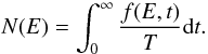$\mathit{N}\mathrm{\left(}\mathit{E}\mathrm{\right)}\mathrm{=}{\mathrm{\int }}_{\mathrm{0}}^{\mathrm{\infty }}\frac{\mathit{f}\mathrm{\left(}\mathit{E,t}\mathrm{\right)}}{\mathit{T}}\mathrm{d}\mathit{t}\mathit{.}$(5)Using Eq. (4) yields the observable spectrum 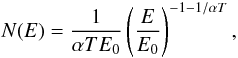$\mathit{N}\mathrm{\left(}\mathit{E}\mathrm{\right)}\mathrm{=}\frac{\mathrm{1}}{\mathit{\alpha T}{\mathit{E}}_{\mathrm{0}}}{\left(\frac{\mathit{E}}{{\mathit{E}}_{\mathrm{0}}}\right)}^{\mathrm{-}\mathrm{1}\mathrm{-}\mathrm{1}\mathit{/}\mathit{\alpha T}}\mathit{,}$(6)which coincides with a steady solution of Eq. (1). This is unsurprising since the first term in Eq. (1) vanishes when it is integrated with respect to time from 0 to ∞. Consequently if α = const., then N(E) is given by a steady solution to Eq. (1). This simple solution clearly shows that the observable spectrum N(E) outside the reservoir differs from the particle distribution f(E,t) inside the reservoir at any time, even though the escape time T = const. (see also Syrovatskii 1961).

The acceleration rate is determined by the energy density in the turbulence (Kulsrud & Ferrari 1971; see also Miller et al. 1990, and references therein). Following Burn (1975), assume that the acceleration efficiency α is proportional to the turbulent energy density W_t: $\mathit{\alpha }\mathrm{=}{\mathit{\alpha }}_{\mathrm{0}}\frac{{\mathit{W}}_{\mathrm{t}}}{{\mathit{n}}_{\mathrm{0}}{\mathit{E}}_{\mathrm{0}}}\mathit{,}$(7)where α₀ is a constant (cf. Achterberg 1979). Recall that the steady solution in Burn (1975) was derived by assuming a constant ratio of the injection rates of the turbulent energy and the particle energy into the reservoir. An analogous assumption in the present time-dependent formulation is that the ratio of the turbulent to particle energy densities (W_t and W_p) within the reservoir does not vary throughout the acceleration process: W_t/W_p = const. where ${\mathit{W}}_{\mathrm{p}}\mathrm{=}{{}^{\mathrm{\int }}}_{\mathrm{0}}^{\mathrm{\infty }}\mathit{f}\mathrm{\left(}\mathit{E,t}\mathrm{\right)}\mathit{E}\mathrm{d}\mathit{E}$. Parker (1958, 1969) discussed how such a balance could be established physically.

It would be desirable to have a concrete argument for the assumed balance W_t ~ W_p, based on quasilinear plasma theory (e.g., Achterberg 1979). The key point in the present context, however, is that the assumption of such a balance is equivalent to assuming that both the particle escape from the reservoir and the turbulent energy decay occur on the same timescale. This is consistent with the notion that the turbulence that accelerates particles in solar flares also traps them in the acceleration region (e.g., Smith et al. 1990). Since Burn (1975) considered a steady case of acceleration in a Fermi reservoir, the present paper and Burn (1975) analyse the opposite limiting cases of the problem. An intermediate case is likely to be realised in practice, yet it seems reasonable that exploration of the limiting cases can be a useful guide to the general problem.

On replacing W_t by W_p in Eq. (7), the acceleration efficiency is related to the particle distribution within the reservoir: $\mathit{\alpha }\mathrm{\left(}\mathit{t}\mathrm{\right)}\mathrm{=}\frac{{\mathit{\alpha }}_{\mathrm{0}}}{{\mathit{n}}_{\mathrm{0}}{\mathit{E}}_{\mathrm{0}}}{\mathrm{\int }}_{\mathrm{0}}^{\mathrm{\infty }}\mathit{f}\mathrm{\left(}\mathit{E,t}\mathrm{\right)}\mathit{E}\mathrm{d}\mathit{E}\mathit{.}$(8)It can be assumed without any loss of generality that W_t = W_p, because a proportionality constant can be absorbed into the definition of α₀. Substitution of Eq. (8) into (1) would give a single integro-differential equation for the particle distribution f(E,t) with parameters n₀, E₀, α₀, and T. As before, the initial condition is given by Eq. (2).

3. Solution

The above-formulated problem admits an exact analytical solution. First, the initial value problem, specified by Eqs. (1) and (2), is solved for an arbitrary α(t). A straightforward generalisation of Eq. (4) is $\mathit{f}\mathrm{\left(}\mathit{E,t}\mathrm{\right)}\mathrm{=}{\mathit{n}}_{\mathrm{0}}{\mathrm{e}}^{\mathrm{-}\mathit{t}\mathit{/}\mathit{T}}\mathit{\delta }\left(\mathit{E}\mathrm{-}{\mathit{E}}_{\mathrm{0}}{\mathrm{e}}^{\mathit{\tau }}\right)\mathit{,}$(9)where $\mathit{\tau }\mathrm{=}{{}^{\mathrm{\int }}}_{\mathrm{0}}^{\mathit{t}}\mathit{\alpha }\mathrm{\left(}{\mathit{t}}^{\mathrm{\prime }}\mathrm{\right)}\mathrm{d}{\mathit{t}}^{\mathrm{\prime }}$.

Next f(E,t) is substituted into Eq. (8). On evaluating the integral over E, Eq. (8) becomes $\mathit{\alpha }\mathrm{\left(}\mathit{t}\mathrm{\right)}\mathrm{=}{\mathit{\alpha }}_{\mathrm{0}}{\mathrm{e}}^{\mathit{\tau }\mathrm{-}\mathit{t}\mathit{/}\mathit{T}}\mathit{.}$(10)Differentiation with respect to time leads to the ordinary differential equation $\frac{\mathrm{d}\mathit{\alpha }}{\mathrm{d}\mathit{t}}\mathrm{=}\left(\mathit{\alpha }\mathrm{-}\frac{\mathrm{1}}{\mathit{T}}\right)\mathit{\alpha }\mathit{.}$(11)Alternatively, this energy balance equation follows from Eq. (1) on multiplying it by E, integrating over energy, and using Eq. (8). Equation (11) with an initial condition α(0) = α₀ is integrated to give $\mathit{\alpha }\mathrm{\left(}\mathit{t}\mathrm{\right)}\mathrm{=}{\left[\mathit{T}\mathrm{+}\left(\frac{\mathrm{1}}{{\mathit{\alpha }}_{\mathrm{0}}}\mathrm{-}\mathit{T}\right){\mathrm{e}}^{\mathit{t}\mathit{/}\mathit{T}}\right]}^{-1}\mathit{.}$(12)Here it is necessary to assume that α₀T < 1 to make sure that α(t), as well as the total particle energy, remains finite.

The observable spectrum outside the reservoir is obtained by substituting Eqs. (9) and (12) into (5) and integrating over time. The result is a power law 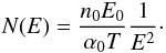$\mathit{N}\mathrm{\left(}\mathit{E}\mathrm{\right)}\mathrm{=}\frac{{\mathit{n}}_{\mathrm{0}}{\mathit{E}}_{\mathrm{0}}}{{\mathit{\alpha }}_{\mathrm{0}}\mathit{T}}\frac{\mathrm{1}}{{\mathit{E}}^{\mathrm{2}}}\mathrm{·}$(13)A notable feature of the solution is that the predicted spectral slope γ = 2 is independent of the parameters of the model. In the original Fermi model, this spectrum could only arise if by coincidence αT = 1. It is also worth emphasising that in a steady solution with an energy balance constraint, the particles leaving the reservoir and those contained within it have the same spectral index (Burn 1975). The picture is very different in the present time-dependent model. The observed particle spectrum N(E) outside the acceleration region clearly cannot be predicted from the distribution within the reservoir at any given time.

The spectrum N(E) is characterised by an upper energy cutoff. The energy per particle inside the reservoir is E(t) = E₀exp(^∫αdt), where α(t) is given by Eq. (12). Therefore, $\mathit{E}\mathrm{\left(}\mathit{t}\mathrm{\right)}\mathrm{=}{\mathrm{[}\mathrm{(}\mathrm{1}\mathrm{-}{\mathit{\alpha }}_{\mathrm{0}}{\mathit{T}}^{\mathrm{)}}\mathrm{+}{\mathit{\alpha }}_{\mathrm{0}}\mathit{T}{\mathrm{e}}^{\mathrm{-}\mathit{t}\mathit{/}\mathit{T}}\mathrm{]}}^{-1}{\mathit{E}}_{\mathrm{0}}\mathit{.}$(14)The maximum particle energy E₁ is calculated by taking the limit t → ∞: ${\mathit{E}}_{\mathrm{1}}\mathrm{=}{\mathrm{(}\mathrm{1}\mathrm{-}{\mathit{\alpha }}_{\mathrm{0}}{\mathit{T}}^{\mathrm{)}}}^{-1}{\mathit{E}}_{\mathrm{0}}\mathit{.}$(15)Hence, the total energy in the accelerated particles is given by ${\mathrm{\int }}_{{\mathit{E}}_{\mathrm{0}}}^{{\mathit{E}}_{\mathrm{1}}}\mathit{N}\mathrm{\left(}\mathit{E}\mathrm{\right)}\mathit{E}\mathrm{d}\mathit{E}\mathrm{=}\frac{{\mathit{n}}_{\mathrm{0}}{\mathit{E}}_{\mathrm{0}}}{{\mathit{\alpha }}_{\mathrm{0}}\mathit{T}}\ln \left(\frac{\mathrm{1}}{\mathrm{1}\mathrm{-}{\mathit{\alpha }}_{\mathrm{0}}\mathit{T}}\right)\mathrm{·}$(16)As a check of the calculation, observe that N(E) and E₁ satisfy the particle conservation equation 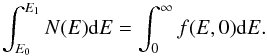${\mathrm{\int }}_{{\mathit{E}}_{\mathrm{0}}}^{{\mathit{E}}_{\mathrm{1}}}\mathit{N}\mathrm{\left(}\mathit{E}\mathrm{\right)}\mathrm{d}\mathit{E}\mathrm{=}{\mathrm{\int }}_{\mathrm{0}}^{\mathrm{\infty }}\mathit{f}\mathrm{\left(}\mathit{E,}\mathrm{0}\mathrm{\right)}\mathrm{d}\mathit{E}\mathit{.}$(17)A more general problem can also be solved analytically. Suppose that the acceleration efficiency is given by $\mathit{\alpha }\mathrm{=}{\mathit{\alpha }}_{\mathrm{0}}{\left(\frac{{\mathit{W}}_{\mathrm{t}}}{{\mathit{n}}_{\mathrm{0}}{\mathit{E}}_{\mathrm{0}}}\right)}^{\mathit{\kappa }}$(18)where κ > 0. Equation (18) reduces to Eq. (7) when κ = 1. The same steps as before lead to the following results. The acceleration efficiency as a function of time is $\mathit{\alpha }\mathrm{\left(}\mathit{t}\mathrm{\right)}\mathrm{=}{\left[\mathit{T}\mathrm{+}\left(\frac{\mathrm{1}}{{\mathit{\alpha }}_{\mathrm{0}}}\mathrm{-}\mathit{T}\right){\mathrm{e}}^{\mathit{\kappa t}\mathit{/}\mathit{T}}\right]}^{-1}\mathit{,}$(19)which generalises Eq. (12), the spectrum outside the reservoir is $\mathit{N}\mathrm{\left(}\mathit{E}\mathrm{\right)}\mathrm{=}\frac{{\mathit{n}}_{\mathrm{0}}{\mathit{E}}_{\mathrm{0}}}{{\mathit{\alpha }}_{\mathrm{0}}\mathit{T}}\frac{\mathrm{1}}{{\mathit{E}}^{\mathrm{2}}}{\left[\frac{\mathrm{1}}{{\mathit{\alpha }}_{\mathrm{0}}\mathit{T}}\mathrm{-}\left(\frac{\mathrm{1}}{{\mathit{\alpha }}_{\mathrm{0}}\mathit{T}}\mathrm{-}\mathrm{1}\right){\left(\frac{\mathit{E}}{{\mathit{E}}_{\mathrm{0}}}\right)}^{\mathit{\kappa }}\right]}^{\mathrm{-}\mathrm{1}\mathrm{+}\mathrm{1}\mathit{/}\mathit{\kappa }}\mathit{,}$(20)which generalises Eq. (13), and the maximum particle energy is ${\mathit{E}}_{\mathrm{1}}\mathrm{=}{\mathrm{(}\mathrm{1}\mathrm{-}{\mathit{\alpha }}_{\mathrm{0}}{\mathit{T}}^{\mathrm{)}}}^{\mathrm{-}\mathrm{1}\mathit{/}\mathit{\kappa }}{\mathit{E}}_{\mathrm{0}}\mathit{,}$(21)which generalises Eq. (15). Therefore, independently of the value of κ, the spectrum N(E) is characterised by the spectral index γ = 2 for sufficiently low energies. Near the upper energy cutoff E₁, however, the spectral shape is controlled by κ, so that N(E) → 0 as E → E₁ for κ < 1, whereas N(E) → ∞ as E → E₁ for κ > 1. Equation (17) is of course satisfied for any κ. A concrete model of turbulent wave-particle interaction would be needed to specify κ and to evaluate the physical significance of the results for κ ≠ 1.

While the maximum energy gain of Eq. (15) is quite modest if α₀T ≪ 1, the significance of the calculation is that it shows how a steady power-law spectrum of the type postulated by Burn (1975) could originate. Higher energies will be achieved if the particles experience several successive acceleration pulses. For κ = 1, the solution for each pulse is a generalisation of Eq. (13): $\mathit{N}\mathrm{\left(}\mathit{E}\mathrm{\right)}\mathrm{=}\frac{\mathrm{1}}{{\mathit{\alpha }}_{\mathrm{0}}\mathit{T}{\mathit{E}}^{\mathrm{2}}}{\mathrm{\int }}_{\left(\mathrm{1}\mathrm{-}{\mathit{\alpha }}_{\mathrm{0}}\mathit{T}\right)\mathit{E}}^{\mathit{E}}\mathit{F}\mathrm{\left(}\mathit{u}\mathrm{\right)}\mathit{u}\mathrm{d}\mathit{u,}$(22)where the initial spectrum F(E) in the reservoir is determined by the previous acceleration pulse.

4. Stochastic acceleration

The original formulation of stochastic acceleration (Fermi 1949) neglects the diffusive aspect of the process. More accurately, the evolution of the particle distribution f(E,t) is governed by 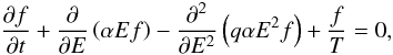$\frac{\mathit{\partial f}}{\mathit{\partial t}}\mathrm{+}\frac{\mathit{\partial }}{\mathit{\partial E}}\left(\mathit{\alpha Ef}\right)\mathrm{-}\frac{{\mathit{\partial }}^{\mathrm{2}}}{\mathit{\partial }{\mathit{E}}^{\mathrm{2}}}\mathrm{(}\mathit{q\alpha }{\mathit{E}}^{\mathrm{2}}{\mathit{f}}^{\mathrm{)}}\mathrm{+}\frac{\mathit{f}}{\mathit{T}}\mathrm{=}\mathrm{0}\mathit{,}$(23)where the third term describes stochastic fluctuations in energy (Davis 1956; Tverskoi 1967; Ball et al. 1992). The general form of the Fermi-acceleration momentum-diffusion coefficient leads to q = 1/4 in three dimensions (e.g., Miller et al. 1990, and references therein), but it is useful to treat q ≥ 0 as a parameter that quantifies the role of energy diffusion. Time-dependent stochastic acceleration in a Fermi reservoir is described by Eq. (23), which replaces Eq. (1), together with Eqs. (2) and (8).

Burn (1975) demonstrated analytically that the key predictions of the steady model remain unaltered when diffusion in energy is taken into account. Stochastic acceleration can be treated analytically in the present time-dependent model as well.

The solution of Eq. (23) with the initial condition specified by Eq. (2) is given by the Green’s function $\begin{array}{ccc}\mathit{G}\mathrm{(}\mathit{E,}{\mathit{E}}_{\mathrm{0}}\mathit{,}{\mathit{t}}^{\mathrm{)}}& \mathrm{=}& \frac{{\mathit{n}}_{\mathrm{0}}}{\mathrm{(}\mathrm{4}\mathit{\pi q\tau }{\mathrm{)}}^{\mathrm{1}\mathit{/}\mathrm{2}}\mathit{E}}{\left(\frac{\mathit{E}}{{\mathit{E}}_{\mathrm{0}}}\right)}^{\mathrm{(}\mathrm{1}\mathrm{-}\mathit{q}\mathrm{)}\mathit{/}\mathrm{2}\mathit{q}}\\ & & \end{array}$(24)This is a generalisation of Eq. (22) in Cowsik (1979). The result is most easily obtained by transforming Eq. (23) into the diffusion equation g_τ = qg_ξξ in the variables τ, ξ = ln(E/E₀), and g(ξ,τ) = exp [t/T + (1 − q)²τ/4q + (3q − 1)ξ/2q] f. In the limit q → 0, Eq. (24) reduces to Eq. (9).

Equations (11) and (12) remain valid for any q since diffusion in energy does not change the total energy in the reservoir. As in the basic model with q = 0, the spectrum of particles leaving the reservoir is obtained by substituting Eq. (24) into (5). The resulting integral can be expressed as $\begin{array}{ccc}\mathit{N}\mathrm{\left(}\mathit{E}\mathrm{\right)}& \mathrm{=}& \frac{\mathrm{2}}{\mathrm{(}\mathrm{1}\mathrm{+}\mathit{q}\mathrm{)}\sqrt{\mathit{\pi }}}\frac{{\mathit{n}}_{\mathrm{0}}}{{\mathit{\alpha }}_{\mathrm{0}}\mathit{TE}}{\left(\frac{\mathit{E}}{{\mathit{E}}_{\mathrm{0}}}\right)}^{\mathrm{(}\mathrm{1}\mathrm{-}\mathit{q}\mathrm{)}\mathit{/}\mathrm{2}\mathit{q}}\\ & & \end{array}$(25)where the upper integration limit ${\mathit{u}}_{\mathrm{1}}\mathrm{=}\frac{\mathrm{1}\mathrm{+}\mathit{q}}{\mathrm{2}}\sqrt{\frac{\mathrm{-}\ln \mathrm{(}\mathrm{1}\mathrm{-}{\mathit{\alpha }}_{\mathrm{0}}{\mathit{T}}^{\mathrm{)}}}{\mathit{q}}}\mathrm{·}$(26)In the limit q → 0, Eq. (25) reduces to Eq. (13).

Figure 1 shows both the analytical solution of Eq. (13) and a numerically evaluated solution for stochastic acceleration (Eq. (25) with q = 1/4). It is clear that diffusion in energy leads to particles with energies E < E₀ and E > E₁. The solution with q = 0 is a good predictor of the spectral slope in the range E₀ < E < E₁, except near the high-energy cutoff E₁ where the stochastic effects cause the spectrum to steepen.

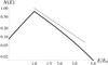Fig. 1 Particle spectrum N(E) outside a Fermi reservoir in an illustrative case α0T = 3/4. The thin upper line is the analytical scaling N(E) ~ E-2, predicted by Eq. (13) in the range 1 ≤ E/E0 ≤ 4 for regular Fermi acceleration (q = 0). The lower curve is the numerically evaluated stochastic acceleration solution of Eq. (25) with the parameter q = 1/4 that corresponds to Fermi acceleration in three dimensions.

5. Discussion

The differential energy spectrum of accelerated particles N(E)  ~  E^-2 appears to be consistent with a minimum value of the spectral index of energetic electrons, which can be deduced from the hard X-ray and gamma-ray observations in some impulsive solar flares (Rieger et al. 1998; Holman et al. 2003). Although the observed spectrum can vary significantly during a flare and from flare to flare, some electron-rich flares are characterised by a “soft-hard-harder” pattern of spectral evolution (e.g., Hudson & Fárník 2002), and the minimum observed value of the spectral index presumably identifies a pure spectrum of flare-accelerated electrons, that is isolated from a thermal background.

More speculatively, since source ion spectra of galactic cosmic rays are typically characterised by a spectral index γ ≈ 2 (Swordy 2001), the main argument of this paper may be of more general astrophysical relevance. Although diffusive shock acceleration remains the most favoured cosmic-ray acceleration mechanism (Axford 1981), there is currently renewed interest in applying a stochastic mechanism to Galactic cosmic rays (Fisk & Gloeckler 2012).

It is of interest to note an alternative approach to the problem of a power-law spectrum formation. Suppose that the particle kinetic energy inside a reservoir remains a constant fraction δ of the remaining (say, turbulent plus magnetic) energy in the reservoir. A general argument, independent of a specific acceleration mechanism, leads to a power-law spectrum N(E) ~ E^{−2 − δ} of the particles escaping from the reservoir (Syrovatskii 1961). The difference from the present calculation is that here, as well as in Burn (1975), the particle energy is related to the turbulent energy rather than to the total energy of the system. In contrast, straightforward application of energy conservation, by allowing the turbulent energy density to decrease as the particle energy

density increases, results in almost flat spectra (γ ≲ 1) below a high-energy cutoff (Eichler 1979; MacKinnon 1991).

Some limitations of the arguments in this paper are worth noting. The discussion of Fermi acceleration was carried out in very general terms. In particular, no reference was made to specific wave modes. Nevertheless, any concrete physical model incorporating the ideas of Burn (1975) and this paper should explicitly describe turbulence in specific wave modes. This is important because different waves resonate with different types of particles. For instance, it was argued that Alfvén waves accelerate ions, whereas fast-mode waves accelerate electrons in solar flares (e.g., Miller & Roberts 1995; Emslie et al. 2004, and references therein). It is also important to remember that the assumption T = const. was made here for the sake of mathematical simplicity. Physical considerations suggest, however, that the particle escape time is a function of energy (e.g., Pikelner & Tsytovich 1976; Smith et al. 1990). To achieve further progress in a model with a more realistic description of particle escape, it will probably be necessary to solve a time-dependent transport equation with T = T(E) numerically.

To sum up, this paper presents a simple time-dependent model for particle acceleration in a Fermi reservoir. The model complements the steady analysis in Burn (1975) and shows how a power-law spectrum of accelerated particles, similar to that postulated by Burn (1975), could form in the first place. Keeping in mind the limitations of the analytical model, the predicted spectrum of accelerated particles with a spectral index γ = 2 may be applicable in various astrophysical applications.

Acknowledgments

I thank Michael Wheatland (University of Sydney) for encouraging me to derive the stochastic acceleration Green’s function. I also acknowledge the referee whose detailed constructive report was very helpful.

References

All Figures

Fig. 1 Particle spectrum N(E) outside a Fermi reservoir in an illustrative case α0T = 3/4. The thin upper line is the analytical scaling N(E) ~ E-2, predicted by Eq. (13) in the range 1 ≤ E/E0 ≤ 4 for regular Fermi acceleration (q = 0). The lower curve is the numerically evaluated stochastic acceleration solution of Eq. (25) with the parameter q = 1/4 that corresponds to Fermi acceleration in three dimensions.

In the text

References

- Achterberg, A. 1979, A&A, 76, 276 [NASA ADS] [Google Scholar]
- Axford, W. I. 1981, Proc. 17th Int. Cosmic Ray Conf. (Paris), 12, 155 [NASA ADS] [Google Scholar]
- Ball, L., Melrose, D. B., & Norman, C. A. 1992, ApJ, 398, L65 [NASA ADS] [CrossRef] [Google Scholar]
- Burn, B. J. 1975, A&A, 45, 435 [NASA ADS] [Google Scholar]
- Cowsik, R. 1979, ApJ, 227, 856 [NASA ADS] [CrossRef] [Google Scholar]
- Davis, L. 1956, Phys. Rev., 101, 351 [NASA ADS] [CrossRef] [Google Scholar]
- Eichler, D. 1979, ApJ, 229, 413 [NASA ADS] [CrossRef] [Google Scholar]
- Emslie, A. G., Miller, J. A., & Brown, J. C. 2004, ApJ, 602, L69 [NASA ADS] [CrossRef] [Google Scholar]
- Fermi, E. 1949, Phys. Rev., 75, 1169 [NASA ADS] [CrossRef] [Google Scholar]
- Fermi, E. 1954, ApJ, 119, 1 [NASA ADS] [CrossRef] [Google Scholar]
- Fisk, L. A., & Gloeckler, G. 2012, ApJ, 744, 127 [Google Scholar]
- Ginzburg, V. L., & Syrovatskii, S. I. 1964, The Origin of Cosmic Rays (New York: Macmillan) [Google Scholar]
- Holman, G. D., Sui, L., Schwartz, R. A., & Emslie, A. G. 2003, ApJ, 595, L97 [NASA ADS] [CrossRef] [Google Scholar]
- Hudson, H. S., & Fárník, F. 2002, in Solar Variability: From Core to Outer Frontiers, ed. A. Wilson (Noordwijk: ESA Publications), ESA SP-506, 261 [Google Scholar]
- Kulsrud, R., & Ferrari, A. 1971, Ap&SS, 12, 302 [NASA ADS] [CrossRef] [Google Scholar]
- Lee, M. A. 1994, in High-Energy Solar Phenomena – A New Era of Spacecraft Measurements, eds. J. M. Ryan, & W. T. Vestrand, AIP Conf. Proc., 294, 134 [Google Scholar]
- Liu, C., & Wang, H. 2008, ApJ, 696, L27 [NASA ADS] [CrossRef] [Google Scholar]
- MacKinnon, A. L. 1991, Vistas Astron., 34, 331 [NASA ADS] [CrossRef] [Google Scholar]
- Miller, J. A., & Roberts, D. A. 1995, ApJ, 452, 912 [NASA ADS] [CrossRef] [Google Scholar]
- Miller, J. A., Guessoum, N., & Ramaty, R. 1990, ApJ, 361, 701 [NASA ADS] [CrossRef] [Google Scholar]
- Parker, E. N. 1958, Phys. Rev., 109, 1328 [NASA ADS] [CrossRef] [Google Scholar]
- Parker, E. N. 1969, Space Sci. Rev., 9, 651 [NASA ADS] [Google Scholar]
- Pikelner, S. B., & Tsytovich, V. N. 1976, Sov. Astron., 19, 450 [NASA ADS] [Google Scholar]
- Rieger, E., Gan, W. Q., & Marschhäuser, H. 1998, Sol. Phys., 183, 123 [NASA ADS] [CrossRef] [Google Scholar]
- Smith, D. F., Chambe, G., Henoux, J. C., & Tamres, D. 1990, ApJ, 358, 674 [NASA ADS] [CrossRef] [Google Scholar]
- Swordy, S. P. 2001, Space Sci. Rev., 99, 85 [NASA ADS] [CrossRef] [Google Scholar]
- Syrovatskii, S. I. 1961, Sov. Phys. JETP, 13, 1257 [Google Scholar]
- Tverskoi, B. A. 1967, Sov. Phys. JETP, 25, 317 [Google Scholar]
- Zhang, M., & Lee, M. A. 2012, Space Sci. Rev., in press [Google Scholar]