| Issue |
A&A
Volume 544, August 2012
|
|
|---|---|---|
| Article Number | A156 | |
| Number of page(s) | 11 | |
| Section | Cosmology (including clusters of galaxies) | |
| DOI | https://doi.org/10.1051/0004-6361/201219507 | |
| Published online | 24 August 2012 | |
UltraVISTA: a new ultra-deep near-infrared survey in COSMOS⋆,⋆⋆
1 Institut d’Astrophysique de Paris, UMR7095 CNRS, Université Pierre et Marie Curie, 98 bis Boulevard Arago, 75014 Paris, France
e-mail: This email address is being protected from spambots. You need JavaScript enabled to view it.
2 Dark Cosmology Centre, Niels Bohr Institute, University of Copenhagen, Juliane Maries Vej 30, 2100 Copenhagen, Denmark
3 SUPA, Institute for Astronomy, University of Edinburgh, Royal Observatory, Edinburgh, EH9 3 HJL, UK
4 Leiden Observatory, Leiden University, PO Box 9513, 2300 RA Leiden, The Netherlands
5 Laboratoire d’Astrophysique de Marseille, CNRS et Aix-Marseille Université, 38 rue Frédéric Joliot-Curie, 13388 Marseille Cedex 13, France
6 Kapteyn Astronomical Institute, University of Groningen, PO Box 800, 9700 AV Groningen, The Netherlands
7 Astronomy Unit, School of Physics and Astronomy, Queen Mary University of London, Mile End Road, London, E1 4NS, UK
8 European Southern Observatory, Karl-Schwarzschild-Strasse 2, 85748 Garching bei München, Germany
Received: 30 April 2012
Accepted: 22 June 2012
Abstract
In this paper we describe the first data release of the UltraVISTA near-infrared imaging survey of the COSMOS field. We summarise the key goals and design of the survey and provide a detailed description of our data reduction techniques. We provide stacked, sky-subtracted images in YJHKs and narrow-band filters constructed from data collected during the first year of UltraVISTA observations. Our stacked images reach 5σAB depths in an aperture of 2″ diameter of ~25 in Y and ~24 in JHKs bands and all have sub-arcsecond seeing. To this 5σ limit, our Ks catalogue contains 216 268 sources. We carry out a series of quality assessment tests on our images and catalogues, comparing our stacks with existing catalogues. The 1σ astrometric rms in both directions for stars selected with 17.0 < Ks(AB) < 19.5 is ~0.08″ in comparison to the publicly-available COSMOS ACS catalogues. Our images are resampled to the same pixel scale and tangent point as the publicly available COSMOS data and so may be easily used to generate multi-colour catalogues using this data. All images and catalogues presented in this paper are publicly available through ESO’s “phase 3” archiving and distribution system and from the UltraVISTA web site.
Key words: surveys / galaxies: general / galaxies: high-redshift / cosmology: observations / large-scale structure of Universe
Based on data products from observations made with ESO Telescopes at the La Silla Paranal Observatory under ESO programme ID 179.A-2005 and on data products produced by TERAPIX and the Cambridge Astronomy Survey Unit on behalf of the UltraVISTA consortium.
Catalogs are only available at the CDS via anonymous ftp to cdsarc.u-strasbg.fr (130.79.128.5) or via http://cdsarc.u-strasbg.fr/viz-bin/qcat?J/A+A/544/A156
© ESO, 2012
1. Introduction
The vital role of near-infrared (λ ≃ 1−2.5 μm) imaging surveys for advancing our understanding of galaxy evolution has long been recognised (Cowie et al. 1990; Glazebrook et al. 1991). While optical surveys utilising large-format charge-coupled device (CCD) detectors were the first to enable the discovery of substantial samples of normal galaxies at redshifts z > 2 (Steidel et al. 1996; Madau et al. 1996), it was already known that at least some galaxies at high redshift were either too old or too dust-obscured to be easily detected by rest-frame near-ultraviolet selection (Dunlop et al. 1996; Dey et al. 1996). In addition, even for apparently young UV-luminous galaxies, the value of using near-infrared observations to sample the rest-frame optical light, more representative of the evolved mass-dominant stellar population, was understood and indeed demonstrated before the advent of multi-pixel near-infrared imagers (Lilly & Longair 1984).
However, near-infrared surveys are a challenging proposition for several reasons. Firstly, at near-infrared bandpasses the sky background is extremely bright; in the Ks band, in AB magnitudes, it is typically 15 mag/arcsec2, which means that many short exposures must be combined in order to avoid detector saturation on the sky, greatly increasing overheads. Secondly, the sky background is time-variable, many magnitudes brighter than the faint astronomical sources of interest, and so must be carefully subtracted from each image before scientific exploitation can take place. Lastly, conventional silicon CCDs are very inefficient at near-infrared wavelengths, and a different detector technology must be employed which is an order of magnitude more expensive. In terms of sky footprint, near-infrared detectors have generally lagged behind optical detectors by approximately a decade.
Nevertheless, these challenges have been progressively overcome, and, following the pioneering work described above with early near-infrared arrays such as IRCAM on the UK Infrared Telescope (UKIRT; McLean et al. 1986), the full potential of near-infrared surveys to clarify our view of galaxy evolution at z ≃ 1 − 3 began to be realised with the advent of larger format infrared array cameras such as ISAAC on ESO’s Very Large Telescope (VLT; Cimatti et al. 2002; Labbé et al. 2003; Franx et al. 2003). Meanwhile, the importance of near-infrared surveys for revealing dust-obscured star-forming galaxies was further enhanced by the discovery of significant numbers of dusty-enshrouded high-redshift star-forming galaxies at sub-mm wavelengths (Hughes et al. 1998; Scott et al. 2002). Around the same time the unique power of the deepest near-infrared imaging to conduct rest-frame ultraviolet surveys for galaxies at z > 6.5 was first demonstrated using the NICMOS camera on the Hubble Space Telescope (HST; Bouwens et al. 2004; Thompson et al. 2005).
Despite these impressive advances, the field-of-view offered by near-infrared cameras such as IRCAM, NICMOS and ISAAC was very small (a few arcmin2), and it is only in the last half-decade or so that the introduction of genuinely large-format near-infrared array cameras has enabled efficient, deep near-infrared imaging of degree-scale areas of sky, allowing studies of more representative volumes of the high-redshift universe (i.e. ≃ 100 × 100 comoving Mpc). First WFCAM on UKIRT (Casali et al. 2007), then WIRCam on the Canada France Hawaii Telescope (CFHT; Puget et al. 2004), and NEWFIRM at NOAO (Probst 2004) have heralded a new era of major coordinated near-infrared survey programmes (e.g. UKIDSS, Lawrence et al. 2007; NEWFIRM Medium-Band Survey, van Dokkum et al. 2009); WIRDS and associated near-infrared follow-up of the COSMOS field (Bielby et al. 2012; McCracken et al. 2010). This has led to a number of breakthroughs in extra-galactic astronomy, including, for example, the study of the bright end of the galaxy luminosity function from z = 0 out to z ≃ 6 (McLure et al. 2009; Cirasuolo et al. 2010), and the discovery of the most distant known quasar (Mortlock et al. 2011).
In addition, deep, wide-field near-infrared photometry coupled with high-quality optical surveys has enabled spectral energy distribution (SED) fitting techniques to be pushed beyond z ~ 1.5. Near-infrared data play a key role in minimising the catastrophic failure rates in photometric redshift estimates and provides robust rest-frame visible flux determinations at z ~ 2 (Ilbert et al. 2009), enabling measurements of the evolution of the mass buildup in stars over a large fraction of the age of the Universe (Drory et al. 2005; Arnouts et al. 2007; Ilbert et al. 2010; Caputi et al. 2011).
These efforts have now culminated in VISTA (Emerson & Sutherland 2010) the first 4-m class telescope specifically designed to conduct wide-area near-infrared surveys and equipped with a large-format array camera, “VIRCAM” (Dalton 2006). Thanks to its large mosaic of 16 detectors, VIRCAM is currently the most efficient wide-field near-infrared survey camera in the world (around four times more efficient than WIRCam, and three times as efficient as WFCAM). It also has the benefit of being mounted on a telescope for which virtually all observing time is available for surveys, and for which observations are efficiently programmed in queue-scheduled mode. Inspired by the success of UKIDSS, ESO has implemented a coordinated multi-tier public survey programme with VISTA. The UltraVISTA survey presented here is the deepest component of the VISTA survey “wedding cake”.
Covering an area of 1.5 deg2, UltraVISTA is significantly larger than the only comparably-deep near-infrared survey conducted to date (the UKIDSS Ultra Deep Survey UDS; Almaini et al. 2007), and will ultimately go significantly deeper. VIRCAM also offers two significant advantages over WFCAM (and indeed WIRCam or NEWFIRM) in that its Raytheon detectors are much more sensitive in Y-band, and are essentially free from the electronic cross-talk. These are crucial benefits in the planned exploitation of UltraVISTA for the discovery of the most luminous galaxies at z ≃ 7, e.g., Bowler et al. (2012).
To maximise the leverage and legacy value of these new deep near-infrared data, the UltraVISTA survey is centred on the COSMOS field, the location of the largest ever ACS optical mosaic obtained with HST (Scoville et al. 2007; Koekemoer et al. 2007) and an ever growing heritage of deepground-based and space-based multi-frequency imaging and spectroscopy1 . The first-year data set described in this paper is already deeper than all existing COSMOS NIR data (McCracken et al. 2010; Bielby et al. 2012) in all bands by between one and two magnitudes and also contains for the first time deep Y-band imaging.
To most efficiently exploit VISTA for the discovery and study of UV-selected galaxies at the highest redshifts (z ≃ 6.5 − 9) and in the investigation of the growth of galaxies through the crucial redshift range 1 < z < 3 when cosmic star-formation density peaks (Hopkins & Beacom 2006), the UltraVISTA survey comprises three separate components: a wide, deep Y,J,H,Ks survey (a contiguous field covering ≃ 1.5 deg2); an ultra-deep Y,J,H,Ks survey (consisting of deeper strips covering ≃ 0.7 deg2), and an ultra-deep narrow-band (λ = 1.18 μm) survey targeting emission-line galaxies at a range of redshifts, e.g. Hα at z = 0.8, [OIII]-emitters at z = 1.4, [OII] emitters at z = 2.2, and ultimately Lyα emitters at z = 8.8. To accomplish these goals, UltraVISTA has been allocated 1800 h of execution time.
It is important to stress that while the advent of Wide Field Camera 3 (WFC3) on HST in 2009 has enabled extremely deep near-infrared imaging (up to λ ≃ 1.6 μm) which has revolutionised the study of galaxies at z ≃ 7−8, (Bouwens et al. 2010; McLure et al. 2010; Oesch et al. 2009; Finkelstein et al. 2010; Bunker et al. 2010) the very small field-of-view offered by WFC3/IR coupled with its inability to observe in the K-band means that deep ground-based surveys such as UltraVISTA remain of crucial importance. In particular, the largest current (or indeed planned) WFC3/IR extragalactic survey is the Cosmic Assembly Near-infrared Deep Extragalactic Legacy Survey (CANDELS; Grogin et al. 2011; Koekemoer et al. 2011), but even this 900-orbit 3-year HST Treasury Program will only cover ≃ 800 arcmin2. Thus UltraVISTA is an excellent complement to CANDELS, and indeed CANDELS has recently completed deep J,H-band WFC3/IR imaging of a ≃200 arcmin2 region within the 1.5 deg2 UltraVISTA imaging described here (i.e. covering only ≃4% of UltraVISTA).
In this paper we present a detailed description of the data reduction methods and properties of the five near-infrared stacks created from the first season of UltraVISTA operations. Already, with only these first images, the UltraVISTA survey has the largest étendue of any near-infrared survey.
All magnitudes in this paper, unless otherwise noted, are given in the AB system. Data products described here are available fromESO2 ,the UltraVISTA website3andCESAM4 .
Characteristics of the OBs used in UltraVISTA season 1.
2. Observations and data reductions
2.1. Observations
The images described here were taken between 5th December 2009 and the 19th of April 2010 with the VIRCAM instrument on the VISTA telescope at Paranal as part of the UltraVISTA survey programme. VIRCAM is a wide-field near-infrared camera consisting of 16 2048 × 2048 Raytheon VIRGO HgCdTe arrays arranged in a sparse-filled array with gaps between each array of 0.90 & 0.425 of a detector in X and Y respectively (Emerson & Sutherland 2010). The mean pixel scale is 0.34″ pixel-1 (Dalton 2006).
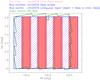 |
Fig. 1 Schematic layout of UltraVISTA observations, showing deep and ultra-deep regions (hatched and filled regions respectively). The data described in this paper correspond to a uniform coverage in YJHKs of the contiguous region and to NB118 observations of the ultra-deep stripes. |
The sky coverage of the 16 non-contiguous detectors is called a “pawprint”. A contiguous region of size 1.5° × 1.23° can be covered by means of six pawprints suitably spaced in right ascension and declination with random 60″ jitter offsets in both directions (two ≈ 0.1° bands at the top and bottom of the field receive half the exposure time).
Specifically, three pawprints with identical RA and with Dec differing by 5.5′ = 47.5% of a detector height make up a set of four stripes (corresponding to the ultra-deep stripes in UltraVISTA), and another three pawprints shifted by 95% of a detector width in RA make up another set of stripes, which together form a contiguous region where most pixels in the resulting stack are covered by two of the six pawprints.
Figure 1 illustrates the layout of UltraVISTA observations showing the deep survey, which will cover the full survey area, and the ultra-deep part, which covers half of this area in a series of ultra-deep stripes. The first season of UltraVISTA data described in this paper comprises six contiguous pawprints in four broad-band filters covering the deep survey area, each with equal exposure times, and narrow band observations on the ultra-deep stripes; subsequent observing seasons are expected to concentrate exclusively on the ultra-deep stripes.
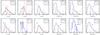 |
Fig. 2 Seeing (left) and ellipticity (right) distributions for all UltraVISTA images considered. The arrow represents the median of each distribution for images classified as A or AB. Note that the distributions for each quality class have been re-normalised, and the vertical axis has been rescaled. A, AB, C represent the quality classifications described in the text. |
The observations, carried out in service mode, are specified by observation blocks (OBs). The characteristics of the OBs used in UltraVISTA season one are listed in Table 1. Most of the season one OBs comprise images jittered around the centre of a single pawprint position, with the jitters being drawn from a random, uniform distribution over a box of side length 120′′ (random jitters are necessary because of persistence effects in VIRCAM and are also essential to derive a good sky frame).
The exception to this was the “NB118 three paws” OBs (Table 1), which comprised images jittered around the centres of the three pawprints forming the ultra-deep stripes. For OBs containing more than a single pawprint per OB, the nesting (Table 1) is important, and we did not use the optimal value. These OBs had a nesting of “FJPME” such that F (filter) is the outermost loop, and E (expose) is the innermost loop. The important aspect here is that the three pawprints (P) (spaced exactly by 5.5′ in Dec) are completed before a random jitter (J) is applied. This means that the faint persistent images (i.e. fake sources that are memories of a bright star at that x, y position on the detector in the one or two previous exposures) will be present in the stack at positions located 5.5′ (and 11′) away from bright stars in Dec. We deal with this by masking the persistent images in the individual NB118 images (see Milvang-Jensen et al., in prep., for details of the procedure). For the other UltraVISTA OBs, the faint persistent images are fully removed by the sigma clipping used in producing the stacks, thanks to the random jitters applied between each single exposure. The first season of observations described here comprise around 200 OBs in total. The average efficiency (calculated as the total exposure time divided by total execution time these OBs) was 77%.
In light of our experience gained in the season one observations described here, from season 2 onwards we modified some of the OBs. For Y, we changed the DIT to 60 s (with NDIT = 2), since 30 s was unnecessarily short; for H, we changed the DIT to 10 s (with NDIT = 6), for the same reason. For NB118, we changed the DIT to 120 s (with NDIT = 1), since 300 s was unnecessarily long. We also changed our observation strategy to jitters centered around a single pawprint per OB, and changed the total exposure time per OB to 1 h (corresponding to 30 jittered exposures in an OB).
2.2. Image selection and grading
VIRCAM images are transferred to the Cambridge Astronomy Survey Unit(CASU)5for pre-preprocessing and removal of the instrumental signature. This includes dark subtraction, correction for rest anomaly, flat-fielding, initial sky-subtraction, de-striping, non-linearity corrections and gain normalisation (Irwin et al. 2004). CASU subsequently provides these pre-processed images for each survey, as well as stacks of images from a single OB and pawprint, comprising typically 30 or 60 images.
For UltraVISTA we start from the individual pre-processed images, rather than the stacked OB blocks, for a number of reasons: firstly, the OB blocks are combined at CASU at the native pixel scale of the instrument, which means that in good seeing conditions (median FWHM ~ 0.6″) VIRCAM data is under-sampled. For this reason it is preferable to re-sample these data at a finer pixel scale; secondly, one of the principal scientific aims of the UltraVISTA project is to make measurements of distant (z > 6) and faint (Ks ≃ 24) galaxies. To do this requires extremely accurate removal of the sky background for each individual image; in the version of the CASU pipeline we used, a single sky background was used for all images coming from a given OB, and objects were not masked using the deepest possible mask. Given that the sky background is known to vary on shorter timescales, this process may lead to a systematic magnitude offset at faint magnitudes near bright sources. For these reasons we use an iterative sky-background removal technique starting from the pre-processed images and also resample all data to a pixel scale of 0.15″ pixel-1.
The images in this release were taken between 5th December 2009 and the 19th of April 2010. This does not consist of the complete number of images taken for the UltraVISTA program in the 2009–2010 observing season; subsequently, around 10% additional images in H and Ks were made available by CASU using a different pipeline processing, after we had already graded the first batch of images. In order to maintain as a homogenous as possible data set, we restrict in this release ourselves to this initial batch. However, had we included these data, the average exposure time per pixel would have been 4800 s and 5400 s higher in H and Ks respectively, i.e. only around 10% larger. The images considered here were all processed with v0.8 of the CASU pre-processing pipeline and in total, we consider 7031 individual images (each of which is a single multi-extension fits image containing 16 image extensions one for each of the VISTA detectors).
Since UltraVISTA represents the first significant amount of data from VIRCAM processed at TERAPIX, we wished to visually inspect all images to identify any problems which had been potentially overlooked by the automatic pipelines. Therefore, all images were inspected and graded in the YOUPI6 environment. Images were assigned a grade of A, B (usable for science), C, D (rejected). The left and right panels of Fig. 2 shows the seeing FWHM (measured assuming a Gaussian core), ellipticity and grading distributions for all images. Based on these distributions we decided to keep all images which have stellar FWHM < 1.0″ and ellipticity <0.1 and which were classified as either A or B based on visual inspection. The visual inspection process in general finds images which have bad point spread functions (PSFs) or other optical defects which would have not been found by a typical seeing or ellipticity cut7. In total we reject 426 images or around 6% of the total.
We do not use the confidence maps provided by CASU, but create our own weight maps from the supplied flat-fields and bad pixel maps using the weightwatcher tool (Marmo & Bertin 2008). For our NB118 images which were taken at a fixed set of jitter patterns and thus suffer from image persistence effects, we mask the persistent images using the procedure described in Milvang-Jensen et al. (in prep.).
2.3. Two-step sky subtraction
To derive our sky-subtracted images, we use a set of tools developed at TERAPIX which run under the distributed processing environment “condor”8. (These processing steps are described fully in Bielby et al. 2012). Sky-subtraction is a two-step iterative process. To summarise, we start by adding back the sky background frames subtracted by CASU (which are supplied as part of the original data release.) Based on the first-pass stack (computed using the CASU sky-subtracted images) and astrometric solutions, we compute object masks for each individual image. Next, we use these object masks (appropriately resampled based on an initial astrometric solution) to effectively remove objects computed from a running sky for each individual image, based on a median of images taken during a 20-min sliding window. After the subtraction of the running sky, we re-“destripe” the images and remove large-scale background gradients using sextractor (Bertin & Arnouts 1996). In general, computing sky backgrounds for each of the 7000 images is highly processor intensive; for each image, it takes around 15–20 min on a standard TERAPIX computing node.
2.4. Astrometric and photometric solutions
After sky-subtraction, weight maps and catalogues are computed once more for each image using QualityFITS. Saturated objects, based on an examination of the distribution of objects in the peak surface brightness/magnitude plane, are flagged in these catalogues, and the weight maps are used to flag cosmic rays. Bad pixels are also flagged. Next, these catalogues are used to compute the final astrometric and photometric solutions which will be used to combine and scale the images. Astrometric solutions are computed independently from each filter using the scamp tool (Bertin 2006), but use a common astrometric reference catalogue drawn from the COSMOS i-band CFHT data (the same reference catalogue used in Capak et al. 2007; McCracken et al. 2010). We use a third-order polynomial solution in x and y detector co-ordinates (note that unlike the CASU reductions, we do not assume a radially symmetric astrometric solution). In order to derive a more robust astrometric solution, we use a precomputed “.ahead” file for all images which specifies the relative positions and orientations of each of the sixteen detectors. In addition, we require that all the detectors share a common tangent point (focal plane mode “SAME_CRVAL” in scamp). These steps ensure that we can reliably match our reference astrometric catalogues for many thousands of input images (note that we do not use the higher-order terms of the initial astrometric solution provided byCASU9 ). Thanks to our densely sampled astrometric reference catalogue the internal sigma of our astrometric solution is ~0.08″,0.09″ in directions North-South, East-West directions respectively.
Compared to our reference catalogue, in the same directions, we find standard deviations of ~0.09″,0.10″. Similar values are found in all filters. Given that the native pixel scale of VIRCAM is 0.34″ pixel-1, our astrometric solution is more than sufficient to provide a precise and reliable image coaddition (in fact, our astrometric accuracy is probably limited by undersampling in the VIRCAM images).
Our initial magnitude zero points for each individual image are based on those supplied by CASU for their .st stacks (which comprise a stack of several individual images), which is based on their calibration of the VISTA photometric system’s zero points. To account for possible photometric variations between the images in each .st stack we calculate a rescaling factor for each using scamp based on overlapping paw-prints. Note that the same rescaling factors are applied to all detectors: we assume that the relative scaling factors between chips does not change (the CASU processing pipeline equalises the gain between all detectors at the flat-fielding stage, and should remain constant). To create our final stacks in the AB magnitude system (Oke 1974) we simply apply the appropriate flux scaling to convert the supplied Vega magnitudes to AB, based on the VISTA telescope detector, filter and atmosphere combination. The conversion factor C from AB to Vega we use are as follows, in the sense magAB = magvega + C where C = 0.61,0.90,1.38,1.84,0.86 for Y,J,H,Ks and NB118 filters respectively.
Note that CASU produces “flat” images which have constant flux per pixel for a uniform illumination; this is taken into account in the resampling stage.
2.5. Coadded images
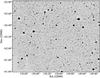 |
Fig. 3 Full Ks mosaic, displayed using a logarithmic stretch. The background level is extremely flat, and is not perturbed near almost all bright stars. Several clusters are visible, corresponding to the many rich structures which are present in the COSMOS field. |
Characteristics of the stacked images.
In the last processing step, the images and weight maps are coadded using a modified version of the swarp software (Bertin et al. 2002) which permits a combination of images based on a clipped sigma estimator; we use a clipping threshold of 2.8σ. Before stacking, a small number of images which have large photometric extinction or bad astrometric solutions are also rejected. For the final stacks, in the five bands, 6520 images were used. Since the size of VIRCAM pixels varies radially as a function of distance from the centre of the mosaic, this must be accounted for during image co-addition. Bad regions on individual detectors (such as half of detector 16, whose pixels suffer from time variable quantum efficiency, most notable at shorter wavelengths where the sky background is lower) are also masked, which explains the irregular appearance in the corner of the stacked images. Figure 3 shows most of the Ks image, resampled 2 × 2. The final image is completely free of any large-scale gradients, and the background is perfectly flat except near the brightest objects in the field.
In this release, five stacked images and their corresponding weight maps are made available for Y, J, H, Ks and NB118 data taken during the first year of public survey operations of the UltraVISTA survey. These images have a zero point of 30.0 AB magnitudes for an effective exposure time of one second and a pixel scale of 0.15″/pixel. The weight-maps correspond to swarp’s image type MAP_WEIGHT which correspond to maps of relative inverse variance. Figure 4 shows an RGB image composed KsJY images of a small section of the final field, illustrating the excellent image quality and depth of our final stacks. The bright saturation limit for stellar sources in these catalogues is ~14 mag in Y and 15 mag in YJHKs bands.
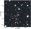 |
Fig. 4 RGB image composed of Ks, J and Y data respectively. The size of this image represents less than 1/500th of the total area of the field. Sources as faint as Ks ~ 22 are easily visible. |
The images all have a common tangent point, in decimal RA, Dec of (1.501163213, 2.200973097), corresponding to the tangent point of the publicly available IRSA/COSMOS images. Each image (uncompressed) is ~9 Gb in size. This common tangent point and pixel scale means that the UltraVISTA survey images are pixel-matched to publicly available COSMOS data.
Finally, to prepare these data products for ingestion in ESO’s “phase three” system, all the image and table headers produced were edited to comply with the Phase 3 requirement document, including most of the information which is presented here in the FITS header keywords.
Table 2 summarises the principal properties of each coadded stack. In each case we report the average seeing over the full mosaic, the 95% completeness limit, and the limiting magnitude. We also list the typical exposure time per pixel for each stack as well as the total on-sky integration time. Summed over all filters, this is 55 and 155 h respectively for the data presented here. Seeing on the final stack is characterised using the PSFex tool. The average seeing is calculated from a fit to a Moffat (1969) profile. We note that in Y band the PSF has slightly broader wings compared to redder bandpasses (with a best-fitting Moffat β parameter which varies from ~2.4 in Y to ~3.5 in Ks).
Limiting magnitudes are computed as follows: first, SEXtractor is run on each stack using the same detection threshold parameters as used for catalogue generation. All pixels belonging to objects to this detection limit are flagged. Next, we measure fluxes in apertures of diameter 2″ over the entire mosaic; any aperture which contains object pixels is discarded. The limiting magnitude is then simply computed from the standard deviation of fluxes measured in these apertures. Our completeness statistics are computed by adding artificial stars to the images with average image FWHM and then measuring the fraction which are successfully detected with SExtractor using the same measurement parameters used for the catalogues.
Figure 5 shows the weight-map from the first year of Ks observations described in this paper. The intensity at each pixel has been converted to an approximate limiting magnitude for a detection in a 5σ,2″ aperture. It is important to note that our weight map is quite uniform, thanks to our adopted observing strategy.
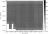 |
Fig. 5 Weight-map for the first-year Ks-band data. The intensity at each pixel has been converted to an approximate 5σ limiting magnitude for an aperture of 2″ diameter. The strips at the top and bottom of the image have half the average exposure time per pixel. |
From these stacks, two sets of catalogues are provided at the ESO archive: those extracted on individual images, and matched catalogues which use the Ks band image as a detection image. Aperture magnitudes reported in the catalogues are measured in 2″ and 7.1″ diameters respectively. Based on the average stellar profiles each of the four broad-band filters, these aperture magnitudes can be “corrected” to pseudo-total magnitudes by adding ~−0.35, −0.3, −0.2, −0.2 magnitudes to Y,J,H,Ks 2″ aperture magnitudes. These corrections are not applied to the catalogues delivered to the ESO archive but they are applied to the colour–colour plots shown in Sect. 3.5.
3. Data quality assessment
3.1. Galaxy number counts
Figure 6 shows the Ks-band number counts extracted from our catalogues in comparison with recent literature measurements, in particular from the wide-area survey “WIRDS” carried out using WirCAM at the CFHT (Bielby et al. 2012) and from COSMOS (McCracken et al. 2010). Not surprisingly, our counts agree well with the existing COSMOS Ks counts but also reach 1 ~ mag deeper. We are in good agreement with the other, independent studies covering smaller areas than our work, for example (Quadri et al. 2007).
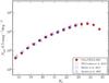 |
Fig. 6 Ks-selected galaxy number counts for UltraVISTA, in addition to some recent wide-field near-infrared surveys. The agreement with previous studies is excellent. |
3.2. Astrometric comparisons with external catalogues
We compare the positions in right ascension and declination of point sources in 2MASS with those in our UltraVISTA Ks catalogue. This is shown in Fig. 7. Note that, unlike for our photometric solutions, we do not use 2MASS as our astrometric reference catalogue but use instead a densely-sampled catalogue from the COSMOS CFHT i-band observations. The absolute astrometric calibration of COSMOS is derived from VLA 20 cm observations (Schinnerer et al. 2004), and these positions are known to be offset slightly with respect to 2MASS (Capak et al. 2007), which is indeed what we observe. Our median offsets and 1σ rms with respect to 2MASS is (0.00,0.14) arcsec and (−0.07,0.15) arcsec in RA and Dec respectively.
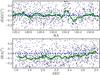 |
Fig. 7 Difference in position, in arcseconds, with respect to stars in the 2MASS, as a function of right ascension and declination (upper and lower panels respectively); every second point is plotted. The solid line shows a running median. The rms in both axes is ~0.15″. |
To verify that our astrometric reference frame is consistent with COSMOS, we carried out a similar comparison with stars in the COSMOS ACS catalogue (Leauthaud et al. 2007); this is shown in Fig. 8. In RA and Dec, no offset is observed. The 1σ rms in both directions for stars selected with 17.0 < Ks < 19.5 is ~0.08 arcsec. The internal astrometric accuracy between different UltraVISTA bands is expected to be of this order or better, i.e., much better than one 0.15″ pixel.
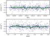 |
Fig. 8 Difference in position in arcseconds for stars between the public ACS catalogue of Leauthaud et al. (2007) and the UltraVISTA Ks stack; every second point is plotted. The solid line shows a running median. For both axes the median residuals are |

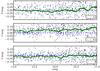 |
Fig. 9 Difference between total J,H, and Ks magnitudes of stars in UltraVISTA with sources in 2MASS. The green line corresponds to a running median. |
3.3. Photometric comparisons with external catalogues
We compare the total magnitudes of stars in our catalogue (mag_auto) with those in the 2MASS all-sky point source catalogue (Skrutskie et al. 2006). (Note also that 2MASS is used for the photometric calibration of the survey by CASU.) Of course, a significant limitation of this comparison is that the magnitude range over which sources in UltraVISTA and 2MASS overlap is relatively small. Nevertheless, the result of this test is shown in Fig. 9 where we plot UltraVISTA-2MASS magnitudes for all non-saturated stellar sources and for a total photometric error in (2MASS and UltraVISTA, summed in quadrature) of less than 0.2 mag. The thick solid line shows a running median which is always within 0.05 mag of zero for 15.0 < mag < 17.0. There is a slight systematic offset visible in H (~0.03) magnitudes; this could be due to incorrectly rescaling our exposures to slightly non-photometric images or a real offset between the two different photometric systems.
This section presents photometric comparisons between UltraVISTA and COSMOS JHKs measurements. A large amount of near-infrared observations have already been accumulated on the UltraVISTA field by the COSMOS team. These consist of Ks- (McCracken et al. 2010) and H-band observations made with WIRCam on the CFHT and J-band observations made with WFCAM on UKIRT. In all cases, these observations are shallower than the first-year UltraVISTA data set presented here. Since our stacks have the same pixel scale and tangent point as the public COSMOS data, to make our comparisons we can simply run sextractor in “dual-image” mode, choosing as detection image the UltraVISTA Ks image and as measurement images the publicly-available COSMOS Ks, H and J stacks. This approach ensures that no source matching errors are introduced. The results of this comparison is shown in Fig. 10. For test sources we choose BzK-selected stars, as described in the following section.
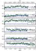 |
Fig. 10 Difference in J,H and Ks total magnitudes between BzK-selected stars with 17 < Ks < 19 in UltraVISTA and COSMOS as a function of right ascension (top three panels) and declination (bottom three panels). For clarity, only every fourth point is plotted. The thick green line corresponds to a sliding median calculated from a window of 100 points. In all cases, the differences with the COSMOS photometry is less than 0.1 mag. |
In Figs. 10 there is an offset of ~0.1–0.05 mag between UltraVISTA and the publicly-available COSMOS HKs data. We note that at brighter magnitudes, UltraVISTA magnitudes are in good agreement with 2MASS, at least for Ks and J, bands, and for H the offset reported with respect to 2MASS is smaller than the offset with respect to COSMOS magnitudes. There is also some evidence in the Ks data of a position-dependent offset. Without a third, equally deep data set, it is hard to know with certainty the origin of these offsets (especially as the VISTA and COSMOS data photometric systems are not identical). Furthermore, examining the magnitude of the offsets with respect to the COSMOS and UltraVISTA weight-maps they do not seem to be correlated with position on the focal planes of either instrument (which might be the case if there was a problem with the photometric calibration on a chip-by-chip basis). A definitive resolution to this issue awaits more involved tests, such as photometric redshift comparisons with spectroscopic data, which will be the subject of a future article.
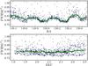 |
Fig. 11 Seeing FWHM for stars (corresponding to SEXtractor’s FWHM_WORLD parameter) selected in the BzK diagram, as a function of RA and Dec, in the Ks stack (every fourth point is plotted). As before, the solid green line corresponds to a running median. The seeing variations are small, of order ~0.05″, and vary principally as a function of RA. |
3.4. Seeing variation across the mosaics
As described above, the final UltraVISTA stack is comprised of six separate “pawprints”. At each pawprint the telescope jitter displacement is less than the separation between the detectors, so no detectors overlap. In general, each OB typically contains only images jittered around a single pawprint position, and consequently the observing conditions, in particular the average seeing is not always identical pawprint-to-pawprint. In first-year data presented here, OBs had a mix of maximum seeing constraint between 0.8″ and 1.0″; furthermore there is no minimum seeing cut. A consequence of this is that when the observations are separated paw-by-paw, in some filters, there is a variation of around 5–10% in average seeing over all 16 detectors from paw-to-paw. In the final stack, which is the combination of all pawprints, this is visible as bands of regions of slightly different seeing.
In a future UltraVISTA release we will make available stacks for which we have carried out a paw-level homogenisation (in which each of the six pawprints are convolved by a Gaussian to bring them to a common FWHM). For the moment, we report here that this effect is important for the Ks and H-band stacks. In Fig. 11 we show the seeing, calculated from SExtractor’s FWHM_WORLD parameter (which is derived from the isophotal area of the object at half maximum, and so may not be comparable to the figures listed in Table 2), as a function of right ascension and declination. Because of a sequence of pawprints with significantly better seeing, there is around a 5% variation in seeing as a function of right ascension.
3.5. Colour–magnitude and colour–colour diagrams
The large number of sources in our catalogues combined with our excellent seeing and high signal-to-noise means that we can investigate in detail the distribution of objects in colour–colour space. In Fig. 12 we plot the (J − Ks) vs. Ks distribution of sources in our Ks selected catalogue. The stellar locus is clearly visible as a narrow ridge of constant (J − Ks) colour (which one can confirm by overplotting on this diagram the location of stars identified in the ACS catalogue).
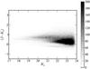 |
Fig. 12 Two-dimensional histogram showing (J − Ks) corrected aperture colour as a function of Ks total magnitude; the grey level at each bin in magnitude-colour space corresponds to the surface density of objects. The narrow ridge clearly visible at (J − Ks) ~ −0.2 corresponds to the location of stellar sources. |
Next, we consider the distribution of objects in optical and near-infrared colour–colour space, turning first to the “BzK” diagram as this allows us to cleanly separate stars and galaxies. We use the publicly-available COSMOS B and z Subaru images (Capak et al. 2007) and transform the B and z magnitudes in each catalogue following the recipes in McCracken et al. (2010) to bring our system to the “BzK” system defined in Daddi et al. (2004).
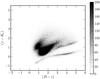 |
Fig. 13 Two-dimensional histogram of (B − z) vs. (z − Ks) corrected aperture colour for UltraVISTA. All sources detected to a 5σ limit in Ks auto magnitudes are shown. The stellar locus is clearly visible as a ridge at blue (z − Ks) colour. |
The result is shown in Fig. 13 as a two-dimensional grey-scale histogram; in this diagram and all subsequent diagrams we show all objects detected to 5σ in Ks band aperture magnitude. Several interesting features are clearly visible in this diagram: firstly the stellar locus, which is apparent as the long “ridge” feature which is relatively blue in (z − Ks); secondly, almost parallel to the stellar locus but redder in (B − z) is a second “ridge” which is comprised mainly of lower-redshift passive galaxies (Lane et al. 2007; Bielby et al. 2012). Thirdly, the division between lower-redshift normal and star-forming galaxies (the “sBzK” galaxies of Daddi et al. 2004) is clear.
In Fig. 14 we show a magnified view of the stellar locus in the BzK diagram, and we show both bright and faint stars. The position of the stellar locus does not depend on the magnitude limit, which demonstrates that there are no magnitude-dependent effects present in our data which could arise if there were issues related to an incorrect sky-subtraction.
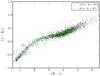 |
Fig. 14 Stellar locus for bright and faint stars in UltraVISTA (shown as points and dots respectively) in the (B − z) vs. (z − K) corrected aperture colour–colour plane. Bright and faint stars occupy the same location in colour–colour space. |
We also consider the distribution of galaxies in the purely near-infrared colour–colour space (H − Ks) vs. (Y − J), shown in Fig. 15. Again, stars and galaxies are cleanly separated.
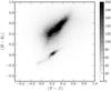 |
Fig. 15 Two-dimensional corrected aperture colour–colour (H − Ks) vs. (Y − J) histogram for all sources with total magnitude 16.0 < Ks < 23. Stars and galaxies are cleanly separated. The stellar locus corresponds to the “bump” visible at 0.2,0.1 in (Y − J) vs. (H − Ks). |
4. Summary and conclusions
In this paper we have described the first public UltraVISTA data release. This data set comprises five high-quality image stacks representing a unique combination of depth and areal coverage at near-infrared wavelengths. Our stacked images reach 5σ depths in aperture of 2″ diameter of ~25 in Y and ~24 in JHKs bands. Furthermore, it is worth noting that these depths are in agreement with the expected sensitivity of the telescope at the time of writing the original UltraVISTA survey proposal. To these limits, our Ks catalogue contains 216 268 sources. The 1σ astrometric rms in right ascension and declination for stars selected with 17.0 < Ks < 19.5 is ~0.08 arcsec in comparison to the publicly-available COSMOS ACS catalogues. Each of the stacks has sub-arcsecond seeing and the FWHM variation over the images is less than 5% in most bands. Our number counts and photometric calibration are in good agreement with previous studies.
The images and catalogues described here are publicly available from the ESOarchive10 .
At the present time of writing (April 2012), a further 250 h of UltraVISTA observations have been completed. We intend to deliver regular releases of UltraVista data products as the observations proceed towards the total 1800 h of observation time allocated to the project.
Some of these bad PSFs were caused in part by software errors in early versions of ESO’s Survey Area Definition tool: all season 1 OBs had pointing centres such that when a jitter jump went too far in one direction, the guide star fell outside the guide CCD; guiding was not active for the remaining images of that OB. This was fixed in season two observations by moving the pawprint centers. These tracking errors produce double-lobed PSFs in some images; each of the individual PSFs are smaller than the requirement and so pass our cut.
Acknowledgments
H. J. McCracken acknowledges the use of TERAPIX computing facilities. This research has made use of the VizieR catalogue access tool provided by the CDS, Strasbourg, France. This research was supported by ANR grant “ANR-07-BLAN-0228”. J.P.U.F. and B.M.J. acknowledge support from the ERC-StG grant EGGS-278202. The Dark Cosmology Centre is funded by the Danish National Research Foundation. OLF, CSJ, LT acknowledge support from the ERC advanced grant ERC-2010-AdG-268107. J.H. acknowledges support from NWO. J.S.D. acknowledges the support of the Royal Society via a Wolfson Research Merit award, and also the support of the European Research Council via the award of an Advanced Grant. The UltraVISTA team would like to thank ESO staff for scheduling and making the UltraVISTA observations, and the Cambridge Astronomy Survey Unit for providing us with pre-preprocessed UltraVISTA images. E. Bertin is thanked for useful discussions concerning the data reductions presented here.
References
- Almaini, O., Foucaud, S., Lane, K., et al. 2007, Cosmic Frontiers, ASP Conf. Ser., 379, 163 [NASA ADS] [Google Scholar]
- Arnouts, S., Walcher, C. J., Le Fèvre, O., et al. 2007, A&A, 476, 137 [NASA ADS] [CrossRef] [EDP Sciences] [Google Scholar]
- Bertin, E. 2006, Astronomical Data Analysis Software and Systems XV, ASP Conf. Ser., 351, 112 [NASA ADS] [Google Scholar]
- Bertin, E., & Arnouts, S. 1996, ApJS, 117, 393 [Google Scholar]
- Bertin, E., Mellier, Y., Radovich, M., et al. 2002, Astronomical Data Analysis Software and Systems XI, 281, 228 [NASA ADS] [Google Scholar]
- Bielby, R., Hudelot, P., McCracken, H. J., et al. 2012, A&A, in press, DOI: 10.1051/0004-6361/201118547 [Google Scholar]
- Bouwens, R. J., Thompson, R. I., Illingworth, G. D., et al. 2004, ApJ, 616, L79 [NASA ADS] [CrossRef] [Google Scholar]
- Bouwens, R. J., Illingworth, G. D., Oesch, P. A., et al. 2010, ApJ, 709, L133 [NASA ADS] [CrossRef] [Google Scholar]
- Bowler, R. A. A., Dunlop, J. S., McLure, R. J., et al. 2012, MNRAS, submitted [arXiv:1205.4270] [Google Scholar]
- Bunker, A. J., Wilkins, S., Ellis, R. S., et al. 2010, MNRAS, 409, 855 [NASA ADS] [CrossRef] [Google Scholar]
- Capak, P., Aussel, H., Ajiki, M., et al. 2007, ApJS, 172, 99 [NASA ADS] [CrossRef] [Google Scholar]
- Caputi, K. I., Cirasuolo, M., Dunlop, J. S., et al. 2011, MNRAS, 413, 162 [NASA ADS] [CrossRef] [Google Scholar]
- Casali, M., Adamson, A., Alves de Oliveira, C., et al. 2007, A&A, 467, 777 [NASA ADS] [CrossRef] [EDP Sciences] [Google Scholar]
- Cimatti, A., Daddi, E., Mignoli, M., et al. 2002, A&A, 381, L68 [NASA ADS] [CrossRef] [EDP Sciences] [Google Scholar]
- Cirasuolo, M., McLure, R. J., Dunlop, J. S., et al. 2010, MNRAS, 401, 1166 [NASA ADS] [CrossRef] [Google Scholar]
- Cowie, L. L., Gardner, J. P., Lilly, S. J., & McLean, I. 1990, ApJ, 360, L1 [NASA ADS] [CrossRef] [Google Scholar]
- Daddi, E., Cimatti, A., Renzini, A., et al. 2004, ApJ, 617, 746 [NASA ADS] [CrossRef] [Google Scholar]
- Dalton, G. B. 2006, in Ground-based and Airborne Instrumentation for Astronomy (SPIE), 1207 [Google Scholar]
- Dey, A., Cimatti, A., van Breugel, W., Antonucci, R., & Spinrad, H. 1996, ApJ, 465, 157 [NASA ADS] [CrossRef] [Google Scholar]
- Drory, N., Salvato, M., Gabasch, A., et al. 2005, ApJ, 619, L131 [NASA ADS] [CrossRef] [Google Scholar]
- Dunlop, J., Peacock, J., Spinrad, H., et al. 1996, Nature, 381, 581 [NASA ADS] [CrossRef] [Google Scholar]
- Emerson, J. P., & Sutherland, W. J. 2010, in Proc. SPIE, 7733, 773306 [Google Scholar]
- Finkelstein, S. L., Papovich, C., Giavalisco, M., et al. 2010, ApJ, 719, 1250 [Google Scholar]
- Franx, M., Labbé, I., Rudnick, G., et al. 2003, ApJ, 587, L79 [NASA ADS] [CrossRef] [Google Scholar]
- Glazebrook, K., Peacock, J. A., Miller, L., & Collins, C. A. 1991, Adv. Space Res., 11, 337 [NASA ADS] [CrossRef] [Google Scholar]
- Grogin, N. A., Kocevski, D. D., Faber, S. M., et al. 2011, ApJS, 197, 35 [NASA ADS] [CrossRef] [Google Scholar]
- Hopkins, A. M., & Beacom, J. F. 2006, ApJ, 651, 142 [NASA ADS] [CrossRef] [MathSciNet] [Google Scholar]
- Hughes, D. H., Serjeant, S., Dunlop, J., et al. 1998, Nature, 394, 241 [NASA ADS] [CrossRef] [Google Scholar]
- Ilbert, O., Capak, P., Salvato, M., et al. 2009, ApJ, 690, 1236 [NASA ADS] [CrossRef] [Google Scholar]
- Ilbert, O., Salvato, M., Floc’h, E. L., et al. 2010, ApJ, 709, 644 [NASA ADS] [CrossRef] [Google Scholar]
- Irwin, M. J., Lewis, J., Hodgkin, S., et al. 2004, in Proc. SPIE, 5493, 411 [Google Scholar]
- Koekemoer, A. M., Aussel, H., Calzetti, D., et al. 2007, ApJS, 172, 196 [NASA ADS] [CrossRef] [Google Scholar]
- Koekemoer, A. M., Faber, S. M., Ferguson, H. C., et al. 2011, ApJS, 197, 36 [NASA ADS] [CrossRef] [Google Scholar]
- Labbé, I., Franx, M., Rudnick, G., et al. 2003, AJ, 125, 1107 [NASA ADS] [CrossRef] [Google Scholar]
- Lane, K. P., Almaini, O., Foucaud, S., et al. 2007, MNRAS, 379, L25 [NASA ADS] [CrossRef] [Google Scholar]
- Lawrence, A., Warren, S. J., Almaini, O., et al. 2007, MNRAS, 379, 1599 [NASA ADS] [CrossRef] [MathSciNet] [Google Scholar]
- Leauthaud, A., Massey, R., Kneib, J.-P., et al. 2007, ApJS, 172, 219 [NASA ADS] [CrossRef] [Google Scholar]
- Lilly, S. J., & Longair, M. S. 1984, MNRAS, 211, 833 [NASA ADS] [CrossRef] [Google Scholar]
- Madau, P., Ferguson, H. C., Dickinson, M. E., et al. 1996, MNRAS, 283, 1388 [NASA ADS] [CrossRef] [Google Scholar]
- Marmo, C., & Bertin, E. 2008, Astronomical Data Analysis Software and Systems, ASP Conf. Ser., 394, 619 [Google Scholar]
- McCracken, H. J., Capak, P., Salvato, M., et al. 2010, ApJ, 708, 202 [NASA ADS] [CrossRef] [Google Scholar]
- McLean, I. S., Chuter, T. C., McCaughrean, M. J., & Rayner, J. T. 1986, Proc. SPIE, 627, 430 [NASA ADS] [CrossRef] [Google Scholar]
- McLure, R. J., Cirasuolo, M., Dunlop, J. S., Foucaud, S., & Almaini, O. 2009, MNRAS, 395, 2196 [NASA ADS] [CrossRef] [Google Scholar]
- McLure, R. J., Dunlop, J. S., Cirasuolo, M., et al. 2010, MNRAS, 403, 960 [NASA ADS] [CrossRef] [Google Scholar]
- Moffat, A. F. J. 1969, A&A, 3, 455 [NASA ADS] [Google Scholar]
- Mortlock, D. J., Warren, S. J., Venemans, B. P., et al. 2011, Nature, 474, 616 [NASA ADS] [CrossRef] [PubMed] [Google Scholar]
- Oesch, P. A., Bouwens, R. J., Illingworth, G. D., et al. 2009, ApJ, 709, L16 [Google Scholar]
- Oke, J. B. 1974, ApJS, 27, 21 [NASA ADS] [CrossRef] [Google Scholar]
- Probst, R. G. 2004, in Ground-based Instrumentation for Astronomy (SPIE), 1716 [Google Scholar]
- Puget, P., Stadler, E., Doyon, R., et al. 2004, Proc. SPIE, 5492, 978 [Google Scholar]
- Quadri, R., Marchesini, D., van Dokkum, P., et al. 2007, AJ, 134, 1103 [NASA ADS] [CrossRef] [Google Scholar]
- Schinnerer, E., Carilli, C. L., Scoville, N. Z., et al. 2004, AJ, 128, 1974 [NASA ADS] [CrossRef] [Google Scholar]
- Scott, S. E., Fox, M. J., Dunlop, J. S., et al. 2002, MNRAS, 331, 817 [NASA ADS] [CrossRef] [Google Scholar]
- Scoville, N., Abraham, R. G., Aussel, H., et al. 2007, ApJS, 172, 38 [NASA ADS] [CrossRef] [Google Scholar]
- Skrutskie, M. F., Cutri, R. M., Stiening, R., et al. 2006, AJ, 131, 1163 [NASA ADS] [CrossRef] [Google Scholar]
- Steidel, C. C., Giavalisco, M., Pettini, M., Dickinson, M., & Adelberger, K. L. 1996, ApJ, 462, L17 [NASA ADS] [CrossRef] [Google Scholar]
- Thompson, R. I., Illingworth, G., Bouwens, R., et al. 2005, AJ, 130, 1 [NASA ADS] [CrossRef] [Google Scholar]
- van Dokkum, P. G., Labbé, I., Marchesini, D., et al. 2009, PASP, 121, 2 [NASA ADS] [CrossRef] [Google Scholar]
All Tables
All Figures
|
Fig. 1 Schematic layout of UltraVISTA observations, showing deep and ultra-deep regions (hatched and filled regions respectively). The data described in this paper correspond to a uniform coverage in YJHKs of the contiguous region and to NB118 observations of the ultra-deep stripes. |
| In the text | |
|
Fig. 2 Seeing (left) and ellipticity (right) distributions for all UltraVISTA images considered. The arrow represents the median of each distribution for images classified as A or AB. Note that the distributions for each quality class have been re-normalised, and the vertical axis has been rescaled. A, AB, C represent the quality classifications described in the text. |
| In the text | |
|
Fig. 3 Full Ks mosaic, displayed using a logarithmic stretch. The background level is extremely flat, and is not perturbed near almost all bright stars. Several clusters are visible, corresponding to the many rich structures which are present in the COSMOS field. |
| In the text | |
|
Fig. 4 RGB image composed of Ks, J and Y data respectively. The size of this image represents less than 1/500th of the total area of the field. Sources as faint as Ks ~ 22 are easily visible. |
| In the text | |
|
Fig. 5 Weight-map for the first-year Ks-band data. The intensity at each pixel has been converted to an approximate 5σ limiting magnitude for an aperture of 2″ diameter. The strips at the top and bottom of the image have half the average exposure time per pixel. |
| In the text | |
|
Fig. 6 Ks-selected galaxy number counts for UltraVISTA, in addition to some recent wide-field near-infrared surveys. The agreement with previous studies is excellent. |
| In the text | |
|
Fig. 7 Difference in position, in arcseconds, with respect to stars in the 2MASS, as a function of right ascension and declination (upper and lower panels respectively); every second point is plotted. The solid line shows a running median. The rms in both axes is ~0.15″. |
| In the text | |
|
Fig. 8 Difference in position in arcseconds for stars between the public ACS catalogue of Leauthaud et al. (2007) and the UltraVISTA Ks stack; every second point is plotted. The solid line shows a running median. For both axes the median residuals are |
| In the text | |
|
Fig. 9 Difference between total J,H, and Ks magnitudes of stars in UltraVISTA with sources in 2MASS. The green line corresponds to a running median. |
| In the text | |
|
Fig. 10 Difference in J,H and Ks total magnitudes between BzK-selected stars with 17 < Ks < 19 in UltraVISTA and COSMOS as a function of right ascension (top three panels) and declination (bottom three panels). For clarity, only every fourth point is plotted. The thick green line corresponds to a sliding median calculated from a window of 100 points. In all cases, the differences with the COSMOS photometry is less than 0.1 mag. |
| In the text | |
|
Fig. 11 Seeing FWHM for stars (corresponding to SEXtractor’s FWHM_WORLD parameter) selected in the BzK diagram, as a function of RA and Dec, in the Ks stack (every fourth point is plotted). As before, the solid green line corresponds to a running median. The seeing variations are small, of order ~0.05″, and vary principally as a function of RA. |
| In the text | |
|
Fig. 12 Two-dimensional histogram showing (J − Ks) corrected aperture colour as a function of Ks total magnitude; the grey level at each bin in magnitude-colour space corresponds to the surface density of objects. The narrow ridge clearly visible at (J − Ks) ~ −0.2 corresponds to the location of stellar sources. |
| In the text | |
|
Fig. 13 Two-dimensional histogram of (B − z) vs. (z − Ks) corrected aperture colour for UltraVISTA. All sources detected to a 5σ limit in Ks auto magnitudes are shown. The stellar locus is clearly visible as a ridge at blue (z − Ks) colour. |
| In the text | |
|
Fig. 14 Stellar locus for bright and faint stars in UltraVISTA (shown as points and dots respectively) in the (B − z) vs. (z − K) corrected aperture colour–colour plane. Bright and faint stars occupy the same location in colour–colour space. |
| In the text | |
|
Fig. 15 Two-dimensional corrected aperture colour–colour (H − Ks) vs. (Y − J) histogram for all sources with total magnitude 16.0 < Ks < 23. Stars and galaxies are cleanly separated. The stellar locus corresponds to the “bump” visible at 0.2,0.1 in (Y − J) vs. (H − Ks). |
| In the text | |
Current usage metrics show cumulative count of Article Views (full-text article views including HTML views, PDF and ePub downloads, according to the available data) and Abstracts Views on Vision4Press platform.
Data correspond to usage on the plateform after 2015. The current usage metrics is available 48-96 hours after online publication and is updated daily on week days.
Initial download of the metrics may take a while.