| Issue |
A&A
Volume 544, August 2012
|
|
|---|---|---|
| Article Number | A133 | |
| Number of page(s) | 5 | |
| Section | Planets and planetary systems | |
| DOI | https://doi.org/10.1051/0004-6361/201219485 | |
| Published online | 14 August 2012 | |
Justification of the two-bulge method in the theory of bodily tides
US Naval Observatory, Washington, DC 20392, USA
e-mail: This email address is being protected from spambots. You need JavaScript enabled to view it.
Received: 25 April 2012
Accepted: 10 July 2012
Abstract
Aims. Mathematical modeling of bodily tides can be carried out in various ways. Most straightforward is the method of complex amplitudes, which is often used in the planetary science. Another method, employed both in planetary science and in astrophysics, is based on decomposition of each harmonic of the tide into two bulges oriented orthogonally to one another. We prove that the two methods are equivalent. Specifically, we demonstrate that the two-bulge method is not a separate approximation, but ensues directly from the Fourier expansion of a linear tidal theory equipped with an arbitrary rheological model involving a departure from elasticity.
Methods. To this end, we use the most general mathematical formalism applicable to linear bodily tides. To express the tidal amendment to the potential of the perturbed primary, we act on the tide-raising potential of the perturbing secondary with a convolution operator.
Results. This enables us to interconnect a complex Fourier component of the tidally generated potential of the perturbed primary with the appropriate complex Fourier component of the tide-raising potential of the secondary. Then we demonstrate how this interrelation entails the two-bulge description.
Conclusions. While less economical mathematically, the two-bulge approach has a good illustrative power, and may be employed on a par with a more concise method of complex amplitudes. At the same time, there exist situations where the two-bulge method becomes more practical for technical calculations.
Key words: binaries: close / planetary systems / stars: rotation / celestial mechanics / planets and satellites: general / planets and satellites: dynamical evolution and stability
© ESO, 2012
1. Introduction and aim
On several occasions, it was suggested by different authors to model bodily tides with superposition of two symmetrical bulges. One bulge is always aimed at the secondary, and thus implements the instantaneous reaction of the primary’s shape and potential to the tide-rising gravitational pull exerted by the secondary. This portion of the tide is called “adiabatic tide” (Zahn 1966a,b) or “elastic tide” (Ferraz Mello 2012; Krasinsky 2006). The second bulge is assumed to align orthogonally to the direction to the tide-raising secondary, and thus is set to implement the entire nonelastic portion of the primary’s deformation. This, second bulge is called “dissipative tide” (Zahn 1966a,b; Krasinsky 2006) or “creep tide” (Ferraz Mello 2012).
In this note, we demonstrate that the two-bulge method is not a separate approximation, but ensues directly from the Fourier expansion of a linear tidal theory equipped with an arbitrary rheological model involving a departure from elasticity.
2. The static linear theory of bodily tides
Let a spherical primary of radius R be subject to the gravitational pull by a secondary of mass Msec, residing at the position r∗ = (r∗, φ∗, λ∗), where r∗ ≥ R. At a surface point R = (R,φ,λ) of the primary body, the tidal potential generated by the secondary can be expanded over the Legendre polynomials Pl(cosγ) as 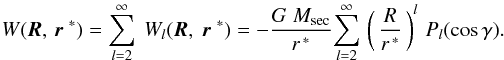 (1)Here G denotes Newton’s gravity constant, while γ is the angular separation between the vectors r∗ and R pointing from the primary’s centre. The longitudes λ, λ∗ are measured from a fixed meridian on the primary body, the latitudes φ, φ∗ being reckoned from the equator. The index l is conventionally named as the degree. In (1) the l = 0 term is missing, because it corresponds to the principal, Newtonian part of the secondary’s potential, and is not a part of the perturbation. Omission of the l = 1 term is a more subtle point related to the fact that we are describing the motion of the secondary relative to the primary body, and not in an inertial frame (see Eqs. (8)–(11) in Efroimsky & Williams 2009).
Within the linear theory, the l th term Wl(R, r∗) of the secondary’s potential generates a linear alteration of the primary’s shape. This alteration, in its turn, causes a linear amendment Ul(r) to the gravitational potential of the primary, where linear means: linear in Wl(R, r∗). The theory of potential requires that outside the primary body Ul(r) should scale with the distance as r − (l + 1). Hence the said change in the primary’s potential may be written down as 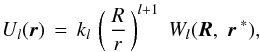 (2)where R is the mean equatorial radius of the primary, R = (R, φ, λ) is a point on the primary’s surface, while r = (r, φ, λ) is an exterior point right above the surface point R, at a radius r ≥ R. The numerical factors kl are the degree-lLove numbers calculated from the rheology of the primary body.
The overall tidally caused change of the primary’s potential thus amounts to 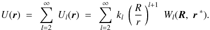 (3)
(3)
3. Dynamical linear theories of bodily tides
In realistic situations, the disturbing potential is evolving, so Eq. (1) assumes the form of 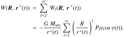 (4)Then one should expect the distortion of the primary, as well as the corresponding amendment to its potential at an exterior point r, to become a function of time: U(r, t).
3.1. Elastic dynamical tides
Had the tides contained only instantaneous, elastic components, the expressions for the tidal potential would mimic (2–3). At each instant of time t, the degree-l term of the tide-raising potential W of the orbiting secondary would generate instantaneously an appropriate degree-l term of the tidal potential of the primary: 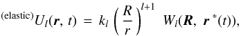 (5)so the total tidal amendment to the potential of the primary would look:
 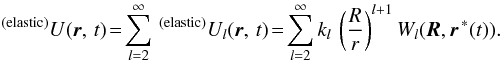 (6)Needless to say, in realistic materials the internal friction prevents the tidal deformation from being instantaneous.
3.2. Realistic dynamical tides
To describe deviation from elasticity, we spell out the two basic assumptions whereon a linear dynamical theory of bodily tides is based:
-
[1]
tidal deformation is linear with respect to the stress generatedby the tide-raising potential;
-
[2]
the deformation is not fully elastic: it incorporates both an immediate and delayed portions (delayed – relative to the tide-raising potential).
Mathematically, assumption [1] means that an infinitesimal increment ΔWl(R,r∗(t ′)), whereby the perturbing potential increased at the time t ′ in the past, results in a proportional present-time increment of the tidally distorted shape of the primary and, accordingly, in a proportional increment of the tidal amendment to its potential: 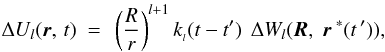 (7)kl(t − t ′) being a function describing the delayed reaction. The mathematical form of this function is defined by the rheology of the body and by its self-gravitation.
Thus the addition Ul to the primary’s potential gets expressed through the tide-raising potential Wl by a linear integral operator: 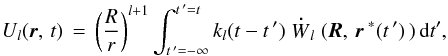 (8)overdot denoting a time derivative. Integration of (8) by parts renders:
 ![Mathematical equation: \begin{eqnarray} U_{\it l}(\erbold,\,t)&=&\left(\frac{R}{r} \right)^{{\it l}+1}\left[k_l(0)W_l(t) - k_l(\infty)W_l(-\infty)\right] \nonumber\\ &&+ \left(\frac{R}{r} \right)^{{\it l}+1}\int_{-\infty}^{t} {\bf\dot{\it{k}}}_{{_l}}(t-t\,')\, W_{\it{l}} (\eRbold, \erbold^{\;*}(t\,')\,)\,{\rm d}t, \label{8b} \end{eqnarray}](/articles/aa/full_html/2012/08/aa19485-12/aa19485-12-eq43.png) (9)where the relaxed term − kl(∞)W( − ∞) should be neglected. Indeed, the current events cannot be influenced by the perturbation Wl( − ∞) in the infinite past, wherefore kl(∞) = 0. Of the remaining two terms, the unrelaxed term kl(0)Wl(t) reflects the elastic part of the deformation, while the integral expresses the delayed components – viscous and anelastic.
(9)where the relaxed term − kl(∞)W( − ∞) should be neglected. Indeed, the current events cannot be influenced by the perturbation Wl( − ∞) in the infinite past, wherefore kl(∞) = 0. Of the remaining two terms, the unrelaxed term kl(0)Wl(t) reflects the elastic part of the deformation, while the integral expresses the delayed components – viscous and anelastic.
Assumption [2] means that both the unrelaxed term kl(0)Wl(t) and the delayed term given by the integral should be kept. As explained in Efroimsky (2012a,b), the relaxed term may be easily incorporated into the integral, where it should show up multiplied with a Heaviside step function Θ(t − t ′). Then our expression for the tidal potential will acquire the simple form of 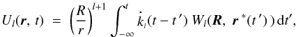 (10)kl(t − t ′) now incorporating both the delayed-reaction terms and the elastic term kl(0) Θ(t − t ′). The elastic part will then enter the kernel
  as kl(0) δ(t − t′), with δ(t − t ′) being the Dirac delta function. Integration of this term will furnish kl(0)Wl(t), as in (9).
4. Fourier components of tidal stresses and strains
4.1. Tidal modes and tidal frequencies
The sidereal angle and the spin rate of a tidally-perturbed primary are normally denoted with θ and  , while the node, pericentre, and mean anomaly of a tide-raising secondary, as seen from the primary, are denoted with Ω, ω, and ℳ.
In the Darwin-Kaula theory, the tide-raising potential W, the primary’s deformation, and the tidal amendment U to the primary’s potential are expanded over the modes 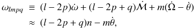 (11)l, m, p, q being integers, and n being the mean motion. Dependent upon the values of the mean motion, spin rate, and the indices, the tidal modes ωlmpq may be positive or negative or zero.
The actual forcing frequencies of the resulting stresses and strains in the primary’s material are the absolute values of the tidal modes: 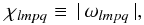 (12)so these frequencies are always positive.
4.2. Fourier expansions
In practical calculations, it is extremely convenient to employ complex stresses and strains, under the convention that the actual, physical quantities are the real parts of their complex counterparts. This way, the Fourier series for the stress and strain look: ![Mathematical equation: \begin{eqnarray} \sigma_{\gamma\nu}(t)\, &=&\sum_{s=0}^{\infty}\,\sigma_{\gamma\nu}(\chi_{s})\,\cos\left[\,\chi_{s} t+\varphi_{\sigma}(\chi_{s})\right]\; \nonumber\\ &=&\sum_{s=0}^{\infty}\, {\cal{R}}{\it{e}}\left[\,{\bar{\sigma}}_{\gamma\nu}(\chi_{s})\,\;\exp\left({\inc \chi_{s} t}\right)\right],~~~~~~~~~~ \label{12} \\ u_{\gamma\nu}(t) &=&\sum_{s=0}^{\infty}\,u_{\gamma\nu}(\chi_{s})\,\cos\left[\,\chi_{s}t+ \varphi_{u}(\chi_{s})\right] \; \nonumber\\ &=&\sum_{s=0}^{\infty}\, {\cal{R}}{\it{e}}\left[\,{\bar{u}}_{\gamma\nu}(\chi_{s})\;\,\exp\left({{{\, \inc\chi_{s} t}}}\right)\,\;\right],~~~~~~~~~~ \label{13} \end{eqnarray}](/articles/aa/full_html/2012/08/aa19485-12/aa19485-12-eq67.png) γν being tensor indices, and s being a concise notation for lmpq. The complex amplitudes are
γν being tensor indices, and s being a concise notation for lmpq. The complex amplitudes are ![Mathematical equation: \begin{eqnarray} {\bar{{\sigma}}_{\gamma\nu}}(\chi)={{{\sigma}}_{\gamma\nu}}(\chi) \exp\left[{\inc\varphi_\sigma(\chi)}\right], ~{\bar{{u}}_{\gamma\nu}}(\chi)={{{u}}_{\gamma\nu}}(\chi) \exp\left[{\inc\varphi_u(\chi)}\right], \label{compamp} \label{14} \end{eqnarray}](/articles/aa/full_html/2012/08/aa19485-12/aa19485-12-eq71.png) (15)where the initial phases ϕσ(χ) and ϕu(χ) are chosen so that the real amplitudes σγν(χs) and uγν(χs) are non-negative.
(15)where the initial phases ϕσ(χ) and ϕu(χ) are chosen so that the real amplitudes σγν(χs) and uγν(χs) are non-negative.
For a continuous spectrum, the sums get replaced with integrals over frequency: 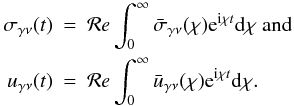 (16)Similarly, the tide-raising potential Wl and the potential Ul of the primary get expanded into a sum or integral over the tidal modes:
 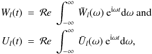 (17)where the complex amplitudes are expressed via the real amplitudes and the initial phases by
![Mathematical equation: \begin{eqnarray} &&{\bar{{W}}_{l}}(\omega)={{{W}}_{l}}(\omega) \exp\left[{\inc\varphi_{W_l}(\omega)}\right],\nonumber\\ &&{\bar{{U}}_{l}}(\omega)={{{U}}_{l}}(\omega) \exp\left[{\inc\varphi_{U_l}(\omega)}\right] . \label{17} \end{eqnarray}](/articles/aa/full_html/2012/08/aa19485-12/aa19485-12-eq79.png) (18)
(18)
The phases ϕWl(ω) and ϕUl(ω) can always be set in such a way that the real amplitudes Wl(χ) and Ul(χ) are non-negative.
Both in (16) and (17), the actual, physical spectral components are the real parts of the complex ones. However, there also is an important difference between (16) and (17). While the stresses and strains are habitually expanded in (16) over positive frequencies χ only, the potentials in (17) are expanded over the tidal modes ω, which can be positive or negative or zero, as demonstrated in the Darwin-Kaula theory of tides.
It is of course a common fact that a real function can be decomposed into a Fourier series or integral over only positive frequencies. This way, expansions of the potentials over χ ≡ | ω | may appear to be sufficient, because a contribution from some negative tidal mode ω < 0 can be shown to coincide with the contribution from the appropriate positive mode | ω | > 0. Therefore, (17) may be rewritten simply as 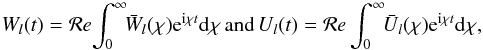 (19)where
  and
and  .
.
Surprisingly, the theory of tides is a rare exception from the rule, in that this theory does distinguish between the contribution from a negative tidal mode and that from a positive mode of the same absolute value. Fortunately, the difference shows up only at the stage when one calculates tidal forces or torques (Efroimsky 2012a,b). As in the current paper we discuss potentials only, we shall ignore this subtlety and shall employ (19) instead of (17).
4.3. Dynamical analogues to the Love number
Insertion of (19) into (10) entails 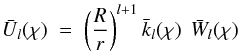 (20)or, in a more detailed form:
 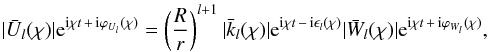 (21)where the complex function
  (22)is a Fourier component of the kernel
  of the integral operator (10). The kernels are named Love functions, a term suggested by Churkin (1998). The functions
  are called complex Love numbers, in understanding however that these “numbers” change with frequency. An approach similar to (22) was taken by Mathis & Le Poncin Lafitte (2009). These authors introduced a complex impedance as the ratio between the complex Love number and the static Love number. Their Eq. (107) is equivalent to our (22), up to a convention on the sign of the argument.
We see from (21) that at each frequency χ, the negative argument ϵl(χ) is a measure of lagging of the spectral component Ul(χ), relative to appropriate spectral component Wl(χ):  (23)
(23)
5. Decomposition of a tidal mode into an in-phase part and an in-quadrature (lagging by 90°) part
In the expression (21), we may set the initial phase of  to be zero, and reckon the phase of
  from
from  . This will enable us to single out, in , a part which is in phase with , and also to see what part of
  is out of phase with
  .
.
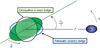 |
Fig. 1 Decomposition of the semidiurnal tide into the elastic and dissipative components. The primary is spinning at the rate |


According to (23), nullification of the phase of makes the phase of equal to the negative argument of  . So (21) will assume the form of
  (24)where we introduced simplified notations Ul 0(χ), Wl 0(χ) and kl 0 for real amplitudes:
  (25)By means of the Euler formula, (24) can be trivially expanded as
![Mathematical equation: \begin{eqnarray} && U_{l{{_{\,0}}}}(\chi)~\left[\, \cos\left(\chi t - \epsilon_l(\chi)\,\right) + i \sin\left(\chi t - \epsilon_l(\chi)\, \right) \right] = \nonumber\\ &&\left(\frac{R}{r}\right)^{2l+1}\! k_{l{{_{\,0}}}}(\chi) \left[ \cos\epsilon_l(\chi) \!-\! i \sin\epsilon_l(\chi) \right] ~W_{l{{_{\,0}}}}(\chi) \left[\, \cos(\chi t) + i \sin( \chi t)\right]. \label{24}\nonumber\\ \end{eqnarray}](/articles/aa/full_html/2012/08/aa19485-12/aa19485-12-eq121.png) (26)The actual, physical tide-raising potential Wl(χ) is the real part of the complex . So it is rendered by Wl0(χ)cos(χt), where we set the initial phase nil, as agreed above. Similarly, the actual, physical tidal potential Ul(χ) is the real part of the complex Ul(χ), and it reads as:
(26)The actual, physical tide-raising potential Wl(χ) is the real part of the complex . So it is rendered by Wl0(χ)cos(χt), where we set the initial phase nil, as agreed above. Similarly, the actual, physical tidal potential Ul(χ) is the real part of the complex Ul(χ), and it reads as: 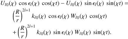 (27)In this expression for the actual real Ul, we see not one but two terms. One is the elastic part of the tide, a part that is in phase with the real Wl. This is the term proportional to cos(χt):
 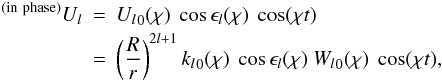 (28)We see that the “response factor” is equal to kl0(χ)cosϵl(χ), where kl0(χ) is the real amplitude of the complex Love number (call this amplitude dynamical Love number).
The second component is the in-quadrature term, which is proportional to sin(χt): 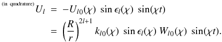 (29)Naturally, the expression of this term via Wl contains kl0(χ)sinϵl(χ).
Therefore, as soon as we express Ul via Wl by an integral operator permitting delayed reaction (Eq. (9)), we automatically arrive at the two components of the tidal Ul, at each frequency involved, – the adiabatic component and the dissipative component (using the terms of Zahn 1966) or the elastic one and the creep one (as Ferraz-Mello 2012 named them)1.
Similar decomposition will take place for the harmonic modes of the primary’s surface elevation, except that the Love number hl will be involved instead of kl. For the principal, {lmpq} = { 2200 } , tidal mode, this situation is illustrated, in a very exaggerated manner, by Fig. 1.
It should finally be mentioned that in the case of stars and giant planets it is, technically, difficult to solve the emerging hydrodynamical problem analytically. Therefore, in practical calculations of fluid equilibrium tides in such bodies, the two-bulge method is the only known elegant option of getting an acceptable analytical solution. One first solves the hydrodynamical equations governing the adiabatic component (28). The adiabatic adjustment of the structure is deduced from the hydrostatic balance. Then, since the velocity field is preserved along isobars, one obtains the radial component of the adiabatic velocity field induced by the tide. The subsequent calculation of the horizontal component is based on the velocity field being divergence-free. The knowledge of the adiabatic velocity field makes it possible to determine the viscous force. This force drives the dissipative component of the velocity field. The process leads to mass redistribution inside the body, and thus to perturbation of the density and gravitational potential (29). The described, two-bulge approach is available because in the fluid equilibrium tide the dissipative component is much weaker than the adiabatic component. The method is implemented, e.g., in the work by Remus et al. (2012a), which furthers the original two-bulge approach offered by Zahn (1966).
6. Conclusions
In this short note, we pointed out a simple rule linking the two methods (or, possibly better to say, two languages), in which bodily tides have been described by different authors. The language of complex amplitudes is more economical and is conventional to those who studied the theory of vibrations, in physics or engineering. The language of two bulges turns out to be equivalent to that of complex amplitudes. Although less economical mathematically, the two-bulges language has some illustrative power, and may be employed on a par with the more concise method of complex amplitudes. At the same time, there exist situations where the two-bulge method is more practical for technical calculations (like, e.g., in Remus et al. 2012a,b).
Importantly, the existence of two mutually orthogonal bulges at each tidal frequency is not a separate approximation (as was presumed by some of the devotees of the two-bulge method), but is a consequence of the linearity assumption implemented by the integral operator (10). As soon as we say that the tidal deformation is linear but not fully elastic – this deformation can be decomposed, at each tidal frequency, into an in-phase and an in-quadrature part.
Also see the work by Krasinsky (2006), who employed the terms elastic and dissipative.
Acknowledgments
It is my pleasure to thank Françoise Remus for her useful advices and for her help in preparing the figure. I also acknowledge with gratitude the stimulating conversations on the topic of this work, which I had on various occasions with Sylvio Ferraz Mello, Valéry Lainey, Valeri Makarov, Stephane Mathis, and Jean-Paul Zahn.
References
- Churkin, V. A. 1998, The Love Numbers for the Models of Inelastic Earth, Preprint No. 121, Institute of Applied Astronomy, St. Petersburg, Russia (in Russian) [Google Scholar]
- Efroimsky, M. 2012a, Celest. Mech. Dyn. Astron., 112, 283 [NASA ADS] [CrossRef] [Google Scholar]
- Efroimsky, M. 2012b, ApJ, 746, 150 [NASA ADS] [CrossRef] [Google Scholar]
- Efroimsky, M., & Williams, J. G. 2009, Celest. Mech. Dyn. Astron., 104, 257 [Google Scholar]
- Ferraz-Mello, S. 2012, Celest. Mech. Dyn. Astron., submitted [arXiv:1204.3957] [Google Scholar]
- Mathis, S., & Le Poncin-Lafitte, C. 2009, A&A, 497, 889 [NASA ADS] [CrossRef] [EDP Sciences] [Google Scholar]
- Krasinsky, G. A. 2006, Celest. Mech. Dyn. Astron., 96, 169 (In this paper, see formulae (96–97) and the subsequent Sects. 4.2–4.3.) [Google Scholar]
- Remus, F., Mathis, S., Zahn, J.-P. 2012a, A&A, 544, A132 [NASA ADS] [CrossRef] [EDP Sciences] [Google Scholar]
- Remus, F., Mathis, S., Zahn, J.-P., & Lainey, V. 2012b, A&A, 541, A165 [NASA ADS] [CrossRef] [EDP Sciences] [Google Scholar]
- Zahn, J.-P. 1966a, Ann. Astrophys., 29, 313 [NASA ADS] [Google Scholar]
- Zahn, J.-P. 1966b, Ann. Astrophys., 29, 489 [Google Scholar]
All Figures
|
Fig. 1 Decomposition of the semidiurnal tide into the elastic and dissipative components. The primary is spinning at the rate |
| In the text | |
Current usage metrics show cumulative count of Article Views (full-text article views including HTML views, PDF and ePub downloads, according to the available data) and Abstracts Views on Vision4Press platform.
Data correspond to usage on the plateform after 2015. The current usage metrics is available 48-96 hours after online publication and is updated daily on week days.
Initial download of the metrics may take a while.