© ESO, 2012

1. Introduction

The ESO Gaia space observatory during its early phase will adopt a peculiar scanning procedure covering the two ecliptic poles every six hours. This will provide the possibility for the initial testing and calibration of the scientific equipment, software and operations. The areas can be used also in future for monitoring the stability of photometric and spectroscopic instruments, especially in cases of contingency. For this aim, in the 1°  ×  1° fields at both ecliptic poles special catalogs of astrometric, photometric and spectral data will be compiled from ground-based observations (Voss & Bastian 2007; Altmann & Bastian 2009).

In the area of the North Ecliptic Pole (NEP) the photometric and especially spectral investigations in the optical range are scanty. The objects between R magnitudes 13 and 23 were measured and analysed in the B, R, K system by Kümmel & Wagner (2000, 2001), and between R magnitudes 16 and 25 in the Sloan Digital Sky Survey (SDSS) u, g, r, i, z system by Hwang et al. (2007). The main emphasis of these investigations, covering about 1 square degree around NEP, was the separation of galaxies from stars and the photometric classification of galaxies. Jeon et al. (2010) determined B, R and I magnitudes for the objects with R magnitudes between 12 and 23, but outside the Hwang et al. field and outside the standard Gaia field. Recently, the results of the APASS survey of the northern sky by AAVSO in the B, V and the SDSS g, r, i systems down to V = 16 mag became available¹.

In the infrared, some objects in the Gaia NEP field were observed by IRAS (Beichman et al. 1988; Hacking & Houck 1987), AKARI (Matsuhara et al. 2006; Lee et al. 2007; Takagi et al. 2012; Ko et al. 2012), WISE and Spitzer (Jarrett et al. 2011) surveys. About 15 NEP K-giants were classified and applied for the absolute calibration of the Spitzer (Reach et al. 2005), AKARI (Tanabé et al. 2008) and WISE (Jarrett et al. 2011) space telescopes. The stars down to J = 16 mag were measured in the 2MASS J, H, K_s survey (Skrutskie et al. 2006). Bower et al. (1996), Henry et al. (2001), Voges et al. (2001) and Gioia et al. (2003) in the NEP area have made identifications between the ROSAT X-ray and optical sources.

As an input to the Gaia catalog of the NEP stars, we decided to provide seven-color photometric data for stars down to V ≈ 16 mag in the Vilnius system, together with spectral and luminosity classes and interstellar extinctions determined from this multicolor photometry. We also present the transformations of the Vilnius magnitudes to the broad-band SDSS and Gaia systems.

2. Observations and reductions

The investigated area, centered at (RA, Dec, J2000) = (18:00:20, +66:33:40) and limited by the coordinates RA 17:54:04–18:06:40, Dec +65:57:00–+67:10:10, is shown in Fig. 1. CCD observations in the filters of the Vilnius seven-color photometric system were obtained in August and September of 2009 with the Maksutov-type 35/51 cm telescope of the Molėtai Observatory in Lithuania. The camera is of the VersArray 1300B type with liquid nitrogen cooling. The backside-illuminated 1340  ×  1300 pixel chip (pixel size 20  ×  20 μm) has the Unichrom UV-enhancement coating (see Zdanavičius & Zdanavičius 2003, for details). The image scale is 3.38′′ per pixel, the field size is 1.26°  ×  1.22°. To avoid the effect of some defective pixels, some of the exposures were taken with slight shifts. The filter set used was described in our earlier papers (Zdanavičius et al. 2008, 2010a). The total number of exposures is 50, see Table 1.

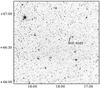Fig. 1 The observed NEP area in the V filter. The planetary nebula NGC 6543 (Cat’s Eye Nebula) is indicated.

The flatfielding and bias corrections were taken into account using the IRAF package. Instrumental magnitudes were determined combining the aperture and PSF methods. More details on the reduction procedures can be found in Zdanavičius et al. (2008). The (x,y)-coordinates of stars were transformed to right ascensions and declinations using the USNO-B1.0 catalog (Monet et al. 2003).

Since the NEP area has no standard stars in the Vilnius system, for creating a set of local standards we applied the tie-in method with the open cluster NGC 752 in Andromeda. Short tie-in exposures were obtained during nights with stable transparency and at similar zenith distances. The values of magnitudes and color indices of 26 stars in NGC 752, measured photoelectrically, were taken from Bartašiūtė et al. (2007). The same exposures of NGC 752 were used to obtain the equations for transformation of the instrumental magnitudes and color indices to the standard Vilnius system. The reliability of the transformation equations was verified and confirmed using an area in the open cluster M 29 in Cygnus containing 40 stars measured photoelectrically by Kazlauskas & Jasevičius (1986).

However, after the reduction of instrumental color indices to the standard system, some differences of zero-points can be present due to possible small non-linearities of color equations, interstellar reddening effects and the errors of atmospheric extinction corrections. To verify the correspondence of zero-points of color indices to the standard system, we applied a series of interstellar reddening-free Q₁, Q₂ diagrams. Here ${\mathit{Q}}_{\mathrm{1234}}\mathrm{=}\mathrm{(}{\mathit{m}}_{\mathrm{1}}\mathrm{-}{\mathit{m}}_{\mathrm{2}}\mathrm{)}\mathrm{-}\mathrm{(}{\mathit{E}}_{\mathrm{12}}\mathit{/}{\mathit{E}}_{\mathrm{34}}\mathrm{)}\hspace{0.17em}\mathrm{(}{\mathit{m}}_{\mathrm{3}}\mathrm{-}{\mathit{m}}_{\mathrm{4}}\mathrm{)}\mathit{,}$(1)where m are the magnitudes in four (or three) passbands, m₁ − m₂ and m₃ − m₄ are the two color indices and E₁₂ and E₃₄ are the corresponding color excesses. The intrinsic sequences in the Q₁, Q₂ diagrams for different luminosity classes were calculated from the intrinsic color indices and color-excess ratios given in the Straižys (1992) monograph. The ratios of color excesses were taken for the normal interstellar reddening law. In some of the Q₁, Q₂ diagrams small displacements of the NEP stars from the intrinsic sequences were found and excluded by correcting zero-points of the corresponding color indices.

Table 2 contains the catalog of V magnitudes and color indices of 948 stars down to V ≈ 16.2 mag in the standard Vilnius system. Among them, 293 stars have all seven magnitudes, 331 stars have no ultraviolet (U and P) magnitudes, and 324 stars have no ultraviolet and violet (X) magnitudes. The rms errors of magnitudes and color indices given in the table are  ≤ 0.03 mag. Color indices with the errors between 0.026–0.030 mag are marked with colons. The stars Nos. 1–624 were measured with sufficient accuracy in 7, 6 or 5 mag. The stars Nos. 625–948 were too faint in the ultraviolet and violet passbands, and for them only the magnitudes Y, Z, V and S were measured with sufficient accuracy. The distribution of the measured stars in magnitudes is given in Fig. 2, separately for the stars Nos. 1–624 and 625–948.

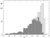Fig. 2 Star counts in the magnitude V bins. The counts for stars with ultraviolet U and P and/or violet magnitudes X (numbers 1–624 in Table 2) are shown in gray colons, the counts for stars without magnitudes U, P and X (numbers 625–948) – in white colons.

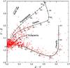Fig. 3 The Y–Z vs. Z–V diagram used for two-dimensional classification of K and M stars. Intrinsic sequences of luminosity classes V, IV, III and I and the interstellar reddening line for AV = 0.3 mag are shown. The slope of the reddening line is EY − Z/EZ − V = 1.8. The NEP stars with Z–V  >  0.2 are plotted in red.

3. Photometric classification

For the determination of spectral and luminosity classes of individual stars three different methods were used: (1) the σQ “COMPAR” method which uses matching of 14 different reddening-free Q-parameters of a program star to those of about 12 000 standard stars with known MK spectral types; (2) the “dxq” method which uses matching of color indices of a program star with those of a set of 300 standards formed from the mean intrinsic color indices for stars with different spectral types and absolute magnitudes, and different amounts of interstellar reddening, and (3) the “QQ” method which uses up to 12 different two-Q diagrams calibrated in spectral and luminosity classes. The methods are described in more details by Zdanavičius et al. (2010b).

Since the interstellar reddening in the NEP area is quite small (A_V < 0.3, E_B − V < 0.1, see the next section), for the classification of late-type stars we applied not only reddening-free Q-parameters, but also two-color diagrams with the appropriate calibration in terms of spectral classes. In Fig. 3 we show the diagram Y–Z vs. Z–V with the intrinsic sequences for V, IV, III and I luminosity classes and the stars with Z–V > 0.2 from Table 2. It is evident that K- and M-type star sequences in this diagram are well separated. Here a strong luminosity effect is due to the position of the Z passband on the Mg I triplet lines and MgH band which are very strong in dwarfs. This diagram allows to classify K–M stars in the NEP area without the ultraviolet and violet magnitudes (stars Nos. 625–948).

The results of photometric classification in spectral and luminosity classes for about 500 stars are presented in Table 2. For the remaining stars only spectral classes (without luminosities) are given. Visual binaries with distances between the components less than about 5 arcsec were either excluded from the catalog, or the given magnitudes and color indices correspond to both components together. Such close binaries were identified by an inspection of their images in the DSS2-Red survey exposed in SkyView, the Internet Virtual Telescope site. These stars are listed in notes at the end of the table. Spectral classes are written in lower-case letters to designate that they have been determined from multicolor photometry. About ten stars were suspected as metal-deficient, probably they are F–G subdwarfs and G–K metal-deficient giants. The table also contains interstellar extinctions obtained as described in next section.

4. Interstellar reddening and extinction

Interstellar reddenings for 360 stars with two-dimensional classification were calculated as differences between the observed and intrinsic color indices, ${\mathit{E}}_{\mathit{Y}\mathrm{-}\mathit{V}}\mathrm{=}\mathrm{(}\mathit{Y}\mathrm{-}\mathit{V}{\mathrm{)}}_{\mathrm{obs}}\mathrm{-}\mathrm{(}\mathit{Y}\mathrm{-}\mathit{V}{\mathrm{)}}_{\mathrm{0}}\mathit{.}$(2)The extinctions and distances of stars were calculated by the equations $\begin{array}{ccc}& & {\mathit{A}}_{\mathit{V}}\mathrm{=}\mathrm{4.16} {\mathit{E}}_{\mathit{Y}\mathrm{-}\mathit{V}}\mathit{,}\\ & & \mathrm{5}\log \hspace{0.17em}\mathit{d}\mathrm{=}\mathit{V}\mathrm{-}{\mathit{M}}_{\mathit{V}}\mathrm{+}\mathrm{5}\mathrm{-}{\mathit{A}}_{\mathit{V}}\mathit{.}\end{array}$Intrinsic color indices (Y–V)₀ and absolute magnitudes M_V for corresponding MK types were taken from Straižys (1992). For some stars the reddening (and extinction) values were found to be slightly negative, this can be explained by the observational errors and by cosmic dispersion of the intrinsic color indices. For these stars we accepted A_V = 0.

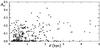Fig. 4 Dependence of the interstellar extinction AV on the distance d. Only the stars with the most reliable two-dimensional classification, with the ultraviolet and violet magnitudes available, are plotted.

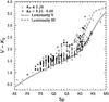Fig. 5 Dependence of V − Ks on spectral class for two ranges of interstellar extinction AV for stars with the most reliable two-dimensional classification. The intrinsic sequences for luminosity classes V and III are determined as described in the text.

The extinctions A_V are listed in Table 2 and plotted against distance in Fig. 4. As is expected for the Galactic latitude of NEP, no dependence of A_V on distance is seen. Only a few stars exhibit the extinctions larger than 0.3 mag. The average value of A_V for stars with d > 500 pc (i.e. outside the Galactic dust layer) is 0.10 ± 0.01 mag, with the standard deviation 0.14 mag. Calculating this average, some small negative extinctions were included. This value is in satisfactory agreement with the average value A_V = 0.13 mag from Schlegel et al. (1998), based on the IRAS and COBE/DIRBE dust emission surveys at 100 μm with the new calibration by Schlafly et al. (2010) and Schlafly & Finkbeiner (2011) at low reddenings. The dispersion of the extinction values, which is observed in Fig. 4, partly can be real being caused by a cloudy structure of the Galactic interstellar dust layer. Many stars with A_V = 0 at distances d > 500 pc are seen through windows between the clouds.

A partly independent estimate of interstellar extinction in the area can be obtained by combining the Vilnius V magnitudes with the K_s magnitudes of the 2MASS system. Figure 5 shows a plot of the V − K_s colors of 554 stars against our spectral classes. The stars are devided in two groups according to their values of A_V from Table 2: (1) with A_V ≤ 0.20 mag (dots) and (2) with A_V between 0.21 and 0.40 mag (crosses). The intrinsic colors (V − K_s)₀ for luminosity V and III stars are determined summing the (V − H)₀ values for the Johnson system from Straižys (1992) and the H − K_s values from Straižys & Lazauskaitė (2009). It is evident that the stars of group (2) exhibit larger deviations upward from the intrinsic sequences for their luminosity classes. The largest deviation is about 0.45 mag, what corresponds to E_B − V = 0.16 or A_V = 0.52 mag. Taking into account observational errors, classification errors and the errors of intrinsic color indices, this value of A_V is close to maximum values of A_V obtained in the Vilnius system. However, we do not exclude possibility that in some cases the reddening can originate not from interstellar dust but from a secondary cool component in a binary system.

5. Transformation to the SDSS system

As it was mentioned in the Introduction, the NEP area contains the magnitudes of stars and galaxies in the SDSS (or shortly “Sloan”) system u, g, r, i, z published by Hwang et al. (2007). Almost all stars in their catalog are fainter than V = 16, while our catalog contains brighter stars, with V magnitudes between 12 and 16. Thus, our results could be used to extend the SDSS catalog to brighter magnitudes if the appropriate transformation equations were available. To our knowledge, no attempts of such transformation have been done in the past.

The differences between the SDSS and Vilnius magnitudes were calculated by synthetic photometry convolving the spectral energy distributions of stars, the response functions of the passbands and the interstellar extinction law: 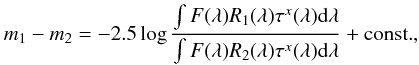${\mathit{m}}_{\mathrm{1}}\mathrm{-}{\mathit{m}}_{\mathrm{2}}\mathrm{=}\mathrm{-}\mathrm{2.5}\log \frac{\mathrm{\int }\mathit{F}\mathrm{\left(}\mathit{\lambda }\mathrm{\right)}{\mathit{R}}_{\mathrm{1}}\mathrm{\left(}\mathit{\lambda }\mathrm{\right)}{\mathit{\tau }}^{\mathit{x}}\mathrm{\left(}\mathit{\lambda }\mathrm{\right)}\mathrm{d}\mathit{\lambda }}{\mathrm{\int }\mathit{F}\mathrm{\left(}\mathit{\lambda }\mathrm{\right)}{\mathit{R}}_{\mathrm{2}}\mathrm{\left(}\mathit{\lambda }\mathrm{\right)}{\mathit{\tau }}^{\mathit{x}}\mathrm{\left(}\mathit{\lambda }\mathrm{\right)}\mathrm{d}\mathit{\lambda }}\mathrm{+}\mathrm{const}\mathit{.}\mathit{,}$(5)where m₁ and m₂ are magnitudes defined by the response functions R₁(λ) and R₂(λ), F(λ) is the energy flux distribution function in the spectrum of a star, τ^x(λ) is the transmittance function of interstellar dust for x unit masses. The response functions of the Vilnius system were taken from Straižys (1992) and of the SDSS system from Doi et al. (2010, Fig. 8). Spectral energy distributions (SEDs) of 50 stars of different spectral and luminosity classes are from Straižys & Sviderskienė (1972). In the ultraviolet (300–360 nm), these SEDs were corrected taking into account the data from the OAO-2, TD-1 and IUE space missions (Straižys 1996). To investigate the effect of interstellar reddening, synthetic magnitude differences were also calculated up to A_V = 4.8 mag accepting the normal interstellar reddening law from Straižys (1992, Table 3). The normalizing values of magnitude differences were calculated accepting F(ν) = const. (the AB magnitude scale) for the SDSS magnitudes and F(λ) of unreddened O8-type star for the Vilnius magnitudes.

Figures 6–8 show the differences between the SDSS magnitudes u, g and r and the magnitude V of the Vilnius system, plotted against the temperature-sensitive color index Y–V.² The first magnitude in the differences, plotted on the y axis, in all cases has a shorter mean wavelength than the second, this makes the differences positive. In the figures dots are main-sequence stars, crosses are giants and circles are supergiants. The interstellar reddening lines (in some cases they are considerably curved) are shown for the three spectral types – O8 V, A0 V and K5 III up to A_V = 4.8 mag. It is evident that in the whole temperature range the magnitude transformations are nonlinear and luminosity- and reddening-dependent. This means that the transformation equations must contain not only the Y–V color index, sensitive to the temperature, but also other indices which could take into account nonlinearities and luminosity differences. The largest deviations are observed for M-type stars with Y–V > 0.9 for M-dwarfs and  > 1.1 for M-giants, see Fig. 6, which also show the largest luminosity effects. The transformation of magnitudes of reddened stars (shifted along the reddening lines) is very complicated too, especially in the case of the ultraviolet magnitudes.

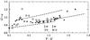Fig. 6 Difference of the magnitude U of the Vilnius system and the magnitude u of the SDSS system as a function of the temperature-sensitive color Y–V. Luminosity class V stars are dots, class III – crosses and class I – circles. The reddening lines for the three spectral types, O8 V, A0 V and K5 III, are shown. The same designations are used in Figs. 7, 8 and 11–13.

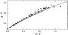Fig. 7 Difference of the magnitude g of the SDSS system and the magnitude V of the Vilnius system as a function of Y–V.

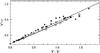Fig. 8 Difference of the magnitude V of the Vilnius system and the magnitude r of the SDSS system as a function of Y–V.

For obtaining the transformation equations from the Vilnius to the SDSS system we used 116 stars in the open cluster M 67 measured in both systems. The SDSS data were taken from the SDSS Photometric Catalog, Release 7 (Abazajian et al. 2009), and the Vilnius data are from Laugalys et al. (2004). The M 67 stars brighter than V = 14 mag with saturated images in the SDSS catalog were excluded. These stars are easily seen in different two-color diagrams showing large deviations from the sequences of fainter stars.

As it was shown in Figs. 6–8, due to nonlinearity of medium-band and broad-band relations, and luminosity and interstellar reddening effects, there is no simple equation correlating the Vilnius and SDSS magnitudes which would depend only on the star temperature-sensitive color. Therefore we applied equations with the terms containing two and even three color indices of the Vilnius system. The aim of combining these terms was to achieve the minimum residuals of the observed differences m–V of individual stars from those given by the transformation equations. The equations are valid only for unreddened stars or for small reddenings (as in M 67 and NEP). They are also not applicable for M-type stars.

The following transformation equations were obtained: $\begin{array}{ccc}\mathit{u}& \mathrm{=}& \mathit{V}\mathrm{-}\mathrm{0.435}\mathrm{+}\mathrm{0.113}\hspace{0.17em}\mathrm{(}\mathit{U}\mathrm{-}\mathit{V}\mathrm{)}\mathrm{+}\mathrm{0.845}\hspace{0.17em}\mathrm{(}\mathit{P}\mathrm{-}\mathit{V}\mathrm{)}\mathit{,}\\ \mathit{g}& \mathrm{=}& \mathit{V}\mathrm{-}\mathrm{0.294}\mathrm{+}\mathrm{0.047}\mathrm{(}\mathit{X}\mathrm{-}\mathit{V}\mathrm{)}\mathrm{+}\mathrm{0.632}\mathrm{(}\mathit{Y}\mathrm{-}\mathit{V}\mathrm{)}\mathrm{+}\mathrm{0.461}\mathrm{(}\mathit{Z}\mathrm{-}\mathit{V}\mathrm{)}\mathit{,}\end{array}$or $\mathit{g}\mathrm{=}\mathit{V}\mathrm{-}\mathrm{0.216}\mathrm{+}\mathrm{0.648}\hspace{0.17em}\mathrm{(}\mathit{Y}\mathrm{-}\mathit{V}\mathrm{)}\mathrm{+}\mathrm{0.553}\hspace{0.17em}\mathrm{(}\mathit{Z}\mathrm{-}\mathit{V}\mathrm{)}\mathit{,}$(8)when X–V is absent; $\mathit{r}\mathrm{=}\mathit{V}\mathrm{+}\mathrm{0.118}\mathrm{-}\mathrm{0.444}\hspace{0.17em}\mathrm{(}\mathit{Z}\mathrm{-}\mathit{V}\mathrm{)}\mathrm{-}\mathrm{0.407}\hspace{0.17em}\mathrm{(}\mathit{V}\mathrm{-}\mathit{S}\mathrm{)}$(9)to transform from the ZVS system or $\mathit{r}\mathrm{=}\mathit{V}\mathrm{+}\mathrm{0.112}\mathrm{-}\mathrm{0.429}\hspace{0.17em}\mathrm{(}\mathit{Y}\mathrm{-}\mathit{V}\mathrm{)}\mathrm{-}\mathrm{0.400}\hspace{0.17em}\mathrm{(}\mathit{Z}\mathrm{-}\mathit{V}\mathrm{)}$(10)to transform from the YZV system.

Zero-points in the equations include the normalization differences of both systems: color indices in the Vilnius system are normalized to zero for unreddened O8 V stars while the SDSS system is normalized to the isoenergetic source for unit frequency intervals (the AB system). The residuals of the magnitudes u, g and r (differences between the observed and the calculated by the equations) are shown in Fig. 9. They mean that the rms errors of the transformed magnitudes are  ± 0.03 mag for u and  ± 0.02 mag for g and r.

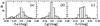Fig. 9 Residuals of the SDSS magnitudes of 116 stars of the open cluster M 67 transformed from the Vilnius system by Eqs. (6)–(10).

The transformed magnitudes in the Sloan system are listed in Table 3 which is constructed in a similar way as Table 2: for the stars with numbers 1–624 all seven Vilnius magnitudes or at least five of them (without U and P) are available, while for the fainter stars with numbers 625–948 only four magnitudes, Y, Z, V and S have been used. For these stars the SDSS u magnitude could not be obtained.

It is difficult to estimate the external accuracy of our transformations since the observational data in the original SDSS system for the stars brighter than V = 16 mag in the NEP area are absent. Therefore in Fig. 10 (panels (b) and (c)) we compare the SDSS g and r magnitudes transformed from the Vilnius system with the magnitudes in the same passbands transformed from the Tycho B_T and V_T system by Pickles & Depagne (2010). In panel (a) of the same figure a comparison of the V magnitudes of the Vilnius system and the V_T magnitudes of the Tycho system (both V magnitudes are observed) is given. The agreement between the g and r magnitudes transformed from the two systems down to V = 11.5 mag is satisfactory, with σ of the order of  ± 0.03. However, for fainter stars the differences increase drastically as a result of the decreasing precision of the observed Tycho magnitudes, see panel (a).

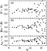Fig. 10 Panel a) gives differences of the observed V magnitudes for 52 NEP stars common in the Vilnius and Tycho systems. Panels b) and c) for the same stars give differences of the SDSS magnitudes g and r transformed from both systems.

6. Transformation to the Gaia system

The ESO Gaia space observatory, to be launched in 2013, will provide photometry in a few passbands: the panchromatic (superbroad) magnitude G covering the spectral range from about 350 nm to 1000 nm, two broad-band G_BP and G_RP magnitudes in the ranges 330–680 nm and 640–1000 nm and one narrow-band G_RVS magnitude in the region of the Paschen limit and the Ca II triplet, 847–874 nm. These Gaia photometric passbands and the corresponding magnitudes were analyzed by Jordi et al. (2010) using a method of synthetic photometry. They also calculated the relationships between colors involving Gaia magnitudes and colors in other broad-band systems (U, B, V, R, I of Johnson-Cousins, u, g, r, i, z of SDSS and H_p, B_T,V_T of Hipparcos-Tycho). In the present paper, we investigate the relationships between the magnitudes of the Vilnius and Gaia photometric systems.

The applied method is the same as that used to calculate the synthetic relations between the Vilnius and SDSS magnitudes. The response functions of the Gaia magnitudes were taken from Jordi et al. (2010). The expected variations in the form of the BP and RP response functions in the Gaia focal plane (Jordi 2012) are not taken into account. The zero-point was defined considering that all Gaia magnitudes coincide with the V magnitude of the Vilnius system for an unreddened star of spectral type A0 V. One must bear in mind that all color indices in the Vilnius system are equal to zero for an unreddened star of spectral type O8 V.

The Gaia magnitudes G, G_BP and G_RP were transformed from the magnitude V of the Vilnius system. The magnitude G_RVS was not considered since it is completely outside the range covered by the Vilnius passbands. In Figs. 11–13 differences of the Gaia magnitudes and the Vilnius magnitude V are plotted against Y–V. The relations show nonlinearities and different location of luminosity sequences and interstellar reddening lines.

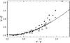Fig. 11 Difference of the magnitude V of the Vilnius system and the magnitude G of the Gaia system as a function of Y–V.

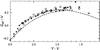Fig. 12 Difference of the magnitude GBP of the Gaia system and the magnitude V of the Vilnius system as a function of Y–V.

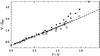Fig. 13 Difference of the magnitude V of the Vilnius system and the magnitude GRP of the Gaia system as a function of Y–V.

In order to increase the transformation accuracy to Gaia magnitudes, a few color indices of the Vilnius system have been used. In the case of G_BP, two transformation equations with different coefficients are used in different color ranges.

For obtaining the Gaia G and G_BP magnitudes, the following transformation equations were used: $\mathit{G}\mathrm{=}\mathit{V}\mathrm{-}\mathrm{0.035}\mathrm{+}\mathrm{0.078}\mathrm{(}\mathit{Y}\mathrm{-}\mathit{V}\mathrm{)}\mathrm{+}\mathrm{0.141}\mathrm{(}\mathit{Z}\mathrm{-}\mathit{V}\mathrm{)}\mathrm{-}\mathrm{0.620}\mathrm{(}\mathit{V}\mathrm{-}\mathit{S}{\mathrm{)}}^{\mathrm{2}}\mathit{,}$(11)when V–S  <  1.04 (i.e. without M-type stars), ${\mathit{G}}_{\mathrm{BP}}\mathrm{=}\mathit{V}\mathrm{-}\mathrm{0.207}\mathrm{+}\mathrm{0.479}\mathrm{(}\mathit{X}\mathrm{-}\mathit{V}\mathrm{)}\mathrm{-}\mathrm{0.084}\mathrm{(}\mathit{V}\mathrm{-}\mathit{S}\mathrm{)}\mathrm{-}\mathrm{0.126}\mathrm{(}\mathit{X}\mathrm{-}\mathit{V}{\mathrm{)}}^{\mathrm{2}}$(12)for stars with X–V  ≤  1.8 (earlier than K1 V and G5 III) and ${\mathit{G}}_{\mathrm{BP}}\mathrm{=}\mathit{V}\mathrm{-}\mathrm{0.234}\mathrm{+}\mathrm{1.550}\mathrm{(}\mathit{Y}\mathrm{-}\mathit{V}\mathrm{)}\mathrm{-}\mathrm{0.498}\mathrm{(}\mathit{V}\mathrm{-}\mathit{S}\mathrm{)}\mathrm{-}\mathrm{0.626}\mathrm{(}\mathit{Y}\mathrm{-}\mathit{V}{\mathrm{)}}^{\mathrm{2}}$(13)for stars with X–V  >  1.8 and  <  2.7, where M-type stars begin.

The residuals from Eqs. (11–13) are about  ± 0.03 mag. Since in the range of the G_RP passband only one Vilnius passband, S on the Hα line, is present, the transformations are less accurate – the equation ${\mathit{G}}_{\mathrm{RP}}\mathrm{=}\mathit{V}\mathrm{+}\mathrm{0.256}\mathrm{-}\mathrm{0.094}\mathrm{(}\mathit{Y}\mathrm{-}\mathit{V}\mathrm{)}\mathrm{-}\mathrm{1.603}\mathrm{(}\mathit{V}\mathrm{-}\mathit{S}\mathrm{)}\mathrm{+}\mathrm{0.160}\mathrm{(}\mathit{V}\mathrm{-}\mathit{S}{\mathrm{)}}^{\mathrm{2}}$(14)gives the residuals up to  ± 0.06 mag.

In the case when interstellar reddening is present, all the coefficients in the above equations become slightly dependent on color excesses. We do not give these dependences since the majority of NEP stars are either unreddened or their color excesses are quite small (E_B − V ≤ 0.1).

For the stars without U, P and X magnitudes available (Table 2, serial numbers 625–948) the Gaia magnitudes were obtained by the following equations: $\begin{array}{ccc}& & \mathit{G}\mathrm{=}\mathit{V}\mathrm{-}\mathrm{0.034}\mathrm{+}\mathrm{0.311}\mathrm{(}\mathit{Y}\mathrm{-}\mathit{V}\mathrm{)}\mathrm{-}\mathrm{0.252}\mathrm{(}\mathit{Z}\mathrm{-}\mathit{V}\mathrm{)}\\ & & \mathrm{-}\mathrm{0.746}\mathrm{(}\mathit{Y}\mathrm{-}\mathit{V}{\mathrm{)}}^{\mathrm{2}}\mathit{,}\\ & & {\mathit{G}}_{\mathrm{BP}}\mathrm{=}\mathit{V}\mathrm{-}\mathrm{0.236}\mathrm{+}\mathrm{1.062}\mathrm{(}\mathit{Y}\mathrm{-}\mathit{V}\mathrm{)}\mathrm{+}\mathrm{0.338}\mathrm{(}\mathit{Z}\mathrm{-}\mathit{V}\mathrm{)}\\ & & \mathrm{-}\mathrm{0.874}\mathrm{(}\mathit{Y}\mathrm{-}\mathit{V}{\mathrm{)}}^{\mathrm{2}}\mathit{,}\\ & & {\mathit{G}}_{\mathrm{RP}}\mathrm{=}\mathit{V}\mathrm{+}\mathrm{0.313}\mathrm{-}\mathrm{1.338}\mathrm{(}\mathit{Y}\mathrm{-}\mathit{V}\mathrm{)}\mathrm{-}\mathrm{1.019}\mathrm{(}\mathit{Z}\mathrm{-}\mathit{V}\mathrm{)}\\ & & \mathrm{+}\mathrm{0.148}\mathrm{(}\mathit{Y}\mathrm{-}\mathit{V}{\mathrm{)}}^{\mathrm{2}}\end{array}$for A-F-G stars (Y–V  <  0.65), and $\begin{array}{ccc}& & \mathit{G}\mathrm{=}\mathit{V}\mathrm{-}\mathrm{1.433}\mathrm{+}\mathrm{3.651}\mathrm{(}\mathit{Y}\mathrm{-}\mathit{V}\mathrm{)}\mathrm{-}\mathrm{0.826}\mathrm{(}\mathit{Z}\mathrm{-}\mathit{V}\mathrm{)}\\ & & \mathrm{-}\mathrm{2.261}\mathrm{(}\mathit{Y}\mathrm{-}\mathit{V}{\mathrm{)}}^{\mathrm{2}}\mathit{,}\\ & & {\mathit{G}}_{\mathrm{BP}}\mathrm{=}\mathit{V}\mathrm{-}\mathrm{0.152}\mathrm{+}\mathrm{0.728}\mathrm{(}\mathit{Y}\mathrm{-}\mathit{V}\mathrm{)}\mathrm{-}\mathrm{0.043}\mathrm{(}\mathit{Z}\mathrm{-}\mathit{V}\mathrm{)}\\ & & \mathrm{-}\mathrm{0.291}\mathrm{(}\mathit{Y}\mathrm{-}\mathit{V}{\mathrm{)}}^{\mathrm{2}}\mathit{,}\\ & & {\mathit{G}}_{\mathrm{RP}}\mathrm{=}\mathit{V}\mathrm{-}\mathrm{1.853}\mathrm{+}\mathrm{3.983}\mathrm{(}\mathit{Y}\mathrm{-}\mathit{V}\mathrm{)}\mathrm{-}\mathrm{1.375}\mathrm{(}\mathit{Z}\mathrm{-}\mathit{V}\mathrm{)}\\ & & \mathrm{-}\mathrm{2.729}\mathrm{(}\mathit{Y}\mathrm{-}\mathit{V}{\mathrm{)}}^{\mathrm{2}}\end{array}$for K-type stars (0.65 < Y–V < 1.0).

The transformed magnitudes are given in Table 3. For 13 M-type stars the Gaia magnitudes are absent.

7. Conclusions

We have presented the results of photometry of 948 stars down to V = 16.2 mag in the Vilnius seven-color system at the North Ecliptic Pole, which is an important addition to the catalogs of astrometric, photometric and spectral data for the initial testing and calibration of the scientific equipment, software and operations onboard the Gaia space observatory (Voss & Bastian 2007; Altmann & Bastian 2009). The seven-color photometry allowed us to classify about 500 stars in spectral and luminosity classes and to determine their interstellar reddenings and extinctions. For the remaining stars one-dimensional spectral classes are given. A few stars are suspected to be metal-deficient F–G subdwarfs and G–K giants. These results will be important in verifying the classification accuracy from the Gaia BP, RP and RVS spectra for stars of different brightness. The mean interstellar extinction value in the area, A_V = 0.10 mag, is found to be close to that estimated by the Schlegel et al. (1998) dust map constructed from observations of dust emission at 100 μm, with the revised calibration.

For convenience, we also present the transformations of the Vilnius magnitudes to the SDSS and Gaia systems. For this task we have derived the relations between the Vilnius and SDSS magnitudes using observational data in the open cluster M 67 and synthetic photometry. The relations between the Vilnius and Gaia systems were determined only by synthetic photometry. These relations are interesting examples of the transformation between the medium-band, broad-band and superbroad-band photometric systems. The accuracy of the transformed magnitudes can be characterized by the residuals from the equations which for different magnitudes range from  ± 0.03 to 0.06 mag. The catalogs of photometric and spectral data of Tables 2 and 3 are available at the CDS.

Acknowledgments

The use of the MegaPipe, SkyView and Simbad databases is acknowledged. We are thankful to M. S. Bessell for the useful referee comments and Edmundas Meištas for his help in preparing the paper.

References

All Tables

All Figures

	Fig. 1 The observed NEP area in the V filter. The planetary nebula NGC 6543 (Cat’s Eye Nebula) is indicated.
In the text

	Fig. 2 Star counts in the magnitude V bins. The counts for stars with ultraviolet U and P and/or violet magnitudes X (numbers 1–624 in Table 2) are shown in gray colons, the counts for stars without magnitudes U, P and X (numbers 625–948) – in white colons.
In the text

	Fig. 3 The Y–Z vs. Z–V diagram used for two-dimensional classification of K and M stars. Intrinsic sequences of luminosity classes V, IV, III and I and the interstellar reddening line for AV = 0.3 mag are shown. The slope of the reddening line is EY − Z/EZ − V = 1.8. The NEP stars with Z–V  >  0.2 are plotted in red.
In the text

	Fig. 4 Dependence of the interstellar extinction AV on the distance d. Only the stars with the most reliable two-dimensional classification, with the ultraviolet and violet magnitudes available, are plotted.
In the text

	Fig. 5 Dependence of V − Ks on spectral class for two ranges of interstellar extinction AV for stars with the most reliable two-dimensional classification. The intrinsic sequences for luminosity classes V and III are determined as described in the text.
In the text

	Fig. 6 Difference of the magnitude U of the Vilnius system and the magnitude u of the SDSS system as a function of the temperature-sensitive color Y–V. Luminosity class V stars are dots, class III – crosses and class I – circles. The reddening lines for the three spectral types, O8 V, A0 V and K5 III, are shown. The same designations are used in Figs. 7, 8 and 11–13.
In the text

	Fig. 7 Difference of the magnitude g of the SDSS system and the magnitude V of the Vilnius system as a function of Y–V.
In the text

	Fig. 8 Difference of the magnitude V of the Vilnius system and the magnitude r of the SDSS system as a function of Y–V.
In the text

	Fig. 9 Residuals of the SDSS magnitudes of 116 stars of the open cluster M 67 transformed from the Vilnius system by Eqs. (6)–(10).
In the text

	Fig. 10 Panel a) gives differences of the observed V magnitudes for 52 NEP stars common in the Vilnius and Tycho systems. Panels b) and c) for the same stars give differences of the SDSS magnitudes g and r transformed from both systems.
In the text

	Fig. 11 Difference of the magnitude V of the Vilnius system and the magnitude G of the Gaia system as a function of Y–V.
In the text

	Fig. 12 Difference of the magnitude GBP of the Gaia system and the magnitude V of the Vilnius system as a function of Y–V.
In the text

	Fig. 13 Difference of the magnitude V of the Vilnius system and the magnitude GRP of the Gaia system as a function of Y–V.
In the text

References

- Abazajian, K. N., Adelman-McCarthy, J. K., Agueros, M. A., et al. 2009, ApJS, 182, 543, = CDS Vizier Catalog II/294 [NASA ADS] [CrossRef] [Google Scholar]
- Altmann, M., & Bastian, U. 2009, Ecliptic Poles Catalogue, version 1.1, Tech. Rep. GAIA-C3-TN-ARI-MA-002-01 [Google Scholar]
- Bartašiūtė, S., Deveikis, V., Straižys, V., & Bogdanovičius, A. 2007, Baltic Astron., 16, 199 [NASA ADS] [Google Scholar]
- Beichman, C. A., Neugebauer, G., Habing, H. J., Clegg, P. E., & Chester, T. J. 1988, Infrared astronomical satellite (IRAS) catalogs and atlases, Vol. 1: Explanatory supplement (Washington DC: GPO), http://irsa.ipac.caltech.edu/applications/Gator/ [Google Scholar]
- Bower, R. G., Hasinger, G., Castander, F. J., et al. 1996, MNRAS, 281, 59 [NASA ADS] [CrossRef] [Google Scholar]
- Doi, M., Tanaka, M., Fukugita, M., et al. 2010, AJ, 139, 1628 [NASA ADS] [CrossRef] [Google Scholar]
- Gioia, I. M., Henry, J. P., Mullis, C. R., et al. 2003, ApJS, 149, 29 [NASA ADS] [CrossRef] [Google Scholar]
- Hacking, P., & Houck, J. R. 1987, ApJS, 63, 311 [NASA ADS] [CrossRef] [Google Scholar]
- Henry, J. P., Gioia, I. M., Mullis, C. R., et al. 2001, ApJ, 553, L109 [NASA ADS] [CrossRef] [Google Scholar]
- Hwang, N., Lee, M. G., Lee, H. M., et al. 2007, ApJS, 172, 583 [NASA ADS] [CrossRef] [Google Scholar]
- Jarrett, T. H., Cohen, M., Masci, F., et al. 2011, ApJ, 735, 112 [NASA ADS] [CrossRef] [Google Scholar]
- Jeon, Y., Im, M., Ibrahimov, M., et al. 2010, ApJS, 190, 166 [NASA ADS] [CrossRef] [Google Scholar]
- Jordi, C. 2012, BP/RP Bandwidth Non-Uniformity, Tech. Rep. GAIA-C5-TN-UB-CJ-048-001 [Google Scholar]
- Jordi, C., Gebran, M., Carrasco, J. M., et al. 2010, A&A, 523, A48 [NASA ADS] [CrossRef] [EDP Sciences] [Google Scholar]
- Kazlauskas, A., & Jasevičius, V. 1986, Bull. Vilnius Obs., 75, 18 [Google Scholar]
- Ko, J., Im, M., Lee, H. M., et al. 2012, ApJ, 745, 181 [NASA ADS] [CrossRef] [Google Scholar]
- Kümmel, M. W., & Wagner, S. J. 2000, A&A, 353, 867 [NASA ADS] [Google Scholar]
- Kümmel, M. W., & Wagner, S. J. 2001, A&A, 370, 384 [NASA ADS] [CrossRef] [EDP Sciences] [Google Scholar]
- Laugalys, V., Kazlauskas, A., Boyle, R. P., et al. 2004, Baltic Astron., 13, 1 [NASA ADS] [Google Scholar]
- Lee, H. M., Im, M., Wada, T., et al. 2007, PASJ, 59, 529 [Google Scholar]
- Matsuhara, H., Wada, T., Matsuura, S., et al. 2006, PASJ, 58, 673 [NASA ADS] [Google Scholar]
- Monet, D. G., Levine, S. E., Canzian, B., et al. 2003, AJ, 125, 984 [NASA ADS] [CrossRef] [Google Scholar]
- Pickles, A., & Depagne, E. 2010, PASP, 122, 1437 [NASA ADS] [CrossRef] [Google Scholar]
- Reach, W. T., Megeath, S. T., Cohen, M., et al. 2005, PASP, 117, 978 [NASA ADS] [CrossRef] [Google Scholar]
- Schlafly, E. F., & Finkbeiner, D. P. 2011, ApJ, 737, 103 [NASA ADS] [CrossRef] [Google Scholar]
- Schlafly, E. F., Finkbeiner, D. P., Schlegel, D. J., et al. 2010, ApJ, 725, 1175 [NASA ADS] [CrossRef] [Google Scholar]
- Schlegel, D. J., Finkbeiner, D. P., & Davis, M. 1998, ApJ, 500, 525, http://irsa.ipac.caltech.edu/applications/DUST [NASA ADS] [CrossRef] [Google Scholar]
- Skrutskie, M. F., Cutri, R. M., Stiening, R., et al. 2006, AJ, 131, 1163 [NASA ADS] [CrossRef] [Google Scholar]
- Straižys, V. 1992, Multicolor Stellar Photometry (Tucson, Arizona: Pachart Publishing House), http://www.itpa.lt/MulticolorStellarPhotometry/ [Google Scholar]
- Straižys, V. 1996, unpublished [Google Scholar]
- Straižys, V., & Lazauskaitė, R. 2009, Baltic Astron., 18, 19 [Google Scholar]
- Straižys, V., & Sviderskienė, Z. 1972, Bull. Vilnius Obs., 35, 3 [NASA ADS] [Google Scholar]
- Takagi, T., Matsuhara, H., Goto, T., et al. 2012, A&A, 537, A24 [NASA ADS] [CrossRef] [EDP Sciences] [Google Scholar]
- Tanabé, T., Sakon, I., Cohen, M., et al. 2008, PASJ, 60, 375 [NASA ADS] [CrossRef] [Google Scholar]
- Voges, W., Henry, J. P., Briel, U. G., et al. 2001, ApJ, 553, L119 [NASA ADS] [CrossRef] [Google Scholar]
- Voss, B., & Bastian, U. 2007, Ecliptic Poles Scanning Law and the Ecliptic Poles Catalogue, Tech. Rep. GAIA-C3-SP-ARI-BV-001-01 [Google Scholar]
- Zacharias, N., Finch, C., Girard, T., et al. 2010, AJ, 139, 2184, UCAC3 Catalogue, CDS I/315 [NASA ADS] [CrossRef] [Google Scholar]
- Zdanavičius, J., & Zdanavičius, K. 2003, Baltic Astron., 12, 642 [NASA ADS] [Google Scholar]
- Zdanavičius, J., Bartašiūtė, S., Boyle, R. P., Vrba, F. J., & Zdanavičius, K. 2010a, Baltic Astron., 19, 63 [NASA ADS] [Google Scholar]
- Zdanavičius, J., Bartašiūtė, S., & Zdanavičius, K. 2010b, Baltic Astron., 19, 35 [NASA ADS] [Google Scholar]
- Zdanavičius, K., Zdanavičius, J., Straižys, V., & Kotovas, A. 2008, Baltic Astron., 17, 161 [NASA ADS] [Google Scholar]