| Issue |
A&A
Volume 544, August 2012
|
|
|---|---|---|
| Article Number | A58 | |
| Number of page(s) | 7 | |
| Section | Interstellar and circumstellar matter | |
| DOI | https://doi.org/10.1051/0004-6361/201219130 | |
| Published online | 26 July 2012 | |
Dust shell model of the water fountain source IRAS 16342–3814
1 School of Physics and Astronomy, EC Stoner Building, University of Leeds, Leeds LS2 9JT, UK
e-mail: This email address is being protected from spambots. You need JavaScript enabled to view it.
2 Okayama Astrophysical Observatory, 3037-5 Honjo, Kamogata, Asakuchi, 719-0232 Okayama, Japan
Received: 28 February 2012
Accepted: 28 June 2012
Abstract
Aims. We investigate the circumstellar dust shell of the water fountain source IRAS 16342–3814.
Methods. We performed two-dimensional radiative transfer modeling of the dust shell, taking into account previously observed spectral energy distributions (SEDs) and our new J-band imaging and H- and KS-band imaging polarimetry obtained using the VLT/NACO instrument.
Results. Previous observations expect an optically thick torus in the equatorial plane because of a striking bipolar appearance and a large viewing angle of 30−40°. However, models with such a torus as well as a bipolar lobe and an AGB shell cannot fit the SED and the images simultaneously. We find that an additional optically and geometrically thick disk located inside a massive torus solves this problem. The masses of the disk and the torus are estimated to be 0.01 M⊙ at the amax = 100 μm dust and 1 M⊙ at amax = 10 μm dust, respectively.
Conclusions. We discuss a possible formation scenario for the disk and torus based on a similar mechanism to the equatorial back flow. IRAS 16342–3814 is expected to undergo mass loss at a high rate. The radiation from the central star is shielded by the dust that was ejected in the subsequent mass loss event. As a result, the radiation pressure on dust particles cannot govern the motion of the particles anymore. The mass loss flow can be concentrated in the equatorial plane by help of an interaction, which might be the gravitational attraction by the companion, if it exists in IRAS 16342–3814. A fraction of the ejecta is captured in a circum-companion or circum-binary disk and the remains are escaping from the central star(s) and form the massive torus.
Key words: stars: AGB and post-AGB / circumstellar matter / radiative transfer / stars: individual: IRAS 16342-3814
© ESO, 2012
1. Introduction
IRAS 16342 − 3814 (hereafter I16342), also known as OH 344.1+5.8, is an oxygen-rich proto(pre)-planetary nebula (PPN) exhibiting a striking pair of bipolar lobes. He et al. (2008) detected a low 12CO/13CO intensity ratio of 1.7 and concluded that 12C is being converted into 13C via the hot bottom burning process, suggesting that the initial mass of the central star is as high as ≳ 5 M⊙. Another characteristic of this object is high-velocity maser components. The velocities of OH masers at 1612, 1665, and 1667 MHz are ~65 km s-1, which are much faster than those in many OH/IR stars (Likkel & Morris 1988). The H2O masers are even faster ~130−180 km s-1 (Zuckerman & Lo 1987; Likkel & Morris 1988). The apparent dynamical ages of the masers are very short at ≲ 100 yr (Claussen et al. 2009; Imai et al. 2012). The H2O masers are more like jets in appearance than the typical AGB winds. Because of these maser properties, objects like I16342 are called “water fountain source (WFS)” (Likkel & Morris 1988; Imai et al. 2007). So far, 14 objects are classified into this group (Imai et al. 2007; Suárez et al. 2009; Walsh et al. 2009; Gómez et al. 2011). Many PNs exhibit jets, which cannot be explained with only the generalised interacting stellar wind (GISW) model (Sahai & Trauger 1998). The WFSs are thought to be progenitors that provide crucial clues to understanding the shaping mechanisms of these PNs.
Because of the peculiar maser properties in WFS, many works have studied H2O and OH masers. In I16342, the best-studied object, the circumstellar dust shell (CDS) has been studied. The optical and near-infrared (NIR) images show a distinct bipolar appearance with an extension of ~5″ lying at a position angle of 73° (Sahai et al. 1999). In the optical, the eastern lobe is fainter by a factor of ~0.1 with respect to the western one. Sahai et al. (1999) estimated the viewing angle to be ~40° from the 1612 MHz OH maser distribution, i.e. the western polar axis is tilted by ~40° toward the observer. The Keck II L′-band images show a corkscrew-like feature in the bipolar lobes (Sahai et al. 2005). Although a clear correlation with the distribution of the H2O maser jets is not found, the feature is probably a kind of precessing jet that carved out the inner part of the bipolar lobe. In the mid-infrared (MIR), an elliptic flux structure was detected (Meixner et al. 1999; Dijkstra et al. 2003). However, the high-resolution VISIR/VLT data resolved a pair of bipolar lobes with a separation of the flux peaks of 0 92 at 11.85 μm (Verhoelst et al. 2009; Lagadec et al. 2011). These results suggest an optically and geometrically thick torus in the equatorial plane of this object.
In this present work, we have modeled the dust shell of I16342 by means of two-dimensional radiative transfer calculations. The spectral energy distribution (SED) collected from various sources and our new NIR polarimetric data obtained using the VLT/NACO instrument were used to constrain the physical parameters of the CDS. In Sects. 2 and 3, our VLT/NACO observations and radiative transfer calculations are presented. In Sect. 4, we discuss the structure and the formation of the inner most region of the dust shell.
2. VLT/NACO imaging polarimetry
2.1. Observations and data reduction
We obtained standard (non-polarimetric) images in the J-band and polarimetric images in the H and KS band using the CONICA camera with the NAOS adaptive optics (AO) system mounted on the Very Large Telescope (VLT). The S27 camera with a pixel scale of 27.15 mas pix-1 was operated in the Double_RdRstRd read-out mode. For the wavefront sensing, the N20C80 dichroic filter was used. Because the target is extended in the optical and near-infrared and the central star feature is invisible, a single star 2MASS J16374030–3820087 (mK = 8.0 mag) at a 97 separation from the target was monitored for the AO reference.
The J-band imaging was carried out on August 4, 2009. The natural seeing was 05 − 06 according to the ESO observatories ambient conditions data base. The exposure time was 30 s. per frame and six images were taken at each four jitter positions, yielding a total integration time of 12 min. The raw data were reduced by subtracting the dark frame, dividing by the flat frame, and combining the all science data. We used the photometric data of GSPC S875-C (mJ = 11.085 mag) for the flux calibration, which was offered in the ESO standard calibration plan. The signal-to-noise ratios per beam is 40 − 240 in regions with the surface brightnesses of 2 × 10-15 W m-2 μm-1 arcsec-2 or brighter.
The H and KS band imaging polarimetry was carried out on 2 May, 2009. The natural seeing varied between 10 and 15 during the observations. The turnable half-waveplate (HWP) and the Wollaston prism with a slit width of 3″ were used to measure linear polarization. The slit position is aligned along the long axis of the target at a position angle of 73°. Four image sets were taken at position angles of the HWP of 0°, 45°, 22.5°, and 67.5°. Seven and ten jitter positions were performed and exposure times were 60 s. and 30 s. per frame, in the H and KS band, respectively. The total integration times were 28 min. in the H band and 20 min. in the KS band. After the subtraction of the dark frames, the sky background levels and flat fielding, the Stokes IQU parameter images were obtained by combining the ordinary and extra-ordinary ray frames. The data of a single star HD 147283 were used for polarization calibration (PH = 0.91 ± 0.05% and PK = 0.48 ± 0.04%; Whittet et al. 1992). Our uncalibrated measurements are PH = 3.6% and PK = 1.7%. These discrepancies include the instrumental polarization and some other error sources. In observations that require a polarization accuracy better than 1%, such as the line spectropolarimetry, a careful calibration is essential (see Witzel et al. 2011). On the other hand, an ~ 2% accuracy is acceptable in most cases of optical and infrared imaging polarimetry of bipolar reflection nebulae. The difference of these tolerances also results from the different interests of the observations. In imaging polarimetry, the spatial information is important, but is affected by the photon noise and the temporal variations in the shape of the point-spread function (PSF) because of the use of small “aperture” sizes, e.g. beam sizes. It is opposite in the aperture polarimetry or line spectropolarimetry. We assumed that the discrepancies between our observations and the previous aperture polarimetry (Whittet et al. 1992) are caused by the instrumental polarization and the offset Stokes Q/I and U/I values. The estimated signal-to-noise ratios per beam of the Stokes I images in regions with surface brightness of 2 × 10-15 W m-2 μm-1 arcsec-2 or brighter are 60 − 120 in the H band and 20−120 in the KS band. The errors of linear polarization are PH ~ 3% and PK ~ 2%.
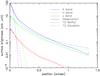 |
Fig. 1 Radial plot of the PSFs in the J (red), H (green), and KS (blue) bands. The surface brightnesses are normalized. The observations are compared with the two one-dimensional PSF models of Moffat and Gaussian functions. |
Parameters of the PSF model.
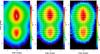 |
Fig. 2 J, H, and KS band images of IRAS 16342–3814 obtained using NACO on the VLT. The polarization vector lines are overlaid on the H and KS band images. The field of view is |

We evaluated the shapes and sizes of the beam. In the J band, a single star detected in the science frame was examined. In the H and KS band the standard star was used because no single stars are detected in the science frames. We found that most of flux from the reference stars is detected within  from the central star, and the star feature is nearly circular. Therefore, the star feature was tangentially averaged and was examined as a one-dimensional PSF. Figure 1 shows the radial plot of the PSFs in the J, H and KS bands. The solid curves are for the observations. The measured full width at half maximum (FWHM) are
  ,
,  , and
, and  in the J, H and KS bands, respectively. The real PSF sizes of the object would be somewhat larger than them because an offset AO referencing was applied. We examined a Gaussian model (e.g., Bendinelli et al. 1990) and a Moffat model (Moffat 1969). The model PSF forms are given by
 ![Mathematical equation: \hbox{$F_\mathrm{Gauss}\left(r\right)=A\exp[-1/2\left(r/\sigma\right)^2]$}](/articles/aa/full_html/2012/08/aa19130-12/aa19130-12-eq47.png) and
and ![Mathematical equation: \hbox{$F_\mathrm{Moffat}\left(r\right)=A/[1+\left(r/\sigma\right)^2]^\beta$}](/articles/aa/full_html/2012/08/aa19130-12/aa19130-12-eq48.png) , where σ is the beam radius and β determines the overall shape of the PSF. The resulting parameters and the radial plot of the modeled PSF are listed in Table 1 and Fig. 1, respectively. The Gaussian function is only able to fit around the central star and can provide a good estimate of the beam size. On the other hand, the Moffat function fits better throughout the entire PSF. Although the resulting model of this simple analysis would be inaccurate compared to more sophisticated image reconstruction methods such as the Richardson-Lucy deconvolution, it is useful for our purpose of comparing images produced by radiative transfer modeling with the observations.
, where σ is the beam radius and β determines the overall shape of the PSF. The resulting parameters and the radial plot of the modeled PSF are listed in Table 1 and Fig. 1, respectively. The Gaussian function is only able to fit around the central star and can provide a good estimate of the beam size. On the other hand, the Moffat function fits better throughout the entire PSF. Although the resulting model of this simple analysis would be inaccurate compared to more sophisticated image reconstruction methods such as the Richardson-Lucy deconvolution, it is useful for our purpose of comparing images produced by radiative transfer modeling with the observations.
2.2. Results
Figure 2 shows the intensity (Stokes I) images in the J, H, and KS bands. The polarization vector lines are overlaid on the H- and KS band images. The intensity images show a peanut-like pair of bipolar lobes with approximate extensions of  and the appearance is nearly constant in all bands. The western (upper) lobe is about three times brighter than the eastern (lower) one. These results are consistent with Keck II images presented by Sahai et al. (2005). Our images show uneven flux structures in the bipolar lobes but do not clearly detect the corkscrew-like structures that are seen in the Keck II Lp-band image.
The degree of polarization reaches PH ~ 25% and PK ~ 20% in the brighter lobe and PH ~ 38% and PK ~ 38% in the fainter lobe. The polarization vectors are aligned along the equatorial plane. The physical reason is the PSF smoothing effect, namely, the highly scattered polarized light in the bipolar lobes spreads with an extended PSF halo component (see Fig. 1). This cancels the polarization component perpendicular to the equatorial direction and the parallel component remains. Indeed, our model results convolved with the modeled PSF reproduce the vector alignment as seen in Fig. 5.
One of the aims of our NIR imaging polarimetry was to detect the three-dimensional dusty structure in I16342’s CDS. If the corkscrew-like pattern, as detected in Sahai’s Lp band image, is formed by a jet, the degree of polarization would gradually vary along the spiral because the scattering angle also varies along it. Another is the hollow structure in the bipolar lobe, which could be detected along the rim of the bipolar lobe as a polarization enhancement for the optically thin case or the opposite for the optically thick case. The hollowness is most likely the result of an an interaction between the fast post-AGB wind and the slow AGB wind, as discussed in the (G)ISW model (e.g., Kwok 1982; Balick et al. 1987; Icke 1988; Soker & Livio 1989). Although an uneven distribution of polarization is detected in our data, we are not able to provide suitable interpretations that explain these factors. Therefore, we used the polarization data only to estimate the particle sizes in the bipolar lobes, but not to discuss the dust shell structure in the other sections.
3. Dust shell model
We have performed radiative transfer calculations of I16342’s CDS using our Monte Carlo code (Murakawa et al. 2008a). The SED, and intensity and polarization images are considered simultaneously, as done before (Murakawa et al. 2008b, 2010a). We first tried some test models to obtain approximated solutions and to understand which parameters affect which results. Then, many parameter sets (several thousands in total) were examined by SED fit, which takes less computation time. From this result, a dozen good parameter sets were chosen and their images were evaluated. We finally selected one that reproduced the shape of the SED, bipolar appearance, and obscuration of the central star in the optical to NIR, and had nearly constant NIR polarizations in the bipolar lobe.
Sections 3.1–3.3 describe the model assumptions and we compare the model results with the observations in Sect. 3.4.
3.1. Stellar parameters
The stellar temperature Teff was estimated to be ~15 000 K from the optical photometry with a 15″ aperture (van der Veen et al. 1989), whereas a strong 2.3 μm CO absorption was detected with a 5″ aperture, indicating Teff ≲ 3500 K. Sahai et al. (1999) pointed out that this strong discrepancy is due to a contamination by the fluxes of two background stars (mV = 14.9 and 13.9 mag) in the 15″ aperture, which are brighter than I16342 (mV = 15.6 mag). Because the central star is invisible in the optical and infrared, no precise investigation of the stellar properties have been reported. We assumed a Teff of 3000 K. The stellar luminosity and the distance are also not well constrained. Therefore, we adopted a luminosity of 6000 L⊙, typical for AGB and post-AGB stars, and a distance of 2 kpc, as considered by Sahai et al. (1999, 2005). The central star, as a radiation source, was assumed to have a blackbody spectrum. We find that an effective temperature of 3000 K fits better than 15 000 K.
3.2. Model geometry
Several geometry forms have been proposed for the CDSs around AGB and post-AGB stars (e.g., Kahn & West 1985; Meixner et al. 1999; Ueta & Meixner 2003; Oppenheimer et al. 2005). Those proposed by Kahn & West (1985), Meixner et al. (1999), and Ueta & Meixner (2003) have a latitudinal density gradient with a higher density at the equatorial region. Although these structures reproduce fan-shape morphologies for high equator-to-polar mass density ratios, e.g. ≳ 10, the interaction of the stellar winds and an optically thick disk are not explicitly expressed. Oppenheimer et al. (2005) used one including an inner disk, a pair of bipolar lobes, and an outer spherical AGB shell. We employed a similar form for our previous work of a PPN M 1–92 where the bipolar appearance was reproduced well with this geometry (Murakawa et al. 2010a).
We began with the latter form for I16342. However, we encountered a problem. The SED of this object has moderate NIR and strong MIR fluxes. At first glance, this (semi-) double-peaked flux structure can be explained with the standard classification of the post-AGB objects (Hrivnak et al. 1989; Kwok 1993). In this evolutionary phase, the intensive mass loss stops and the dust shell detaches from the central star. This geometry with a large inner boundary causes less emission from hot dust at 3 to 10 μm and increases the scattered light in the optical-to-NIR. On the other hand, I16342 is expected to have a torus that is optically thick even in the MIR (Verhoelst et al. 2009; Lagadec et al. 2011). With the aforementioned geometry form, we could not find a good solution to fit the SED and to reproduce a bipolar appearance in the NIR-to-MIR simultaneously. We attempted a geometry that includes an additional disk inside the inner disk, i.e. the inner region consists of an inner disk and outer torus. The mass density form of the entire dust shell is given by 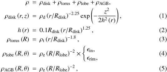 where the coordinates
  and (r,z) = (Rsinθ,Rcosθ) are the two-dimensional spherical and cylindrical coordinates. The disk and torus are placed in the regions where Rin ≤ R ≤ Rdisk and Rdisk ≤ R ≤ Rtorus, respectively. The most plausible definition of a disk should be a region where the matter is gravitationally bounded by the central star and has a Keplerian rotating motion. Although dusty disk structures have been spatially resolved in several evolved stars (e.g., Matsuura et al. 2006; Lykou et al. 2011), the dynamics are not well known or much less understood than accretion disks of young stellar objects. Therefore, we regarded the disk simply as a geometrically thin, optically thick dust structure. In Sect. 3.4 we show that such an inner disk is required in I16342.
The outer envelope consists of the bipolar lobe and spherical AGB shell. For the bipolar lobe, the regions  and
and  are the inner cavity and the rim of the lobe, respectively, where
 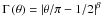 determines the lobe shape (see Oppenheimer et al. 2005). The AGB shell is placed outside the bipolar lobe with an outer boundary of Rout. The mass density coefficients are determined by the masses of the corresponding components. The dust mass is converted by assuming a gas-to-dust mass ratio of 200.
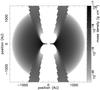 |
Fig. 3 Mass density map showing the inner 3000 AU region in a plane cutting through the symmetry axis. |
Figure 3 shows the mass density map in the inner 3000 × 3000 AU region. Our modeled geometry is complicated and it is in essence impossible to determine all parameters accurately from our observational data. Therefore, some parameters are set to be fixed values. Important parameters such as the inner disk radius Rdisk, the disk mass Mdisk, the torus radius Rtorus, and the torus mass Mtorus are estimated from our radiative transfer calculations.
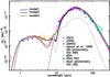 |
Fig. 4 Comparison of SEDs. Black lines are the result of the model with an inner disk. The solid, dotted, and dash-dot lines denote the total flux, the scattered light, and the thermal emission, respectively. Red and blue lines denote the results of the same geometry form but the disk mass of 0 and a model with only a torus with an inner radius of 500 AU. Colored dots are collected from previous observations: US Naval Observatory (USNO), the HST Guide Star Catalog (GSC)-II, 2MASS all-sky catalog of point source, Catalog of Infrared Observations, Edition 5 (Gezari et al. 1999), ISO photometry, SWS and LWS, MSX infrared point source catalog, IRAS point source catalog, and Akari/IRC mid-IR all-sky Survey (Ishihara et al. 2010). |
3.3. Dust particles
Dijkstra et al. (2003) discussed the mineralogy of I16342 based on their ISO spectra obtained using the Short Wavelength Spectrometer (SWS). Their data show a variety of absorption and emission features attributed to amorphous and crystalline silicate, frostetite, crystalline water ice, etc. Investigating the dust chemistry is one of the interesting and important tasks in dust formation of evolved stars. However, a thorough treatment of so many different chemical compositions and identification of the spatial distributions of individual species are very complicated tasks and are, therefore, beyond the scope of this paper. In our modeling, we adopted simple dust models. We used the optical constants for oxygen-deficient silicate (Ossenkopf et al. 1992).
We assumed different particle sizes for the outer envelope, the torus, and the inner disk, but the same sizes for the bipolar lobes and AGB shell. The particle size in the outer envelope was estimated with the polarization data. Since the polarizations are high and do not change much in the H- and KS-bands, the fraction of small particles is expected to be higher than that of the interstellar population. In our separated paper (Murakawa et al. 2012), we found a similar result in PPN I18276 and that a size distribution function with a steep power index provides a good estimate: 0.05 μm ≤ a and 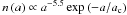 , where ac is the cut-off size (Kim et al. 1994). In I16342, ac = 5.0 μm fits the H and KS band polarizations.
Although large grains are expected in the disk and torus, we do not have (sub-)millimeter flux data or their gas masses and therefore we cannot constrain the sizes. Therefore, we provisionally adopted a size distribution of 0.005 μm ≤ a ≤ amax μm and  (Mathis et al. 1977). amax for the disk and torus are set to be 100 μm and 10 μm, respectively. We will not discuss dust growth in this object with our results.
3.4. Results
Table 2 lists the parameters of the selected model. Figure 4 shows the SEDs. The black lines are the result of the selected model (model 1). The viewing angle was chosen to be 30° measured from the equatorial plane. Although this result is slightly different compared to that (40°) estimated by Sahai et al. (1999), this discrepancy is not important in the following discussion. The model result fits the observation well from the optical to FIR, except for the 10 μm silicate absorption feature.
Parameters of our radiative transfer modeling.
We justify the presence of a geometrically thin, inner disk. First, we compared with a model without an inner disk (model 2), in which Mdisk is set to be 0 and the other parameters are identical. The difference is obvious in the wavelength range between 3 μm and 10 μm. Although the disk mass in model 1 is only 0.01 M⊙, the MIR flux is governed by the thermal emission from the hot dust in the inner disk. The other consideration is a model without an inner disk where we tried to fit the observations as best we can (model 3). This is our first attempt in the modeling (see Sect. 3.2). We find that models with small inner radii (a few tens AU) show too strong thermal emission at 3 μm to 10 μm and that a model with a large radius of Rin = 500 AU and Mtorus = 2.0 M⊙ fits best. However, as Fig. 4 shows, the flux between 3 μm to 6 μm is too low and model 1 fits better. The interpretation of I16342’s inner region is summarized as follows. An optically and geometrically thick torus should exist, as previous observations have shown. The torus is expected to have a large inner radius (a few hundred AU) and a high mass (1 M⊙). An additional inner geometrically thin disk is required, which is responsible for the thermal emission in the 3 μm to 10 μm.
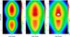 |
Fig. 5 Results of our two-dimensional radiative transfer calculations. The wavelengths are the 1.25 μm (J-band), 1.65 μm (H-band), and 2.05 μm (KS-band) from the left panels. The color scale bar indicate the surface brightness in W m-2 μm-1 arcsec-2. The Moffat PSF model images are convolved (see Sect. 2.1). |
Figure 5 shows the monochromatic model images at 1.25 μm (J-band), 1.65 μm (H-band), and 2.05 μm (KS-band) from left to right, which are simulated by scattering and absorption only. In these images, the Moffat PSF model images (see Sect. 2.1) are convolved. We confirmed that the Gaussian PSF convolution produces a centro-symmetric polarization pattern in the bipolar lobe, but the vectors are aligned with the Moffat PSF model. This is quite understandable because the surface brightness of a Gaussian function decays much faster than a Moffat function. The vector alignment in the entire nebula is reproduced by the PSF smoothing effect. Compared with the observations, the striking bipolar appearance and the presence of a dark lane in the equatorial plane are well reproduced. Although we do not present the results, we also confirmed that our model image in the 11.85 μm shows a bipolar appearance, as seen in the results of Verhoelst et al. (2009) and Lagadec et al. (2011).
4. Discussion
The mechanisms of PN shaping have been discussed in a number of publications before. To form a striking bipolarity with an equatorial narrow waist, the mass loss material should be highly concentrated in the equatorial plane. Morris (1987) modeled mass loss in a binary system from the primary red giant. Depending on the physical conditions, e.g. the mass and the separation of the secondary, a part of the mass loss material from the primary can be transferred onto the secondary, which forms a circum-companion disk. A part of accreting matter can be blown along the polar direction as a jet. Many bipolar PNs and PPNs, presumably I16342 too, are thought to form by the binary interaction based on this idea. Both theories and observations have developed the binary interaction hypothesis.
Silicate carbon stars are objects in which oxygen-rich species exist around carbon stars. According to the current interpretation of the dual chemistry, the silicate dust that was ejected when the central star was an M giant is stored in a disk around the hypothetical binary companion and then the central star is transformed into a carbon star through the third dredge-up (Lloyd-Evans 1990). V778 Cyg is an object of this class, which shows the 10 μm silicate emission feature, see Yamamura et al. (2000). These authors found that the dust has sub-micron sizes and temperatures of 300 − 600 K and is located at about 24 AU from the primary. The present-day mass-loss rate is estimated to be about 10-8 M⊙ yr-1. They interpret that the mass loss material can be trapped in the circum-companion disk, but leaves soon after within a few orbital periods because the disk is optically thin and the dust is blown away by the strong radiation pressure from the primary. With these low mass-loss rates, the disks are unlikely to be responsible for a bipolar appearance. It is of interest to mention the results of the smoothed particle hydrodynamic simulations for high mass-loss rate cases of ≳ 10-5 M⊙ yr-1 by Mastrodemos & Morris (1998, 1999,hereafter M98 and M99). Their simulations assumed a mass-losing AGB primary and a main-sequence companion (MS = 0.25 − 2 M⊙) with orbital separations of 3.6 − 50 AU. In M 1, 2, 10, 12, and 15 out of their 18 models, the density ratios of the equator to the pole ρeq/ρpol exceeds ~ 10 and the nebulae are classified as bipolar. M 1 and 2 are extreme cases, where the separations of the companion is small (6.3 AU in their models) and ratios of the accretion rate to the mass-loss rate are as high as ~ 0.1, yielding Ṁacc ≳ 10-6 M⊙ yr-1. ρeq/ρpol exceeds 100. These systems are likely to be progenitors of bipolar PNs with narrow waists. The thick winds sufficiently shield the strong radiation from the primary and the mass loss matter is stabilized there for a long time (Yamamura et al. 2000; Soker 2000), as expected in the Red Rectangle (Jura et al. 1995; van Winckel et al. 1998), AFGL 2688 (e.g., Bieging & Nguyen-Q-Rieu 1996), and probably I16342.
We now consider a simple model of AGB mass loss to see the competition of the radiation and the shielding based on a similar concept to “equatorial back-flow” introduced by Soker (2000). We assumed that a dust particle is directly irradiated by the radiation from the central star. The ratio of the radiation pressure to the gravitational attraction βdust is given by βdust = L ⋆ Crp/4πGM ⋆ c, where Crp is the cross section of the radiation pressure per unit mass, G the gravity constant and c the velocity of light. Applying the stellar parameters of L ⋆ = 6000 L⊙ and M ⋆ = 1 M⊙, a dust model that is derived from the outer envelope in our modeling, Crp = 6.73 × 103 cm2 g-1, where the stellar flux is assumed to dominate at λ = 1 μm, βdust is found to be ~ 3 × 10³. This high value is quite reasonable in AGB winds, where the dust is blown away by the radiation pressure. Next, the shielding by the mass loss ejecta is considered. We assumed a spherically symmetric mass loss at a constant Ṁ and constant radial expansion velocity Vr. The mass density has a power law distribution  , where r is the distance from the central star. The optical depth between the inner boundary (r = Rin) and a position at r = R is given by
 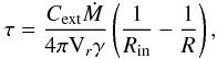 (6)where Cext is the extinction cross section per unit mass of the dust and γ the gas-to-dust mass ratio of 200. If the mass-loss rate reaches 10-5 M⊙ yr-1 at an expansion velocity of 15 km s-1, and R ≫ Rin = 5 AU is assumed, we derive an optical depth
 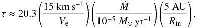 (7)where Cext = 9.10 × 103 cm2 g-1. The dust shell is optically thick. When dust particles move away, the radiation is shielded by the dust that is formed by the subsequent mass loss event. The optical depth attains ~8.0 ( = lnβdust) at R ~ 8.3 AU and the attenuated βdust values becomes ~1. The radiation pressure force cannot govern the motion of the particles. If the system has a close binary, the gravitational attraction of the secondary can affect the motion of the mass loss ejecta and can concentrate the flow toward the orbital plane. This leads to a flatter geometry, i.e. disk.
We have a rough scenario of the inner part of I16342’s CDS as follows. The inner disk of I16342 in our model, which is introduced to be responsible for the MIR flux, is a circum-companion or circum-binary disk that is formed by this mechanism. Because the optical depth of the disk is so high at ~ 400 in the V-band that the effect of the radiation is negligible, the disk can be gravitationally bounded by the central star(s). On the other hand, the torus is formed in a somewhat different way. If we assumed that I16342 has a binary companion, an angular momentum that is supplied by a close companion (say MS ~ 1 M⊙) is insufficient for the entire torus to have a keplerian rotating motion. Therefore, the torus is probably a structure that is accumulated from dust that is escaping from the central star(s).
5. Conclusion
We modeled the CDS of the WFS IRAS 16342–3814 with two-dimensional radiative transfer calculations. The model parameters were constrained by fitting the SED collected from various sources and the polarization images obtained using the VLT/NACO instrument. I16342 shows a striking bipolar appearance from the optical to the MIR wavelength ranges. Taking into account a large viewing angle of 30° − 40°, an optically thick dust torus structure is expected in the equatorial plane. We first tried to fit a model consisting of a geometrically thick torus and an outer envelope with bipolar lobes and a spherical AGB shell. However, these models cannot reproduce the SED and the bipolar appearance simultaneously. We found that an additional component of an optically thick, geometrically thin disk is required inside the torus. In our modeling, different dust sizes were assumed for the disk, the torus, and the outer envelope. The particle sizes in the outer envelope were estimated from the polarization data. The polarization reaches 25 − 38% in the H band and 20 − 38% in the KS band in our observations. This weak wavelength dependence is explained with a steeper power index of − 5.5 of the size distribution function than that of − 3.5 for the ISM. Similar results are found in some other PPNs. Because of the submillimeter and millimeter flux information and the estimation of the disk are missing, the particle sizes of these component cannot be constrained well. We adopted dust models of amax = 100 μm for the disk and amax = 10 μm for the torus. With this assumption, the masses of these components were determined to be 0.01 M⊙ and 1 M⊙, respectively, but have large uncertainties.
We discussed a possible formation scenario for the disk and torus. The important factors are the mass-loss rate and the binary interaction. For low- to intermediate-rates, the system is likely to have an optically thin circum-companion disk. To form an optically thick disk, the mass-loss rate would need to be so high that the thick wind blocks the radiation from the primary. This allows a part of the mass loss ejecta to be condensed in the equatorial region and to stay there for a long time. The remains, which are leaving from the central star(s), form the torus.
Acknowledgments
The NIR polarimetric images were obtained at the European Southern Observatory (proposal ID: 383.D-0197). The photometric and spectroscopic data are data produces from the Two Micron All Sky Survey, which is a joint project of the University of Massachusetts and the Infrared Processing and Analysis Center/California Institute of Technology, funded by the National Aeronautics and Space Administration and the National Science Foundation, AKARI, a JAXA project with the participation of ESA, Infrared Space Observatory, and Infrared Astronomical Satellite. We thank Luke T. Maud for his encouraging discussions and proofreading of the paper.
References
- Balick, B., Preston, H. L., & Icke, V. 1987, AJ, 94, 1641 [NASA ADS] [CrossRef] [Google Scholar]
- Bendinelli, O., Zavatti, F., Parmeggiani, G., et al. 1990, AJ, 99, 774 [NASA ADS] [CrossRef] [Google Scholar]
- Bieging, J. H., & Nguyen-Q-Rieu 1996, AJ, 112, 706 [NASA ADS] [CrossRef] [Google Scholar]
- Bjorkman, J. E., & Cassinelli, J. P. 1993, ApJ, 409, 429 [NASA ADS] [CrossRef] [Google Scholar]
- Claussen, M. J., Sahai, R., & Morris, M. 2009, ApJ, 691, 219 [NASA ADS] [CrossRef] [Google Scholar]
- Dijkstra, C., Waters, L. B. F. M., Kemper, F., et al. 2003, A&A, 399, 1037 [NASA ADS] [CrossRef] [EDP Sciences] [Google Scholar]
- Gezari, D. Y., Pitts, P. S., & Schmitz, M. 1999, VizieR On-line Data Catalog: II/225 [Google Scholar]
- Gómez, J. F., Ricardo Rizzo, J., Suárez, O., et al. 2011, ApJ, 739, L14 [NASA ADS] [CrossRef] [Google Scholar]
- He, J.-H., Imai, H., Hasegawa, T. I., et al. 2008, A&A, 488, L21 [NASA ADS] [CrossRef] [EDP Sciences] [Google Scholar]
- Hrivnak, B. J., Kwok, S., & Volk, K. M. 1989, ApJ, 346, 265 [NASA ADS] [CrossRef] [Google Scholar]
- Icke, V. 1988, A&A, 202, 177 [NASA ADS] [Google Scholar]
- Imai, H. 2007, in Astrophysical Masers and their Environments, eds. J. M. Chapman, & W. A. Baan (Cambridge: Cambridge University Press), IAU Symp., 242, 279 [Google Scholar]
- Imai, H., Chong, S. N., He, J.-H., et al. 2012, PASJ, in press [Google Scholar]
- Ishihara, D., Onaka, T., Kataza, H., et al. 2010, A&A, 514, A1 [NASA ADS] [CrossRef] [EDP Sciences] [Google Scholar]
- Jura, M., Balm, S. P., & Kahane, C. 1995, ApJ, 453, 721 [NASA ADS] [CrossRef] [Google Scholar]
- Kahane, C., Barnbaum, C., Uchida, K., Balm, S. P., & Jura, M. 1998, ApJ, 500, 466 [NASA ADS] [CrossRef] [Google Scholar]
- Kahn, F. D., & West, K. A. 1985, MNRAS, 212, 837 [NASA ADS] [CrossRef] [Google Scholar]
- Kim, S.-H., Martin, P. G., & Hendry, P. D. 1994, ApJ, 422, 164 [NASA ADS] [CrossRef] [Google Scholar]
- Kwok, S. 1982, ApJ, 258, 280 [NASA ADS] [CrossRef] [Google Scholar]
- Kwok, S. 1993, ARA&A, 31, 63 [NASA ADS] [CrossRef] [Google Scholar]
- Lagadec, E., Verhoelst, T., Mékarnia, D., et al. 2011, MNRAS, 417, 32 [NASA ADS] [CrossRef] [Google Scholar]
- Likkel, L., & Morris, M. 1988, ApJ, 329, 914 [NASA ADS] [CrossRef] [Google Scholar]
- Lloyd-Evans, T. 1990, MNRAS, 243, 336 [NASA ADS] [Google Scholar]
- Lykou, F., Chesneau, O., Zijlstra, A. A., et al. 2011, A&A, 527, A105 [NASA ADS] [CrossRef] [EDP Sciences] [Google Scholar]
- Mastrodemos, N., & Morris, M. 1998, A&A, 497, 303 (M98) [Google Scholar]
- Mastrodemos, N., & Morris, M. 1999, A&A, 523, 357 (M99) [Google Scholar]
- Mathis, J. S., Rumple, W., & Nordsieck, K. H. 1977, ApJ, 217, 425 [NASA ADS] [CrossRef] [Google Scholar]
- Matsuura, M., Chesneau, O., Zijlstra, A. A., et al. 2006, ApJ, 646, L123 [NASA ADS] [CrossRef] [Google Scholar]
- Meixner, M., Ueta, T., Dayal, A., et al. 1999, ApJS, 122, 221 [NASA ADS] [CrossRef] [Google Scholar]
- Moffat, A. F. J. 1996, A&A, 3, 455 [Google Scholar]
- Morris, M. 1987, PASP, 99, 1115 [NASA ADS] [CrossRef] [Google Scholar]
- Murakawa, K., Preibisch, T., & Kraus, S., et al. 2008a, A&A, 490, 673 [NASA ADS] [CrossRef] [EDP Sciences] [Google Scholar]
- Murakawa, K., Ohnaka, K., Driebe, T., et al. 2008b, A&A, 489, 195 [NASA ADS] [CrossRef] [EDP Sciences] [Google Scholar]
- Murakawa, K., Ueta, T., & Meixner, M. 2010a, A&A, 510, A30 [NASA ADS] [CrossRef] [EDP Sciences] [Google Scholar]
- Murakawa, K., Oudmaijer, R., & Izumiura, H. 2012, A&A, submitted [Google Scholar]
- Oppenheimer, B. D., Bieging, J. H., Schmidt, G. D., et al. 2005, ApJ, 624, 957 [NASA ADS] [CrossRef] [Google Scholar]
- Ossenkopf, V., Henning, Th., & Mathis, J. S. 1992, A&A, 261, 567 [NASA ADS] [Google Scholar]
- Sahai, R., & Trauger, J. T. 1998, AJ, 116, 1357 [NASA ADS] [CrossRef] [Google Scholar]
- Sahai, R., te Lintel Hekkert, P., Morris, M., Zijlstra, A., & Likkel, L. 1999, ApJ, 514, L115 [NASA ADS] [CrossRef] [Google Scholar]
- Sahai, R., Le Mignant, D., Sánchez Contreras, C., Campbell, R. D., & Chaffee, F. H. 2005, ApJ, 622, L53 [NASA ADS] [CrossRef] [Google Scholar]
- Soker, N. 2000, MNRAS, 312, 217 [NASA ADS] [CrossRef] [Google Scholar]
- Soker, N., & Livio, M. 1989, ApJ, 339, 268 [NASA ADS] [CrossRef] [Google Scholar]
- Suárez, O., Gómez, J. F., Miranda, L. F., et al. 2009, A&A, 505, 217 [NASA ADS] [CrossRef] [EDP Sciences] [Google Scholar]
- Ueta, T., & Meixner, M. 2003, ApJ, 586, 1338 [NASA ADS] [CrossRef] [Google Scholar]
- van der Veen, W. E. C. J., Habing, H. J., & Geballe, T. R. 1989, A&A, 226, 108 [NASA ADS] [Google Scholar]
- van Winckel, H., Waelkens, C., Waters, L. B. F. M., et al. 1998, A&A, 336, L17 [NASA ADS] [Google Scholar]
- Verhoelst, T., Waters, L. B. F. M., Verhoeff, A., et al. 2009, A&A, 503, 837 [NASA ADS] [CrossRef] [EDP Sciences] [Google Scholar]
- Walsh, A. J., Breen, S. L., Bains, I., & Vlemmings, W. H. T. 2009, MNRAS, 394, L70 [NASA ADS] [Google Scholar]
- Whittet, D. C. B., Martin, P. G., Hough, J. H., et al. 1992, ApJ, 386, 562 [NASA ADS] [CrossRef] [Google Scholar]
- Witzel, G., Eckart, A., Buchholz, R. M., et al. 2011, A&A, 525, 130 [Google Scholar]
- Yamamura, I., Dominik, C., & de Jong, T. 2000, A&A, 363, 629 [NASA ADS] [Google Scholar]
- Zijlstra, A. A., Chapman, J. M., te Lintel Hekkert, P., et al. 2001, MNRAS, 322, 280 [NASA ADS] [CrossRef] [Google Scholar]
- Zuckerman, B., & Lo, K. Y. 1987, A&A, 173, 263 [NASA ADS] [Google Scholar]
All Tables
All Figures
|
Fig. 1 Radial plot of the PSFs in the J (red), H (green), and KS (blue) bands. The surface brightnesses are normalized. The observations are compared with the two one-dimensional PSF models of Moffat and Gaussian functions. |
| In the text | |
|
Fig. 2 J, H, and KS band images of IRAS 16342–3814 obtained using NACO on the VLT. The polarization vector lines are overlaid on the H and KS band images. The field of view is |
| In the text | |
|
Fig. 3 Mass density map showing the inner 3000 AU region in a plane cutting through the symmetry axis. |
| In the text | |
|
Fig. 4 Comparison of SEDs. Black lines are the result of the model with an inner disk. The solid, dotted, and dash-dot lines denote the total flux, the scattered light, and the thermal emission, respectively. Red and blue lines denote the results of the same geometry form but the disk mass of 0 and a model with only a torus with an inner radius of 500 AU. Colored dots are collected from previous observations: US Naval Observatory (USNO), the HST Guide Star Catalog (GSC)-II, 2MASS all-sky catalog of point source, Catalog of Infrared Observations, Edition 5 (Gezari et al. 1999), ISO photometry, SWS and LWS, MSX infrared point source catalog, IRAS point source catalog, and Akari/IRC mid-IR all-sky Survey (Ishihara et al. 2010). |
| In the text | |
|
Fig. 5 Results of our two-dimensional radiative transfer calculations. The wavelengths are the 1.25 μm (J-band), 1.65 μm (H-band), and 2.05 μm (KS-band) from the left panels. The color scale bar indicate the surface brightness in W m-2 μm-1 arcsec-2. The Moffat PSF model images are convolved (see Sect. 2.1). |
| In the text | |
Current usage metrics show cumulative count of Article Views (full-text article views including HTML views, PDF and ePub downloads, according to the available data) and Abstracts Views on Vision4Press platform.
Data correspond to usage on the plateform after 2015. The current usage metrics is available 48-96 hours after online publication and is updated daily on week days.
Initial download of the metrics may take a while.