© ESO, 2012

1. Introduction

The supersonic nonthermal motions observed in molecular clouds have been attributed to the presence of magnetohydrodynamic (MHD) waves of sub-Alfvénic amplitudes (Arons & Max 1975), of which the Alfvén waves are the longest-lived (Zweibel & Josafatsson 1983). Indeed, molecular clouds and the cores embedded in them are threaded by the Galactic magnetic field, as revealed by polarization maps of the thermal dust emission (see e.g. Tang et al. 2009).

Molecular cloud cores, the sites of star formation, are characterized by velocity dispersions with nonthermal motions subsonic and uniform, in contrast to the surrounding lower density gas, where nonthermal motions are supersonic and in general increasing with size (Barranco & Goodman 1998; Goodman et al. 1998; Caselli et al. 2002). The NH₃ observations by Pineda et al. (2010) of the B5 region in Perseus revealed that the transition in velocity dispersion between the quiescent core and its more “turbulent” environment is sharp, taking place in a thin layer with a width of less than 0.04 pc.

Several groups have performed simulations and developed (semi)analytical models of the propagation of non-linear and linear Alfvén waves in interstellar clouds, but the main focus of these studies was either on the generation of density fluctuations and velocity dispersions with properties comparable to those of molecular clouds (Heitsch & Burkert 2002; Kudoh & Basu 2003, 2006), or on the role of internally generated Alfvén waves to support clumps within molecular clouds against their own self-gravity, taking into account the ionization structure and the ion-neutral drift (Martin et al. 1997; Coker et al. 2000). Our main objective is to study how density gradients, ionization fraction and non-linear wave interaction affect the propagation and the amplitude of Alfvén waves at the small scale of the interface between a dense core and its environment.

For this goal, we considered a simple one-dimensional cloud model for which the propagation of Alfvén waves is formulated in terms of Elsässer variables. This formulation allows one to treat propagation, reflection, damping, and nonlinear interactions in a simpler form compared to the original fluid equations (Elsässer 1950; Dobrowolny et al. 1980; Marsch & Mangeney 1987). Our approach is similar to that adopted for studying the propagation and reflection of Alvén waves in radially stratified stellar atmospheres and winds (Velli 1993). In this context the density gradients have the main effect of modulating the amplitude of Alfvén waves. This may affect the damping that results from the ion-neutral drift and at the same time trigger the development of a (perpendicular) turbulent cascade. Here we will focus mostly on the first aspect, although we will also use a phenomenological model to describe the dissipation of turbulence (successfully applied to the solar wind, e.g. Verdini et al. 2010) to see how it affects the results.

The paper is organized as follows: in Sect. 2 we derive the wave equation and review the conditions for wave propagation; in Sect. 3 we formulate the problem in terms of Elssässer variables; in Sect. 4 we describe the method of solution; we discuss some special cases in Sect. 5 and, in Sect. 6, we consider wave propagation, damping and reflection in a one-dimensional cloud model with a specific density and ionization profile; we evaluate the energy dissipation due to both ion-neutral drift and nonlinear effects; finally in Sect. 7 we summarize our conclusions.

2. Wave equation and dispersion relation

We considered a one-dimensional density distribution ρ(x), threaded by a magnetic field ${B}\mathrm{=}\mathit{B}\hat{{x}}$, in which the field is stationary and uniform, the latter condition resulting from the requirement of zero divergence, ∇·B = 0. The total density of the gas ρ is the sum of the densities of neutrals (ρ_n), ions (ρ_i) and electrons (ρ_e), and we assumed that the gas is electrically neutral. For applications to molecular clouds, we assumed that the field is frozen in the ions, which transfer momentum to the neutrals via elastic collisions. We neglected the electron’s inertia and focused on the ambipolar diffusion regime (see e.g. Pinto et al. 2008), ignoring Hall and Ohmic diffusion. In the regime of interest in this work (n(H₂) ~ 10⁴–10⁵ cm^-3, B ~ 10–100 μG), Ohmic diffusion is about 10 orders of magnitudes smaller than ambipolar diffusion and can be safely neglected; on the other hand, Hall diffusion is about one order of magnitude smaller than ambipolar diffusion, for standard grain size distribution, and about 4 orders of magnitudes smaller in the case of large (micron size) dust grains (see, e.g., Wardle & Ng 1999; Nakano et al. 2002; Pinto et al. 2008). The consequences of the Hall effect on the propagation of Alfvén waves in non-homogeneous media have been considered by Campos & Isaeva (1993).

In our analysis, we also assumed that the magnetic force is transferred to the neutrals only by collisions with ions. Actually, in the density regime of interest, charged dust grains can contribute as much as ions in the frictional force, provided that a population of small ( ≲ μm size) grains is present (Nakano et al. 2002). If only large ( ≳ μm size) grains are present, as expected if some amount of dust coagulation has taken place (Ormel et al. 2009), the contribution of grains to the frictional force becomes much smaller. On the other hand, large-size dust grains may induce dispersive effects on the propagation of nonlinear magnetic disturbances, and even promote the formation of soliton structures, although on scales at best one order of magnitude smaller than the typical size of a molecular cloud core (Pandey et al. 2008).

We considered transverse disturbances that are characterized by magnetic field b and velocities u_n and u_i (the latter were also assumed to be incompressible). We assumed that the sources of the waves are located at sufficiently large distance from the core’s midplane to neglect their density-pressure feedback on the cloud. The equations of motion and the induction equation read $\begin{array}{ccc}& & \\ & & {\mathit{\rho }}_{\mathrm{i}}\frac{\mathit{\partial }{u}\mathrm{i}}{\mathit{\partial t}}\mathrm{-}\frac{\mathit{B}}{\mathrm{4}\mathit{\pi }}\frac{\mathit{\partial }{b}}{\mathit{\partial x}}\mathrm{-}{\mathit{\gamma }}_{\mathrm{in}}{\mathit{\rho }}_{\mathrm{i}}{\mathit{\rho }}_{\mathrm{n}}\mathrm{(}{u}\mathrm{n}\mathrm{-}{u}\mathrm{i}\mathrm{)}\mathrm{=}\mathrm{-}{\mathit{\rho }}_{\mathrm{i}}{u}\mathrm{i}\mathrm{·}{\mathrm{\nabla }}_{\mathrm{\perp }}{u}\mathrm{i}\mathrm{-}\frac{\mathrm{1}}{\mathrm{8}\mathit{\pi }}{\mathrm{\nabla }}_{\mathrm{\perp }}\mathrm{|}{b}{\mathrm{|}}^{\mathrm{2}}\\ & & \\ & & \end{array}$\arraycolsep1.75ptwhere ${\mathit{\gamma }}_{\mathrm{in}}\mathrm{=}\frac{\mathrm{⟨}\mathit{\sigma w}{\mathrm{⟩}}_{\mathrm{in}}}{{\mathit{m}}_{\mathrm{i}}\mathrm{+}{\mathit{m}}_{\mathrm{n}}}\mathit{,}$(4)is the collisional drag coefficient,  ⟨ σw ⟩ _in is the momentum transfer rate coefficient, and ∇ _⊥  is the gradient along the direction perpendicular to the large-scale field B. On the right-hand side we have grouped the nonlinear terms: note that because of the assumption of transverse fluctuations they involve only gradients in that direction.

Combining the linearized Eqs. (1)–(3), we obtain the wave equation for u_i, $\frac{{\mathit{\partial }}^{\mathrm{3}}{u}\mathrm{i}}{\mathit{\partial }{\mathit{t}}^{\mathrm{3}}}\mathrm{-}{\mathit{V}}_{\mathrm{Ai}}^{\mathrm{2}}\frac{{\mathit{\partial }}^{\mathrm{3}}{u}\mathrm{i}}{\mathit{\partial }{\mathit{x}}^{\mathrm{2}}\mathit{\partial t}}\mathrm{+}{\mathit{\gamma }}_{\mathrm{in}}{\mathit{\rho }}_{\mathrm{n}}\left(\frac{\mathit{\rho }}{{\mathit{\rho }}_{\mathrm{n}}}\frac{{\mathit{\partial }}^{\mathrm{2}}{u}\mathrm{i}}{\mathit{\partial }{\mathit{t}}^{\mathrm{2}}}\mathrm{-}{\mathit{V}}_{\mathrm{An}}^{\mathrm{2}}\frac{{\mathit{\partial }}^{\mathrm{2}}{u}\mathrm{i}}{\mathit{\partial }{\mathit{x}}^{\mathrm{2}}}\right)\mathrm{=}\mathrm{0}\mathit{,}$(5)where ρ = ρ_n + ρ_i and V_Ai, V_An are the Alfvén velocities in the ions and the neutrals, respectively: ${\mathit{V}}_{\mathrm{Ai}}\mathrm{=}\frac{\mathit{B}}{\sqrt{\mathrm{4}\mathit{\pi }{\mathit{\rho }}_{\mathrm{i}}}}\mathit{,} {\mathit{V}}_{\mathrm{An}}\mathrm{=}\frac{\mathit{B}}{\sqrt{\mathrm{4}\mathit{\pi }{\mathit{\rho }}_{\mathrm{n}}}}\mathrm{·}$(6)Substituting in Eq. (5) a solution in the form u_i(x,t) = u_0iexp [i(kx − ωt)] , we obtain the well-known dispersion relation (DR) $\mathit{\omega }\mathrm{[}{\mathit{\omega }}^{\mathrm{2}}\mathrm{-}\mathrm{(}\mathit{k}{\mathit{V}}_{\mathrm{Ai}}{\mathrm{)}}^{\mathrm{2}}\mathrm{]}\mathrm{+}\mathrm{i}{\mathit{\gamma }}_{\mathrm{in}}\mathrm{[}\mathit{\rho }{\mathit{\omega }}^{\mathrm{2}}\mathrm{-}{\mathit{\rho }}_{\mathrm{i}}\mathrm{(}\mathit{k}{\mathit{V}}_{\mathrm{Ai}}{\mathrm{)}}^{\mathrm{2}}\mathrm{]}\mathrm{=}\mathrm{0}\mathit{,}$(7)first derived by Piddington (1956) and later by Kulsrud & Pearce (1969).

The amplitudes of the fluctuations in u_n and u_i are related to the amplitude of the fluctuations of b by ${u}\mathrm{0}\mathrm{n}\mathrm{=}\mathrm{-}{\mathit{V}}_{\mathrm{Ai}}\frac{\mathrm{i}{\mathit{\gamma }}_{\mathrm{in}}{\mathit{\rho }}_{\mathrm{i}}}{\mathit{\omega }\mathrm{+}\mathrm{i}{\mathit{\gamma }}_{\mathrm{in}}\mathit{\rho }}\left(\frac{\mathit{k}{\mathit{V}}_{\mathrm{Ai}}}{\mathit{\omega }}\right)\frac{{b}\mathrm{0}}{\mathit{B}}\mathit{,}$(8)and ${u}\mathrm{0}\mathrm{i}\mathrm{=}\mathrm{-}{\mathit{V}}_{\mathrm{Ai}}\frac{\mathit{\omega }\mathrm{[}\mathit{\omega }\mathrm{+}\mathrm{i}{\mathit{\gamma }}_{\mathrm{in}}\mathit{\rho }\mathrm{]}\mathrm{-}{\mathit{\gamma }}_{\mathrm{in}}^{\mathrm{2}}{\mathit{\rho }}_{\mathrm{i}}{\mathit{\rho }}_{\mathrm{n}}}{\mathrm{[}\mathit{\omega }\mathrm{+}\mathrm{i}{\mathit{\gamma }}_{\mathrm{in}}\mathit{\rho }\mathrm{]}\mathrm{(}\mathit{\omega }\mathrm{+}\mathrm{i}{\mathit{\gamma }}_{\mathrm{in}}{\mathit{\rho }}_{\mathrm{n}}\mathrm{)}}\left(\frac{\mathit{k}{\mathit{V}}_{\mathrm{Ai}}}{\mathit{\omega }}\right)\frac{{b}\mathrm{0}}{\mathit{B}}\mathrm{·}$(9)For ρ_i/ρ_n ≪ 1, there are two separated regimes of wave propagation: long waves (for $\mathit{k}{\mathit{V}}_{\mathrm{Ai}}\mathrm{\ll }\sqrt{{\mathit{\rho }}_{\mathrm{i}}\mathit{/}{\mathit{\rho }}_{\mathrm{n}}}{\mathit{\gamma }}_{\mathrm{in}}{\mathit{\rho }}_{\mathrm{n}}$) and short waves (for kV_Ai ≫ γ_inρ_n). The physical reason is that when the timescale for wave damping becomes shorter than the wave period, wave oscillation cannot occur. Short waves are high-frequency waves propagating at the ion’s Alfvén speed, damped by collisions with neutrals. In the short-wave regime, the ratio of the amplitudes of the velocity oscillations reduces to $\frac{\mathrm{\left|}{u}\mathrm{0}\mathrm{n}\mathrm{\right|}}{\mathrm{\left|}{u}\mathrm{0}\mathrm{i}\mathrm{\right|}}\mathrm{=}\frac{{\mathit{\gamma }}_{\mathrm{in}}{\mathit{\rho }}_{\mathrm{i}}}{\mathit{\omega }}\mathit{,}$(10)i.e. the neutrals are weakly coupled to the ions and their amplitude of oscillation is very small. Therefore, these waves cannot be responsible for the linewidths of neutral species observed in molecular clouds.

In the limit of long waves, the wave Eq. (5) becomes $\frac{{\mathit{\partial }}^{\mathrm{2}}{u}\mathrm{i}}{\mathit{\partial }{\mathit{t}}^{\mathrm{2}}}\mathrm{-}{\mathit{V}}_{\mathrm{A}}^{\mathrm{2}}\frac{{\mathit{\partial }}^{\mathrm{2}}{u}\mathrm{i}}{\mathit{\partial }{\mathit{x}}^{\mathrm{2}}}\mathrm{-}{\mathit{\eta }}_{\mathrm{AD}}\frac{{\mathit{\partial }}^{\mathrm{3}}{u}\mathrm{i}}{\mathit{\partial }{\mathit{x}}^{\mathrm{2}}\mathit{\partial t}}\mathrm{=}\mathrm{0}\mathit{,}$(11)where V_A is the Alfvén speed in the gas of neutrals and ions (of density ρ = ρ_n + ρ_i), and η_AD is the ambipolar diffusion resistivity ${\mathit{\eta }}_{\mathrm{AD}}\mathrm{=}\frac{{\mathit{B}}^{\mathrm{2}}}{\mathrm{4}\mathit{\pi }{\mathit{\gamma }}_{\mathrm{in}}\mathit{\rho }{\mathit{\rho }}_{\mathrm{i}}}\mathrm{·}$(12)In this regime, the DR of Eq. (7) reduces to ${\mathit{\omega }}^{\mathrm{2}}\mathrm{-}{\mathit{k}}^{\mathrm{2}}{\mathit{V}}_{\mathrm{A}}^{\mathrm{2}}\mathrm{+}\mathrm{i}{\mathit{\eta }}_{\mathrm{AD}}{\mathit{k}}^{\mathrm{2}}\mathit{\omega }\mathrm{=}\mathrm{0.}$(13)For the propagation and damping of Alfvén waves in a molecular cloud a description in terms of forced waves is appropriate. Indeed, there are several possible sources of hydromagnetic waves in a molecular cloud, such as gravitational collapse of smaller parts, large-scale non-radial oscillations of the cloud, radiation pressure from young stars, expansion of HII regions, stellar outflows (Arons & Max 1975). In this case, the DR should be considered as a quadratic equation for the wavenumber k (with real and imaginary part) as a function of the frequency ω (real). Defining a complex wave number k = ℜ(k) + iℑ(k), in the limit $\mathit{\omega }\mathrm{\ll }{\mathit{V}}_{\mathrm{A}}^{\mathrm{2}}\mathit{/}{\mathit{\eta }}_{\mathrm{AD}}$, we derive from the real and imaginary parts of the dispersion relation Eq. (13) the expressions $\mathrm{\Re }\mathrm{\left(}\mathit{k}\mathrm{\right)}\mathrm{\approx }\mathrm{\pm }\frac{\mathit{\omega }}{{\mathit{V}}_{\mathrm{A}}}\mathit{,} \mathrm{and} \mathrm{\Im }\mathrm{\left(}\mathit{k}\mathrm{\right)}\mathrm{\approx }\mathrm{\pm }\frac{{\mathit{\omega }}^{\mathrm{2}}}{\mathrm{2}{\mathit{V}}_{\mathrm{A}}^{\mathrm{3}}}{\mathit{\eta }}_{\mathrm{AD}}\mathit{.}$(14)The condition for wave propagation,  | ℜ(k) |  ≥  | ℑ(k) | , is satisfied only if the frequency of forcing is lower than a critical frequency ${\mathit{\omega }}_{\mathrm{cr}}\mathrm{=}\mathrm{2}{\mathit{V}}_{\mathrm{A}}^{\mathrm{2}}\mathit{/}{\mathit{\eta }}_{\mathrm{AD}}$, or, the wavelength is longer than a critical value λ_cr = πη_AD/V_A (Kulsrud & Pearce 1969). In the low-ionization regime typical of a molecular cloud, ρ ≈ ρ_n, the condition for wave propagation reduces to ω ≤ 2γ_inρ_i or, in terms of wavelength, to $\mathit{\lambda }\mathrm{\ge }{\mathit{\lambda }}_{\mathrm{cr}}\mathrm{=}\frac{{\mathit{\pi }}^{\mathrm{1}\mathit{/}\mathrm{2}}\mathit{B}}{\mathrm{2}{\mathit{\gamma }}_{\mathrm{in}}{\mathit{\rho }}_{\mathrm{n}}^{\mathrm{1}\mathit{/}\mathrm{2}}{\mathit{\rho }}_{\mathrm{i}}}\mathrm{=}\frac{\mathit{\pi }{\mathit{V}}_{\mathrm{A}}}{{\mathit{\gamma }}_{\mathrm{in}}{\mathit{\rho }}_{\mathrm{i}}}\mathrm{·}$(15)We selected the case of depleted clouds where all metal species are frozen onto grains and the dominant ions are H⁺ and H$\begin{array}{}\mathrm{+}\\ \mathrm{3}\end{array}$. In this case γ_in = 2.38 × 10¹⁴ g^-1 cm³ s^-1 (see Pinto & Galli 2008) and the mean mass of neutrals and ions are m_n = 2.33m_H and m_i = 3m_H, respectively. Inserting numerical values, we obtain 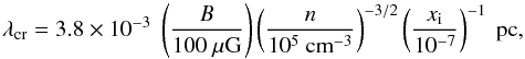${\mathit{\lambda }}_{\mathrm{cr}}\mathrm{=}\mathrm{3.8}\mathrm{\times }{\mathrm{10}}^{-3} \left(\frac{\mathit{B}}{\mathrm{100} \mathit{\mu }\mathrm{G}}\right){\left(\frac{\mathit{n}}{{\mathrm{10}}^{\mathrm{5}} \mathrm{cm}-3}\right)}^{\mathrm{-}\mathrm{3}\mathit{/}\mathrm{2}}{\left(\frac{{\mathit{x}}_{\mathrm{i}}}{{\mathrm{10}}^{-7}}\right)}^{-1} \mathrm{pc}\mathit{,}$(16)where x_i = n_i/n is the ionization fraction. In the regime of long waves, the amplitudes of the velocity oscillations reduce to ${u}\mathrm{0}\mathrm{n}\mathrm{=}\mathrm{-}\frac{\mathit{k}{\mathit{V}}_{\mathrm{A}}^{\mathrm{2}}}{\mathit{\omega }}\frac{{b}\mathrm{0}}{\mathit{B}}\mathit{,} \mathrm{and} {u}\mathrm{0}\mathrm{i}\mathrm{=}\mathrm{-}\frac{\mathit{\omega }}{\mathit{k}}\frac{{b}\mathrm{0}}{\mathit{B}}\mathrm{·}$(17)Since  | k |  = ω/V_A to lowest order in $\mathrm{(}{\mathit{\eta }}_{\mathrm{AD}}\mathit{\omega }\mathit{/}{\mathit{V}}_{\mathrm{A}}^{\mathrm{2}}{\mathrm{)}}^{\mathrm{2}}$, the two velocity amplitudes are equal in modulus  | u_0n |  =  | u_0i |  = V_A | b₀ | /B. These long-wavelength Alfvén waves propagate with speed V_A in a well-coupled ion-neutral gas, and may be responsible for the observed linewidths of ionic and neutral species observed in molecular clouds.

3. Model equations

The condition for the propagation of long waves is equivalent to assume that neutrals and ions are well coupled (|u_i − u_n | /V_An ≪  | b | /B). With this condition, and the approximation ρ_i ≪ ρ_n, the ion velocity can be obtained from Eq. (2) as ${u}\mathrm{i}\mathrm{=}{u}\mathrm{n}\mathrm{+}\frac{{\mathit{\eta }}_{\mathrm{AD}}}{\mathit{B}}\frac{\mathit{\partial }{b}}{\mathit{\partial x}}\mathrm{+}\frac{{\mathit{\eta }}_{\mathrm{AD}}}{{\mathit{B}}^{\mathrm{2}}}{b}\mathrm{·}{\mathrm{\nabla }}_{\mathrm{\perp }}{b}\mathrm{-}\frac{{\mathit{\eta }}_{\mathrm{AD}}}{\mathrm{2}{\mathit{B}}^{\mathrm{2}}}{\mathrm{\nabla }}_{\mathrm{\perp }}\mathrm{|}{b}{\mathrm{|}}^{\mathrm{2}}\mathit{.}$(18)Upon substitution of the above equation into the induction Eq. (3) one obtains a quite complicated equation. To make it more tractable, still accounting for non-linear interactions, we adopted the following additional assumptions: i) fluctuations have small amplitudes (b/B ≈ u_n/V_a < 1), thus, when substituting Eq. (18) into (3) we expand the non-linear terms only to the second order (cubic terms are neglected); ii) the ambipolar diffusion coefficient varies on a scale much larger than all the other quantities do, thus we neglect terms involving its derivatives. Under these assumptions, the induction equation is of the form $\begin{array}{ccc}\frac{\mathit{\partial }{b}}{\mathit{\partial t}}\mathrm{=}\mathit{B}\frac{\mathit{\partial }{u}\mathrm{n}}{\mathit{\partial x}}\mathrm{+}{b}\mathrm{·}{\mathrm{\nabla }}_{\mathrm{\perp }}{u}\mathrm{n}\mathrm{-}{u}\mathrm{n}\mathrm{·}{\mathrm{\nabla }}_{\mathrm{\perp }}{b}& & \\ & & \end{array}$(19)We see that nonlinearities also appear in terms that contain the ambipolar diffusion coefficient (the last two terms), therefore we expect that the turbulent cascade is also affected by ion-neutral drift. In view of the simple phenomenology that we will use (Eq. (26)) to describe the dissipation of turbulence, we additionally simplified the equation by adopting an ordering of the parallel and perpendicular length scales, namely iii) λ_cr/ℓ _|  |  ≪ b/B ≪ ℓ _⊥ /ℓ _|  | , where ℓ _{|  | ,    ⊥}  are the typical sizes of parallel and perpendicular large scales. We thus obtain the final model equations: ${\mathit{\rho }}_{\mathrm{n}}\frac{\mathit{\partial }{u}\mathrm{n}}{\mathit{\partial t}}\mathrm{=}\frac{\mathit{B}}{\mathrm{4}\mathit{\pi }}\frac{\mathit{\partial }{b}}{\mathit{\partial x}}\mathrm{-}\frac{\mathrm{1}}{\mathrm{8}\mathit{\pi }}{\mathrm{\nabla }}_{\mathrm{\perp }}\mathrm{|}{b}{\mathrm{|}}^{\mathrm{2}}\mathrm{+}\frac{\mathrm{1}}{\mathrm{4}\mathit{\pi }}{b}\mathrm{·}{\mathrm{\nabla }}_{\mathrm{\perp }}{b}\mathrm{-}{\mathit{\rho }}_{\mathrm{n}}{u}\mathrm{n}\mathrm{·}{\mathrm{\nabla }}_{\mathrm{\perp }}{u}\mathrm{n}\mathit{,}$(20)and $\frac{\mathit{\partial }{b}}{\mathit{\partial t}}\mathrm{=}\mathit{B}\frac{\mathit{\partial }{u}\mathrm{n}}{\mathit{\partial x}}\mathrm{+}{\mathit{\eta }}_{\mathrm{AD}}\frac{\mathit{\partial }}{\mathit{\partial x}}\left(\frac{\mathit{\partial }{b}}{\mathit{\partial x}}\right)\mathrm{+}{b}\mathrm{·}{\mathrm{\nabla }}_{\mathrm{\perp }}{u}\mathrm{n}\mathrm{-}{u}\mathrm{n}\mathrm{·}{\mathrm{\nabla }}_{\mathrm{\perp }}{b}\mathit{.}$(21)Equations (20) and (21) can be conveniently expressed in terms of the Elsässer variables, ${z}\mathrm{\pm }\mathrm{=}{u}\mathrm{n}\mathrm{\mp }\frac{{b}}{\sqrt{\mathrm{4}\mathit{\pi }{\mathit{\rho }}_{\mathrm{n}}}}\mathit{,}$(22)by dividing Eq. (21) by $\sqrt{\mathrm{4}\mathit{\pi }{\mathit{\rho }}_{\mathrm{n}}}$, then adding and subtracting Eqs. (20) and (21): $\begin{array}{ccc}\frac{\mathit{\partial }{z}\mathrm{\pm }}{\mathit{\partial t}}\mathrm{\pm }{\mathit{V}}_{\mathrm{A}}\frac{\mathit{\partial }{z}\mathrm{\pm }}{\mathit{\partial x}}\mathrm{=}\mathrm{-}{z}\mathrm{\mp }\mathrm{·}{\mathrm{\nabla }}_{\mathrm{\perp }}{z}\mathrm{\pm }\mathrm{-}\frac{\mathrm{1}}{{\mathit{\rho }}_{\mathrm{n}}}{\mathrm{\nabla }}_{\mathrm{\perp }}{\mathit{P}}_{\mathrm{m}}\mathrm{\pm }\frac{{\mathit{V}}_{\mathrm{A}}^{\mathrm{\prime }}}{\mathrm{2}}\mathrm{(}{z}\mathrm{\pm }\mathrm{-}{z}\mathrm{\mp }\mathrm{)}& & \\ & & \mathrm{\pm }\frac{{\mathit{\eta }}_{\mathrm{AD}}}{\mathrm{2}}\mathrm{(}{z}\mathrm{\pm }\mathrm{-}{z}\mathrm{\mp }\mathrm{)}\left[\mathrm{2}{\left(\frac{{\mathit{V}}_{\mathrm{A}}^{\mathrm{\prime }}}{{\mathit{V}}_{\mathrm{A}}}\right)}^{\mathrm{2}}\mathrm{-}\frac{{\mathit{V}}_{\mathrm{A}}^{\mathrm{\prime \prime }}}{{\mathit{V}}_{\mathrm{A}}}\right]\mathrm{-}{\mathit{\eta }}_{\mathrm{AD}}\frac{{\mathit{V}}_{\mathrm{A}}^{\mathrm{\prime }}}{{\mathit{V}}_{\mathrm{A}}}\left(\frac{\mathit{\partial }{z}\mathrm{\pm }}{\mathit{\partial x}}\mathrm{-}\frac{\mathit{\partial }{z}\mathrm{\mp }}{\mathit{\partial x}}\right)\\ & & \end{array}$(23)The superscripts ′ and ′′ indicate first- and second-order spatial derivatives along the x direction and P_m is the magnetic pressure. The first two terms on the left-hand side represent the temporal and spatial wave propagation, respectively. On the right-hand side, the first two term account for non-linear interactions; the term proportional to ${\mathit{V}}_{\mathrm{A}}^{\mathrm{\prime }}$ describes the losses related to the presence of gradients in the Alfvén velocity and wave reflection; the terms proportional to η_AD are associated to the dissipation by ambipolar diffusion and combined effects of density gradients and ion-neutral drift. Because we assumed fluctuations to lie in the plane perpendicular to B, the gradient ∇ _⊥  involves only perpendicular scales. Given the high Reynolds numbers found in molecular clouds (R_m ≈ 10⁸, Myers & Khersonsky 1995), a perpendicular turbulent cascade is expected to develop. These non-linear couplings involve only counter-propagating waves. Note however that even if only one mode is present, say z ₊ , density gradients or ion-neutral drift ensure the presence of the other mode (z ₋ ) and hence the triggering of the cascade.

The hypotheses that we have adopted in deriving Eqs. (20), (21), (23) are summarized in the following ordering: $\frac{{\mathit{\lambda }}_{\mathrm{cr}}}{{\mathit{\ell }}_{\mathrm{\left|}\mathrm{\right|}}}\mathrm{\ll }\frac{\mathit{b}}{\mathit{B}}\mathrm{\ll }\frac{{\mathit{\ell }}_{\mathrm{\perp }}}{{\mathit{\ell }}_{\mathrm{\left|}\mathrm{\right|}}}\mathrm{\ll }\frac{{\mathit{\rho }}_{\mathrm{n}}}{{\mathit{\rho }}_{\mathrm{i}}}\mathrm{·}$(24)Note that the first inequality is a stronger constraint than the long wavelength condition Eq. (15), but in molecular clouds one typically finds that λ_cr/ℓ_|| ≈ η_AD/V_AL ≲ 0.06 (see Eq. (16)) and ρ_n/ρ_i ≳ 10⁷, therefore the above ordering is generally satisfied even for ℓ_⊥/ℓ_|| > 1. The condition b/B ≪ ℓ_⊥/ℓ_|| can be rewritten as τ_A/τ_NL < 1 where the Alfvén and non-linear timescales are given by τ_A = ℓ_||/V_A and τ_NL = ℓ_⊥/z_± (we assumed b/B ≈ u/V_A ≈ z_±/V_a). In other words, the equations are suited to describe weak turbulence. Our inequality is more stringent than τ_A/τ_NL ≪ B/b given in Galtier et al. (2002), which was used to build a cascade model. We will not attempt such a detailed description of the cascade for two reasons that are related to the inhomogeneity. It will be clear in the following that the density gradients couple counter-propagating waves. A first consequence is that the phase of oppositely propagating low-frequency waves cannot be considered as random anymore, preventing us from exploiting a phase averaging method at large scales to obtain the kinetic equations. Moreover, in the inhomogeneous case typical of the cloud-core systems, the density gradients act as semi-reflecting boundaries, which enhance the amplitudes, and therefore the cascade rate of large-scale modes. These low-frequency waves in which energy is accumulated pose a problem with the continuity of the low-frequency tail of the spectrum. Our nonlinear model is really only in the spirit of von Karman & Howarth (1938) (see also Mac Low 1999), where the large eddies control the dissipation rate and the specific mechanism for small-scale dissipation is not of central importance. Large-scale fluctuations control the cascade, and fast, small-scale dissipation mechanisms, whether collisional or not, act as passive absorbers of cascaded energy.

Another comment concerns the possibility of nonlinear compressible interactions and processes such as parametric decay. These interactions may play a role, but in a completely turbulent situations where fluctuations have completely random phases, the decay via these resonant processes is greatly reduced (Malara & Velli 1996). Consequently, the density fluctuations that are there will play a role via processes such as phase mixing/resonant absorption, and shock heating, but will not alter, except at shocks, the dominant nature of the energy cascade given by the dimensional model described below.

4. Numerical method

We first sought solutions in form of monochromatic waves for the linearized Eq. (23). This allowed us to show the role of interference between waves as produced by reflection and ambipolar diffusion (see Sect. 5). The numerical method is presented in the next section Sect. 4.1. Then we solved the full set of Eq. (23) in their time-dependent form, treating the non-linear interactions in a phenomenological way and considering fluctuations that are characterized by a steep frequency spectrum. The details of the numerical method and the phenomenology adopted are given in Sect. 4.2.

4.1. Time-independent scheme for linear equations

We neglected non-linear terms and hence the perpendicular structure of Alfvén waves. We sought solutions for monochromatic waves of the form z _± (x,t) = V_A0y _± (x)exp( − iωt). For a cloud of typical size L and density ρ₀, we can define a characteristic Alfvén speed ${\mathit{V}}_{\mathrm{A}\mathrm{0}}\mathrm{=}\mathit{B}\mathit{/}\sqrt{\mathrm{4}\mathit{\pi }{\mathit{\rho }}_{\mathrm{0}}}$ and Alfvén time t_A = L/V_A0, and the nondimensional variables ξ = x/L and $\begin{array}{}{}_{\mathrm{˜}}\\ \mathit{\rho }\end{array}\mathrm{=}\mathit{\rho }\mathit{/}{\mathit{\rho }}_{\mathrm{0}}$. In nondimensional form, Eq. (23) can be written as $\begin{array}{ccc}\mathrm{\pm }\frac{\mathrm{1}}{\stackrel{}{{{\mathit{\rho }}^{\mathrm{1}\mathit{/}\mathrm{2}}}_{\mathrm{˜}}}}{\mathit{y}}_{\mathrm{\pm }}^{\mathrm{\prime }}\mathrm{=}\mathrm{i}\mathit{W}{\mathit{y}}_{\mathrm{\pm }}\mathrm{\mp }\frac{\mathrm{1}}{\mathrm{4}}\left({\mathit{y}}_{\mathrm{\pm }}\mathrm{-}{\mathit{y}}_{\mathrm{\mp }}\right)\begin{array}{}\mathrm{⎧}\\ \mathrm{⎪}\\ \mathrm{⎪}\\ \mathrm{⎨}\\ \mathrm{⎪}\\ \mathrm{⎪}\\ \mathrm{⎩}\end{array}\frac{\stackrel{}{{{\mathit{\rho }}^{\mathrm{\prime }}}_{\mathrm{˜}}}}{\stackrel{}{{{\mathit{\rho }}^{\mathrm{3}\mathit{/}\mathrm{2}}}_{\mathrm{˜}}}}\mathrm{\pm }\begin{array}{}\mathrm{˜}\\ {\mathit{\eta }}_{\mathrm{AD}}\end{array}\left[\frac{\stackrel{}{{{\mathit{\rho }}^{\mathrm{\prime \prime }}}_{\mathrm{˜}}}}{\begin{array}{}\mathrm{˜}\\ \mathit{\rho }\end{array}}\mathrm{-}\frac{\mathrm{1}}{\mathrm{2}}{\left(\frac{\stackrel{}{{{\mathit{\rho }}^{\mathrm{\prime }}}_{\mathrm{˜}}}}{\begin{array}{}\mathrm{˜}\\ \mathit{\rho }\end{array}}\right)}^{\mathrm{2}}\right]\begin{array}{}\mathrm{⎫}\\ \mathrm{⎪}\\ \mathrm{⎪}\\ \mathrm{⎬}\\ \mathrm{⎪}\\ \mathrm{⎪}\\ \mathrm{⎭}\end{array}& & \\ & & \mathrm{+}\begin{array}{}\mathrm{˜}\\ {\mathit{\eta }}_{\mathrm{AD}}\end{array}\frac{\stackrel{}{{{\mathit{\rho }}^{\mathrm{\prime }}}_{\mathrm{˜}}}}{\mathrm{2}\begin{array}{}\mathrm{˜}\\ \mathit{\rho }\end{array}}\mathrm{(}{\mathit{y}}_{\mathrm{\pm }}^{\mathrm{\prime }}\mathrm{-}{\mathit{y}}_{\mathrm{\mp }}^{\mathrm{\prime }}\mathrm{)}\mathrm{+}\frac{\begin{array}{}\mathrm{˜}\\ {\mathit{\eta }}_{\mathrm{AD}}\end{array}}{\mathrm{2}}\mathrm{(}{\mathit{y}}_{\mathrm{\pm }}^{\mathrm{\prime \prime }}\mathrm{-}{\mathit{y}}_{\mathrm{\mp }}^{\mathrm{\prime \prime }}\mathrm{)}\mathit{,}\end{array}$(25)where W = ωL/V_A0 and $\begin{array}{}{}_{\mathrm{˜}}\\ {\mathit{\eta }}_{\mathrm{AD}}\end{array}\mathrm{=}{\mathit{\eta }}_{\mathrm{AD}}\mathit{/}\mathrm{\left(}{\mathit{V}}_{\mathrm{A}\mathrm{0}}\mathit{L}\mathrm{\right)}$. For uniform density ($\begin{array}{}{}_{\mathrm{˜}}\\ \mathit{\rho }\end{array}\mathrm{=}\mathrm{1}$) and without dissipation ($\begin{array}{}{}_{\mathrm{˜}}\\ {\mathit{\eta }}_{\mathrm{AD}}\end{array}\mathrm{=}\mathrm{0}$), Eq. (25) describes the propagation of Alfvén waves traveling to the right ( +  sign) and to the left ( −  sign).

Because ambipolar diffusion is a small effect in typical ISM conditions ($\begin{array}{}{}_{\mathrm{˜}}\\ {\mathit{\eta }}_{\mathrm{AD}}\end{array}\mathrm{\ll }\mathrm{1}$), we adopted a perturbational approach. We initially solved Eq. (25) guessing at a functional form for the second-order derivatives. In particular, we assumed the exponentially damped behavior predicted by analytical studies (we have verified that the numerical results are independent of the choice of the initial guess); then we used the second-order derivatives of the solutions obtained by the guess function to integrate Eq. (25) and obtained a new set of second-order derivatives. This procedure was iterated until convergence of the solution was attained.

Special care has to be taken when choosing boundary conditions suitable to describe waves incident on both sides of an interstellar cloud because of the interference between the incoming waves. When only ambipolar diffusion is present, the iterative procedure reduces the problem to a boundary-value problem for the fields z ^± . For wave propagation in a density gradient without dissipation, the boundary-value problem is well defined only when one wave vanishes at one boundary. In the more realistic case, where both modes are injected at the boundaries, solutions depend on the relative phase between the injected z _± . The phase in fact controls the interference between the incident wave and the reflected wave inside the density profile. We will describe in detail the appropriate initial conditions in the application to interstellar clouds (Sect. 6), first dealing with density gradients, then considering both ambipolar diffusion and density gradients.

4.2. Time-dependent scheme for non-linear equations

To evaluate the effect of turbulent dissipation, which can be triggered by non-linear wave interactions, we did not model the turbulent cascade. Instead we used a phenomenological expression (Dmitruk et al. 2001) that accounts for the damping of the waves and preserves the structure of non-linear terms, allowing interactions only among counter-propagating waves. We therefore integrated Eq. (23) modified with the following substitution in the RHS, $\mathrm{-}{z}\mathrm{\mp }\mathrm{·}{\mathrm{\nabla }}_{\mathrm{\perp }}{z}\mathrm{\pm }\mathrm{-}\frac{\mathrm{1}}{{\mathit{\rho }}_{\mathrm{n}}}{\mathrm{\nabla }}_{\mathrm{\perp }}{\mathit{P}}_{\mathrm{m}}\mathrm{\to }\mathrm{-}\frac{\mathrm{|}{z}\mathrm{\mp }\mathrm{|}{z}\mathrm{\pm }}{\mathrm{2}{\mathit{\ell }}_{\mathrm{\perp }}}\mathit{,}$(26)where ℓ _⊥  represents the dimension of the largest eddies (the energy containing scale in the turbulent field).

The form of the nonlinear term may be heuristically derived in the framework of reduced MHD in which variations along the perpendicular directions are decoupled from those along the magnetic field (∇ = ∇ _⊥  + ∇ _|  | , with ∇ _⊥  ≫ ∇ _|  | ). In presence of a strong magnetic field, the propagation time of the Alfvén waves τ_A is equal to or shorter than, the characteristic time-scale for nonlinear interaction τ_NL over most of the Fourier space (consistent with the ordering in Eq. (24)). The nonlinear cascade becomes anisotropic, developing preferentially in the plane perpendicular to the direction of the mean field (Shebalin et al. 1983; Oughton et al. 2004; Goldreich & Sridhar 1995). One can therefore Fourier-decompose Eq. (23) only in k _⊥  (wavevector lying in plane perpendicular to the large-scale magnetic field). The global effect of this perpendicular cascade can be described by means of two quantities at the large scales, namely a common similarity (correlation) scale and the average velocity difference among points belonging to the same eddy. Identifying these two quantities with the integral turbulent length (ℓ _⊥ ) and the fluctuation’s amplitude of the Elsässer fields, we can construct a characteristic timescale ${\mathit{\tau }}_{\mathrm{NL}}^{\mathrm{\pm }}\mathrm{=}{\mathit{\ell }}_{\mathrm{\perp }}\mathit{/}{z}{}_{\mathrm{\pm }}$, which accounts for nonlinear turbulent interactions in Eq. (23). This phenomenology assumes that all the interactions are resonant, in practice overestimating the heating rate for high- frequency fluctuations, which instead would have a reduced nonlinear coupling because of their fast decorrelation. On the other hand, the phenomenology still accounts for the reduction of the cascade and associated damping due to the imbalance between the z _±  fields.

In our approximation, parallel scales are not generated by the cascade itself, as is expected to happen for strong turbulence (Goldreich & Sridhar 1995). Therefore, here the perpendicular turbulent cascade represents a channel for energy dissipation that is alternative to ambipolar diffusion (assumed to act only on the parallel scale). We finally remark that the ordering in Eq. (24) is assumed to be valid at large scales but it breaks at smaller scales, where the cascade is expected to become strong, eventually reaching the dissipative scale. However, for the purpose of estimating the turbulent heating rate, the phenomenology is still valid and consistent with the ordering since the overall cascade rate will be controlled by the weaker cascade at the modeled large scales.

We integrated the evolution Eq. (23), with the substitution of Eq. (26), using a numerical scheme of first order in time and second order in space (a centered Lax-Wendroff scheme). Passing to time-dependent equations allows us to better model the interference (dependence on the phase) of Alfvén waves (from incoherent sources) that are assumed to enter from both sides of the cloud with random phases. Boundary conditions are transparent, no reflection occurs there. Waves are injected into the cloud according to $\mathit{\partial }{\mathit{z}}_{\mathrm{+}}\mathit{/}\mathit{\partial t}{\mathrm{|}}_{\mathit{x}\mathrm{=}\mathrm{-}\mathit{L}}\mathrm{=}\mathit{g}\mathrm{\left(}\mathit{t}\mathrm{\right)}\mathit{,} \mathit{\partial }{\mathit{z}}_{\mathrm{-}}\mathit{/}\mathit{\partial t}{\mathrm{|}}_{\mathit{x}\mathrm{=}\mathit{L}}\mathrm{=}\mathit{f}\mathrm{\left(}\mathit{t}\mathrm{\right)}\mathit{,}$(27)where the forcing f(t), g(t) has a spectrum peaked at low frequencies and declining as ω^-2. The escaping waves at the boundaries, ∂z ₊ /∂t at x = L and ∂z ₋ /∂t at x =  −L, are not specified and obtained as part of the solution.

5. Special cases

To gain insight into the nature of the solution, we first considered the effects of ambipolar diffusion for waves propagating in a uniform medium and then the propagation of waves in a non-uniform medium without ambipolar diffusion.

5.1. Damping by ambipolar diffusion, uniform density

For a uniform density medium, $\begin{array}{}{}_{\mathrm{˜}}\\ \mathit{\rho }\end{array}\mathrm{=}\mathrm{1}$, Eq. (25) reduces to $\mathrm{\pm }{\mathit{y}}_{\mathrm{\pm }}^{\mathrm{\prime }}\mathrm{=}\mathrm{i}\mathit{W}{\mathit{y}}_{\mathrm{\pm }}\mathrm{+}\frac{\mathrm{1}}{\mathrm{2}}\begin{array}{}\mathrm{˜}\\ {\mathit{\eta }}_{\mathrm{AD}}\end{array}\mathrm{(}{\mathit{y}}_{\mathrm{\pm }}^{\mathrm{\prime \prime }}\mathrm{-}{\mathit{y}}_{\mathrm{\mp }}^{\mathrm{\prime \prime }}\mathrm{)}\mathit{.}$(28)In the limit of small dissipation, setting $\mathit{ϵ}\mathrm{\equiv }\begin{array}{}{}_{\mathrm{˜}}\\ {\mathit{\eta }}_{\mathrm{AD}}\end{array}\mathit{W}\mathit{/}\mathrm{4}\mathrm{\ll }\mathrm{1}$, Eq. (28) has a general solution of the form ${\mathit{y}}_{\mathrm{\pm }}\mathrm{=}\mathrm{(}{\mathit{a}}_{\mathrm{\pm }}\mathrm{-}\mathrm{i}\mathit{ϵ}{\mathit{a}}_{\mathrm{\mp }}\mathrm{)}{\mathrm{e}}^{\mathrm{\pm }\mathrm{i}\mathit{W\xi }}{\mathrm{e}}^{\mathrm{\mp }\mathit{\xi }\mathit{/}{\mathit{x}}_{\mathit{d}}}\mathrm{+}\mathrm{i}\mathit{ϵ}{\mathit{a}}_{\mathrm{\mp }}{\mathrm{e}}^{\mathrm{\mp }\mathrm{i}\mathit{W\xi }}{\mathrm{e}}^{\mathrm{\pm }\mathit{\xi }\mathit{/}{\mathit{x}}_{\mathrm{d}}}\mathit{,}$(29)where x_d = (2ϵW)^-1 is the damping length and and a _±  are constants. In dimensional units, ${\mathit{\ell }}_{\mathrm{d}}\mathrm{=}{\mathit{x}}_{\mathrm{d}}\mathit{L}\mathrm{=}\frac{\mathrm{2}{\mathit{V}}_{\mathrm{A}\mathrm{0}}^{\mathrm{3}}}{{\mathit{\eta }}_{\mathrm{AD}}{\mathit{\omega }}^{\mathrm{2}}}\mathrm{·}$(30)Notice that the damping length can also be expressed as ℓ_d = 2πλ²/λ_cr.

In this case each wave is damped in the direction of propagation. The solution contains a primary wave traveling in one direction (first term on the RHS), whose damping produces a secondary wave traveling in the opposite direction (second term on the RHS). Notice that when two primary waves are present (a _±  ≠ 0), the profile of u_n and b will be determined by their interference in a non-trivial way.

5.2. Wave reflection by density gradients

We then considered a non-uniform medium where density gradients imply changes in the Alfvén speed, but we neglected ambipolar diffusion. Equation (25) becomes $\mathrm{\pm }{\mathit{y}}_{\mathrm{\pm }}^{\mathrm{\prime }}\mathrm{=}\mathrm{i}\mathit{W}\stackrel{}{{{\mathit{\rho }}^{\mathrm{1}\mathit{/}\mathrm{2}}}_{\mathrm{˜}}}{\mathit{y}}_{\mathrm{\pm }}\mathrm{\mp }\frac{\stackrel{}{{{\mathit{\rho }}^{\mathrm{\prime }}}_{\mathrm{˜}}}}{\mathrm{4}\begin{array}{}\mathrm{˜}\\ \mathit{\rho }\end{array}}\mathrm{(}{\mathit{y}}_{\mathrm{\pm }}\mathrm{-}{\mathit{y}}_{\mathrm{\mp }}\mathrm{)}\mathit{.}$(31)In terms of the scaled amplitude ${\mathit{f}}_{\mathrm{\pm }}\mathrm{\equiv }\stackrel{}{{{\mathit{\rho }}^{\mathrm{1}\mathit{/}\mathrm{4}}}_{\mathrm{˜}}}{\mathit{y}}_{\mathrm{\pm }}$ and the scaled wavevector $\mathit{q}\mathrm{\equiv }\stackrel{}{{{\mathit{\rho }}^{\mathrm{1}\mathit{/}\mathrm{2}}}_{\mathrm{˜}}}\mathit{W}$, Eq. (31) becomes ${\mathit{f}}_{\mathrm{\pm }}^{\mathrm{\prime }}\mathrm{=}\mathrm{\pm }\mathrm{i}\mathit{q}{\mathit{f}}_{\mathrm{\pm }}\mathrm{+}\frac{{\mathit{q}}^{\mathrm{\prime }}}{\mathrm{2}\mathit{q}}{\mathit{f}}_{\mathrm{\mp }}\mathit{.}$(32)The general properties of this equation have been discussed in detail by Velli (1993). Here, it is sufficient to notice that for a weak density gradient a Taylor expansion gives q(ξ) ≈ W + q₁ξ, which, inserted into Eq. (32), gives the approximate solution ${\mathit{f}}_{\mathrm{\pm }}\mathrm{\approx }\mathrm{(}{\mathit{a}}_{\mathrm{\pm }}\mathrm{\mp }\mathrm{i}\mathit{\beta }{\mathit{a}}_{\mathrm{\mp }}\mathrm{)}{\mathrm{e}}^{\mathrm{\pm }\mathrm{i}\mathit{W\xi }}\mathrm{\pm }\mathrm{i}\mathit{\beta }{\mathit{a}}_{\mathrm{\mp }}{\mathrm{e}}^{\mathrm{\mp }\mathrm{i}\mathit{W\xi }}\mathit{,}$(33)where β = q₁/4W² and a _±  are constants. Thus, a density gradient produces two effects: a variation of the wave amplitude, as expressed by the ρ^1/4 scaling (Walén 1944) valid in the WKB approximation, and the generation of secondary reflected waves (second term on RHS). Notice that this approximate solution is similar (waves traveling in opposite directions) to Eq. (29), thus, again, when two primary waves are present (a _±  ≠ 0) the general solution for u_n and b will depend on their interference in a non-trivial way.

In the absence of damping, the wave amplitude variation is governed by the conservation of the energy flux S = S ₊  − S ₋  = const, where S _±  =  | f _±  | ²/8 are the fluxes carried by the individual modes. For a weak gradient, the amplitudes corresponding to the solutions (33) are $\mathrm{|}{\mathit{f}}_{\mathrm{\pm }}{\mathrm{|}}^{\mathrm{2}}\mathrm{=}{\mathit{a}}_{\mathrm{\pm }}^{\mathrm{2}}\mathrm{+}\mathrm{4}\mathit{\beta }{\mathit{a}}_{\mathrm{+}}{\mathit{a}}_{\mathrm{-}}\sin \mathrm{(}\mathit{W\xi }\mathrm{\left)}\cos \mathrm{\right(}\mathit{W\xi }\mathrm{)}\mathit{.}$(34)Thus the density gradient generates reflected waves that induce spatial oscillations in the wave amplitude, with half the wavelength of the incident wave, but of course at the same time conserves the energy flux ($\mathit{S}\mathrm{=}\mathrm{(}{\mathit{a}}_{\mathrm{+}}^{\mathrm{2}}\mathrm{-}{\mathit{a}}_{\mathrm{-}}^{\mathrm{2}}\mathrm{)}\mathit{/}\mathrm{8}$). For a given wavelength, the stronger the gradients, the stronger the coupling, and the reflected wave tends to have the same amplitude as the incident wave. For a weak gradient the coupling is negligible and the solution approaches the WKB solution.

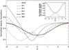Fig. 1 Large panel: normalized amplitudes of velocity fluctuations as a function of ξ = x/L for waves incident on the right side of a core with the density profile given by Eq. (35) for various values of the nondimensional wave frequency W. No dissipation is included. The dashed red line shows the WKB solution. Small panel: the red line shows the normalized density profile, and the black line the normalized Alfvén speed.

6. Application to molecular cloud cores

We applied our numerical schemes to the study of the propagation and damping of Alfvén waves in molecular cloud cores. We considered a one-dimensional cloud consisting of a low-mass core embedded in a uniform density envelope. For the cloud’s density we assumed a modified isothermal profile, $\mathit{\rho }\mathrm{=}\mathit{\mu }{\mathit{m}}_{\mathrm{H}}\mathrm{[}{\mathit{n}}_{\mathrm{env}}\mathrm{+}\mathrm{(}{\mathit{n}}_{\mathrm{core}}\mathrm{-}{\mathit{n}}_{\mathrm{env}}\mathrm{\left)}{\mathrm{sech}}^{\mathrm{2}}\mathrm{\right(}\mathit{\xi }{\mathrm{\left)}}^{\mathrm{\right]}}\mathit{,}$(35)with μ = 2.36, n_env = 10⁴ cm^-3, n_core = 10⁵ cm^-3, and ξ = x/L where L = 0.04 pc. The slab is threaded by a perpendicular, straight and uniform magnetic field of strength 70 μG and we considered the low-ionization regime typical of molecular cloud, ρ ≈ ρ_n. We assumed a simple ionization law, ${\mathit{\rho }}_{\mathrm{i}}\mathrm{=}\mathit{C}{\mathit{\rho }}^{\mathit{\kappa }}\mathit{,}$(36)with κ = 1/2 and C = 4.5 × 10^-17 cm^−3/2 g^1/2. With these values, and γ_in = 2.38 × 10¹⁴ cm³ g^-1 s^-1 (Pinto & Galli 2008), the ambipolar diffusion resistivity is ${\mathit{\eta }}_{\mathrm{AD}}\mathrm{=}\mathrm{3}\mathrm{\times }{\mathrm{10}}^{\mathrm{20}}{\left(\frac{\mathit{B}}{\mathrm{100} \mathit{\mu }\mathrm{G}}\right)}^{\mathrm{2}}{\left(\frac{\mathit{n}}{{\mathrm{10}}^{\mathrm{5}} {\mathrm{cm}}^{-3}}\right)}^{\mathrm{-}\mathrm{3}\mathit{/}\mathrm{2}} \mathrm{cm}\mathrm{2} {\mathrm{s}}^{-1}\mathit{.}$(37)The effect of wave reflection is illustrated in the following example, which describes the dependence of the velocity fluctuations on the normalized wave frequency W. We neglected dissipation (assuming η_AD = 0 and ℓ _⊥  = ∞) and assumed that only one outward propagating wave (z ₊ ) is injected at the right boundary. Solutions are obtained integrating backward from ξ = 3 and do not depend on the phase of the injected wave. The resulting velocity amplitudes are shown in Fig. 1 (large panel) for different values of the nondimensional frequency W ∈  [0.6,6] . Clearly, for increasing frequency the solution approaches the WKB analytical solution and the highest frequency case W = 6 is indistinguishable from it. The amplitude profiles show variations on a scale 1/k = V_A/ω that changes according to the Alfvén speed profile (shown in the small panel of Fig. 1), being smaller in the denser region  | ξ |  ≲ 1. This means that small scales are naturally formed in the core region.

The inclusion of diffusive effects requires a careful treatment of the boundary conditions. The choice of a symmetric density profile, with vanishing derivative at the cloud’s center and at infinity, allows one to match the asymptotic solutions with linear combinations of the solutions obtained by retaining only the terms that involve ambipolar diffusion (see Sect. 5.1), which we require to be exponentially damped waves. In practice, we assumed that at x = ∞ (x =  −∞) only leftward (rightward) propagating waves are present. The integration was carried out only in one half of the domain and we looked for solutions symmetric with respect to the core’s midplane. Since the gradients vanish at x = 0, the coupling given by reflection is absent and we can impose as boundary condition  | z₊(0) |  =  | z₋(0) |  there. We also averaged over eight phase differences (Δφ = nπ/4 with n = 0,1,...,7) between z₊(0) and z₋(0) to mimic the effect of incoherent wave sources at infinity. Results are shown in Fig. 2 for the range of normalized frequencies 0.6 < W < 6, and over a spatial interval corresponding to roughly three times the core size. The amplitudes of the waves were normalized to the values in ξ = 0. The frequency interval explored corresponds approximately to the wavelength interval L ≤ λ ≤ 10L in the core. In the high-frequency regime (W = 6), the damping length is comparable to the scale of the density gradient (x_d = 1.4 at ξ = 0), and the dominant effect is the quasi-exponential damping of the waves on a scale  ~ x_d. On the other hand, in the low-frequency regime (W = 0.6) the evolution of the wave amplitude is dominated by the the density gradient on a scale ξ ~ 1, because the damping length is much longer than the core’s size (x_d = 140 at ξ = 0).

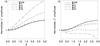Fig. 2 Normalized amplitudes of z −  (left panel ) and z +  (right panel ) as a function of ξ = x/L in a cloud core with the density profile given by Eq. (35) for values of the nondimensional wave frequency from W = 0.6 to W = 6.

Figure 3 shows the corresponding profiles of velocity fluctuations for the same range of frequencies as in Fig. 2. Again an average procedure was performed to take into account relative phases of uncorrelated waves moving in opposite directions from distant sources. As in the case of the amplitude of the Elsässer variables, the velocity amplitudes are mostly sensitive to the density gradient at lower frequencies W ~ 0.6 and mostly sensitive to the ambipolar damping at the highest frequencies (W ~ 6). This is easy to understand given the dependence of the ambipolar damping length on the inverse square of the frequency (Eq. (30)). Despite the simplicity and idealization of the model, it is clear that the sharp gradients of velocity dispersion observed in the environments of dense cores (Barranco & Goodman 1998; Caselli et al. 2002; Pineda et al. 2010) cannot be produced by a density gradient alone, but require the combined effects of a density gradient and ambipolar diffusion. In particular, sharp gradients in velocity amplitude are only possible when x_d ≈ 1, which implies waves with a frequency such as to give ℓ_d ≈ L. These waves have wavelength λ ~ (λ_crL)^1/2, intermediate between the critical wavelength λ_cr and the typical scale of the density gradient L.

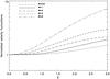Fig. 3 Normalized amplitude of velocity fluctuations as a function of ξ = x/L in a cloud core with the density profile given by Eq. (35) for values of the nondimensional wave frequency from W = 0.6 to W = 6.

6.1. Heating rate

The energy generated by the friction between streaming particles is a significant source of heating for molecular clouds (Scalo 1977; Lizano & Shu 1987). The energy produced heats the bulk of the gas, increasing its pressure and allowing chemical reactions to proceed at a faster rate (Flower et al. 1985; Pineau des Forêts et al. 1992). Therefore, it is important to evaluate the heating rate associated to the dissipation of the waves considered in the previous sections.

In a weakly ionized medium, the rate of energy generation by ambipolar diffusion (per unit time and unit volume) is $\mathit{H}\mathrm{=}\frac{\mathrm{|}{B}\mathrm{\times }\mathrm{(}\mathrm{\nabla }\mathrm{\times }{B}\mathrm{)}{\mathrm{|}}^{\mathrm{2}}}{\mathrm{16}{\mathit{\pi }}^{\mathrm{2}}{\mathit{\gamma }}_{\mathrm{in}}{\mathit{\rho }}_{\mathrm{i}}{\mathit{\rho }}_{\mathrm{n}}}$(38)(Braginskii 1965; see also Pinto et al. 2008). In the special case of low-amplitude Alfvén waves propagating in a one-dimensional medium, Eq. (38) reduces to $\mathrm{⟨}\mathit{H}\mathrm{⟩}\mathrm{=}\frac{{\mathit{\eta }}_{\mathrm{AD}}}{\mathrm{8}\mathit{\pi }}\mathrm{|}{b}\mathrm{\prime }{\mathrm{|}}^{\mathrm{2}}\mathit{,}$(39)where the brackets indicate the average over time and the prime a space derivative.

The heating rate as a function of position for waves propagating in the density profile given by Eq. (35) is shown in Fig. 4, as before for waves in the frequency range 0.6 ≤ W ≤ 6. To show the results in physical units, we have assumed b = B. Therefore, the values shown in the figure should be considered as upper limits to the actual value of the heating rate. For comparison, the red curve shows the cosmic-ray heating rate computed assuming a cosmic-ray ionization rate 3 × 10^-17 s^-1 and a mean energy deposited per ionization ΔQ = 20 eV (Goldsmith 2001). The ambipolar diffusion heating is clearly important both in the core and in the envelope, and competes with cosmic rays as a heating source for the cloud, especially for the highest values of the frequency. The behavior of the heating rate deviates significantly from the profile obtained assuming b′ ~ kb (see, e.g., Hennebelle & Inutsuka 2006), because of the modulation of the wave amplitude by the density gradient, and the space dependence of the damping length.

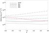Fig. 4 Ambipolar diffusion heating as a function of the normalized distance from the core center. For comparison, the red line shows the cosmic-ray heating rate for a cosmic-ray ionization rate 3 × 10-17 s-1 and energy deposition ΔQ = 20 eV.

6.2. Energy dissipation by turbulent cascade

In the previous section we have considered the dissipation of linear Alfvén waves caused by ion-neutral collisions. Here we estimate the effect of turbulent dissipation as given by the phenomenological expression (26). We decided to switch off ambipolar diffusion to better explore the effect of turbulence, varying its strength through the control parameter τ_A/τ_NL. Setting η_AD = 0 we set λ_cr = 0 and we did not have to worry about the first inequality in Eq. (24). We imposed at both sides of the cloud incoming fluctuations characterized by a frequency spectrum of width 1/t_A and then falling as ω^-2: energy is at long wavelengths and ℓ_|| ≈ V_A0t_A = L. We here discuss four runs in which we varied the turbulent strength τ_A/τ_NL by changing the input amplitude and perpendicular scale as listed in Table 1. The strong turbulence cases are runs A and D, the last even though it has a smaller input amplitude. The time-averaged, turbulent heating rate per unit volume follows directly from Eq. (26) and is given by ${\mathit{H}}_{\mathrm{T}}\mathrm{=}{\mathit{\rho }}_{\mathrm{n}}\frac{\mathrm{\left|}{\mathit{z}}_{\mathrm{-}}\mathrm{\right|}\mathrm{|}{\mathit{z}}_{\mathrm{+}}{\mathrm{|}}^{\mathrm{2}}\mathrm{+}\mathrm{|}{\mathit{z}}_{\mathrm{+}}\mathrm{\left|}\mathrm{\right|}{\mathit{z}}_{\mathrm{-}}{\mathrm{|}}^{\mathrm{2}}}{\mathrm{2}{\mathit{\ell }}_{\mathrm{\perp }}}\mathrm{\propto }{\mathit{\rho }}_{\mathrm{n}}\mathit{f}\mathrm{\left(}{\mathit{\sigma }}_{\mathrm{c}}\mathrm{\right)}\frac{{\mathit{E}}^{\mathrm{3}\mathit{/}\mathrm{2}}}{\mathrm{2}{\mathit{\ell }}_{\mathrm{\perp }}}\mathit{,}$(40)where ${\mathit{\sigma }}_{\mathrm{c}}\mathrm{=}\frac{\mathrm{|}{\mathit{z}}_{\mathrm{+}}{\mathrm{|}}^{\mathrm{2}}\mathrm{-}\mathrm{|}{\mathit{z}}_{\mathrm{-}}{\mathrm{|}}^{\mathrm{2}}}{\mathrm{|}{\mathit{z}}_{\mathrm{+}}{\mathrm{|}}^{\mathrm{2}}\mathrm{+}\mathrm{|}{\mathit{z}}_{\mathrm{-}}{\mathrm{|}}^{\mathrm{2}}}$(41)is the (normalized) cross helicity, E =  | z ₊  | ² +  | z ₋  | ² is the total turbulent energy, and $\mathit{f}\mathrm{\left(}{\mathit{\sigma }}_{\mathrm{c}}\mathrm{\right)}\mathrm{=}\sqrt{\mathrm{1}\mathrm{-}{\mathit{\sigma }}_{\mathrm{c}}^{\mathrm{2}}}\mathrm{(}\sqrt{\mathrm{1}\mathrm{+}{\mathit{\sigma }}_{\mathrm{c}}}\mathrm{+}\sqrt{\mathrm{1}\mathrm{-}{\mathit{\sigma }}_{\mathrm{c}}}\mathrm{)}$ is a symmetric function that vanishes at  | σ_c |  = 1 and increases monotonically, reaching a maximum f(0) = 1.

The small amount of energy at high frequency justifies neglecting ambipolar diffusion, we verified that  ⟨ H ⟩  ≪ H_T for $\begin{array}{}{}_{\mathrm{˜}}\\ {\mathit{\eta }}_{\mathrm{AD}}\end{array}\mathrm{\simeq }{\mathit{\lambda }}_{\mathrm{cr}}\mathit{/}{\mathit{\ell }}_{\mathrm{\left|}\mathrm{\right|}}\lesssim \min \mathrm{(}\mathit{b}\mathit{/}\mathit{B}\mathrm{)}\mathrm{=}\mathrm{0.1}$.

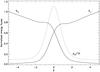Fig. 5 Time-averaged normalized energy fluxes entering the cloud from both sides, S+/S+(ξ =  −5) and S−/S−(ξ = 5), for run B. The normalized density profile is shown for comparison by the dotted line.

Let us examine the case of intermediate turbulence strength, ${\mathit{\tau }}_{\mathrm{A}}\mathit{/}{\mathit{\tau }}_{\mathrm{NL}}\mathrm{=}\mathrm{1}\mathit{/}\sqrt{\mathrm{10}}$ (run B). In the linear case with η_AD = 0, the coupling between z_± in proximity of the density gradients causes an enhancement of the respective energy fluxes S _± , which have a bump toward the cloud’s center. This ensures the conservation of the net energy flux (S₊ − S₋), which is uniform. When nonlinear dissipation is taken into account, the profiles of S₊ and S₋ are remarkably different, as shown in Fig. 5 where we also plot the density profile for comparison (dotted line). Both energy fluxes decrease toward the cloud’s center, indicating the damping of the wave (heating). In contrast to the linear case, there is a sharp decrease on the core size due to the turbulent heating H_T, which is stronger in the whole core (being approximately proportional to ρ_n). From Fig. 5 one can also deduce the behavior of σ_c, which is also equal to (S ₊  − S ₋ )/(S ₊  + S ₋ ) (the fluxes are normalized to their respective incident value, since S ₊ (ξ =  −5) ≈ S ₋ (ξ = 5) the normalization factors can be considered equal). The normalized cross helicity vanishes at the core’s center and increases rapidly in the core’s envelope, maintaing a value  | σ_c |  ≳ 0.8 at the edges of the core. The cross helicity and the total turbulent energy affect the average heating rate per unit mass (H_T/ρ_n), which is plotted in Fig. 6 for the four runs (run B corresponding to the dashed line). For weak turbulence (runs B and C) the profile is basically flat, varying by 20% at maximum, and thus reflecting H_T ∝ ρ_n. Interestingly, it is flat on a region entirely surrounding the core and peaks outside it, showing that the wave damping is maximal when passing from the cloud to the core. The relatively flat profile can be explained in terms of a compensation of the terms related to the cross-helicity and total turbulent energy in Eq. (40). Indeed, the cascade is more balanced (σ_c ≈ 0) at the center, but less energetic, while the turbulent energy grows outside the core, but the cascade is less balanced. For stronger turbulence (e.g. τ_A/τ_NL = 1) these two effects do not compensate each other anymore and the minima and maxima in the heating rate are more pronounced (H_T follows the scaling with ρ_n less closely). Note that keeping τ_A/τ_NL = 1 but varying the input amplitudes b/B = ℓ _⊥ /ℓ _|  |  = 1/10 the profile does not vary, but the overall dissipation decreases (compare runs A and D). One can verify that the average dissipation per unit mass scales as ${\mathit{H}}_{\mathrm{T}}\mathit{/}{\mathit{\rho }}_{\mathrm{n}}\mathrm{\propto }\mathrm{1}\mathit{/}{\mathit{\tau }}_{\mathrm{NL}}^{\mathrm{2}}$, while the relative excursion at the core edges ΔH_T/H_T grows with τ_NL/τ_A.

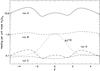Fig. 6 Profile of the time-averaged heating rate per unit mass (in nondimensional units) for different turbulent strength τA/τNL = 1, 1/$\sqrt{\mathrm{10}}\mathit{,} \mathrm{1}\mathit{/}\mathrm{10}\mathit{,} \mathrm{1}$, corresponding to runs A, B, C, D as labeled on each curve (solid, dashed, dot-dashed and long-dashed lines, respectively). The normalized density profile is shown for comparison as a dotted line.

7. Conclusions

We have considered the propagation of Alfvén waves in a density profile typical of a molecular cloud core embedded in a low-density medium. The formulation of the problem in terms of Elsässer variables was found particularly appropriate to treat the effects of wave reflection and dissipation. We have studied with time-dependent as well as time-independent numerical codes the interaction of incoherent wave trains incident on the opposite edges of a one-dimensional model cloud, determining the amplitude variations associated to the reflection and damping of the waves.

We found that for waves with a wavelength longer than the critical wavelength, of the order of a few 10^-3 pc in a molecular cloud core, but shorter or of the order of the size of the core, a significant decrease in the velocity amplitude is produced by the combined effects of reflection at the core’s boundaries and dissipation due to ambipolar diffusion in the core’s interior. For these waves, the damping length associated to ion-neutral collisions is of the same order as the size of the core. The resulting behavior of the amplitude of velocity fluctuations may explain, at least in part, the sharp decrease of line widths observed in the environments of low-mass cores (see Sect. 1). Moreover, for these waves the energy generated by ion-neutral drift is a significant source of heating both in the core and its envelope (see Sect. 6.1).

We also considered the turbulent dissipation and found that the average heating per unit mass scales as 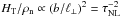${\mathit{H}}_{\mathrm{T}}\mathit{/}{\mathit{\rho }}_{\mathrm{n}}\mathrm{\propto }\mathrm{(}\mathit{b}\mathit{/}{\mathit{\ell }}_{\mathrm{\perp }}{\mathrm{)}}^{\mathrm{2}}\mathrm{=}{\mathit{\tau }}_{\mathrm{NL}}^{-2}$, thus becoming significant for high enough wave amplitudes (0.1 < b/B < 1). This regime is particularly relevant for molecular clouds and star-forming regions where a statistical analysis of dust polarization maps suggests that the ratio of the strength of turbulent magnetic field to the large-scale mean field is of the order of 0.1–0.5 (Hildebrand et al. 2009; Houde et al. 2009). We used a phenomenological term to mimic the effect of a perpendicular turbulent cascade. The results of our calculations show that the turbulent cascade affects the amplitude of fluctuations both at the cloud’s edge and in the cloud’s interior. In particular, the energy dissipation (per unit mass) associated to this process is peaked in the regions immediately surrounding the dense central core, indicating a stronger damping of the wave amplitude. The relative excursion between maxima and minima ΔH_T/H_t depends on the turbulence strength τ_NL/τ_A, so it can be significant even for small amplitudes, provided the turbulent correlation length is of the order of a few times the size of the core. In a more realistic situation, the turbulent cascade, although it is stronger in the perpendicular direction, also generates small parallel scales. Therefore we expect that turbulence and ambipolar diffusion will be at work at the same time, enhancing the sharp variation of velocity amplitude at the interface between the cloud and the core. In the present work the investigation of the parameter space was limited by the several assumptions (Eq. (24)) we made to obtain the model equations. Interesting features appear when we are close to the limit of the allowed parameter space. Additional work is needed to address these issues with a more realistic and detailed modeling of turbulence that includes the effects of ambipolar diffusion.

Acknowledgments

We would like to thank Stella Galligani for carrying out some of the nonlinear simulations with the phenomenological model of turbulence.

References

All Tables

All Figures

Fig. 1 Large panel: normalized amplitudes of velocity fluctuations as a function of ξ = x/L for waves incident on the right side of a core with the density profile given by Eq. (35) for various values of the nondimensional wave frequency W. No dissipation is included. The dashed red line shows the WKB solution. Small panel: the red line shows the normalized density profile, and the black line the normalized Alfvén speed.

In the text

	Fig. 2 Normalized amplitudes of z −  (left panel ) and z +  (right panel ) as a function of ξ = x/L in a cloud core with the density profile given by Eq. (35) for values of the nondimensional wave frequency from W = 0.6 to W = 6.
In the text

	Fig. 3 Normalized amplitude of velocity fluctuations as a function of ξ = x/L in a cloud core with the density profile given by Eq. (35) for values of the nondimensional wave frequency from W = 0.6 to W = 6.
In the text

	Fig. 4 Ambipolar diffusion heating as a function of the normalized distance from the core center. For comparison, the red line shows the cosmic-ray heating rate for a cosmic-ray ionization rate 3 × 10-17 s-1 and energy deposition ΔQ = 20 eV.
In the text

	Fig. 5 Time-averaged normalized energy fluxes entering the cloud from both sides, S+/S+(ξ =  −5) and S−/S−(ξ = 5), for run B. The normalized density profile is shown for comparison by the dotted line.
In the text

Fig. 6 Profile of the time-averaged heating rate per unit mass (in nondimensional units) for different turbulent strength τA/τNL = 1, 1/$\sqrt{\mathrm{10}}\mathit{,} \mathrm{1}\mathit{/}\mathrm{10}\mathit{,} \mathrm{1}$, corresponding to runs A, B, C, D as labeled on each curve (solid, dashed, dot-dashed and long-dashed lines, respectively). The normalized density profile is shown for comparison as a dotted line.

In the text

References

- Arons, J., & Max, C. E. 1975, ApJ, 196, L 77 [Google Scholar]
- Barranco, J. A., & Goodman, A. A. 1998, ApJ, 504, 207 [NASA ADS] [CrossRef] [Google Scholar]
- Braginskii, S. 1965, in Rev. Plasma Physics, ed. M. Leontovich (New York: Consultants Bureau), 1, 205 [Google Scholar]
- Campos, L. M. B. C., & Isaeva, N. L. 1993, Adv. Space Res., 13, 123 [NASA ADS] [CrossRef] [Google Scholar]
- Caselli, P., Benson, P. J., Myers, P. C., & Tafalla, M. 2002, ApJ, 572, 238 [NASA ADS] [CrossRef] [Google Scholar]
- Coker, R. F., Rae, J. G. L., & Hartquist, T. W. 2000, A&A, 360, 290 [NASA ADS] [Google Scholar]
- Dobrowolny, M., Mangeney, A., & Veltri, P. 1980, Phys. Rev. Lett., 45, 144 [NASA ADS] [CrossRef] [Google Scholar]
- Dmitruk, P., Milano, L. J., & Matthaeus, W. H. 2001, ApJ, 548, 482 [NASA ADS] [CrossRef] [Google Scholar]
- Elsässer, W. M. 1950, Phys. Rev., 79, 153 [Google Scholar]
- Flower, D. R., Pineau des Forêts, G., & Hartquist, T. W. 1985, MNRAS, 216, 775 [NASA ADS] [CrossRef] [Google Scholar]
- Galtier, S., Nazarenko, S. V., & Newell, A. C. 2002, ApJ, 564, 49 [Google Scholar]
- Goldreich, P., & Sridhar, S. 1995, ApJ, 438, 763 [NASA ADS] [CrossRef] [Google Scholar]
- Goldsmith, P. F. 2001, ApJ, 557, 763 [Google Scholar]
- Goodman, A. A., Barranco, J. A., Wilner, D. J., & Heyer, M. H. 1998, ApJ, 504, 223 [NASA ADS] [CrossRef] [Google Scholar]
- Hennebelle, P., & Inutsuka, S.-I. 2006, ApJ, 647, 404 [NASA ADS] [CrossRef] [Google Scholar]
- Heitsch, F., & Burkert, A. 2002, in Modes of Star Formation and the Origin of Field Populations, eds. E. K. Grebel, & W. Brandner, ASP Conf. Ser., 285, 13 [Google Scholar]
- Hildebrand, R. H., Kirby, L., Dotson, J. L., Houde, M., & Vaillancourt, J. E. 2009, ApJ, 696, 567 [NASA ADS] [CrossRef] [Google Scholar]
- Hollweg, J. V. 1981, Sol. Phys., 70, 25 [NASA ADS] [CrossRef] [Google Scholar]
- Houde, M., Vaillancourt, J. E., Hildebrand, R. H., Chitsazzadeh, S., & Kirby, L. 2009, ApJ, 706, 1504 [NASA ADS] [CrossRef] [Google Scholar]
- Kudoh, T., & Basu, S. 2003, ApJ, 595, 842 [NASA ADS] [CrossRef] [Google Scholar]
- Kudoh, T., & Basu, S. 2006, ApJ, 642, 270 [NASA ADS] [CrossRef] [Google Scholar]
- Kulsrud, R., & Pearce, W. P. 1969, ApJ, 156, 445 [Google Scholar]
- Lizano, S., & Shu, F. H. 1987, in Physical Processes in Interstellar Clouds, NATO ASIC Proc., 210, 173 [Google Scholar]
- Mac Low, M.-M. 1999, ApJ, 169, 178 [Google Scholar]
- Malara, F., & Velli, M. 1996, J. Geophys. Res., 92, 7363 [Google Scholar]
- Marsch, E., & Mangeney, A. 1987, Phys. Plasmas, 3, 4427 [Google Scholar]
- Martin, C. E., Heyvaerts, J., & Priest, E. R. 1997, A&A, 326, 1176 [NASA ADS] [Google Scholar]
- Myers, P. C., & Khersonsky, V. K. 1995, ApJ, 442, 186 [NASA ADS] [CrossRef] [Google Scholar]
- Nakano, T., Nishi, R., & Umebayashi, T. 2002, ApJ, 573, 199 [NASA ADS] [CrossRef] [Google Scholar]
- Ormel, C. W., Paszun, D., Dominik, C., & Tielens, A. G. G. M. 2009, A&A, 502, 845 [NASA ADS] [CrossRef] [EDP Sciences] [Google Scholar]
- Oughton, S., Dmitruk, P., & Matthaeus, W. H. 2004, Phys. Plasmas, 11, 2214 [NASA ADS] [CrossRef] [Google Scholar]
- Pandey, B. P., Vladimirov, S. V., & Samarian, A. 2008, Phys. Plasmas, 15, 053705 [NASA ADS] [CrossRef] [Google Scholar]
- Piddington, J. H. 1956, MNRAS, 116, 314. [NASA ADS] [CrossRef] [Google Scholar]
- Pineda, J. E., Goodman, A. A., Arce, H. G., et al. 2010, ApJ, 712, L116 [NASA ADS] [CrossRef] [Google Scholar]
- Pineau des Forêts, G., Roueff, E., & Flower, D. R. 1992, MNRAS, 258, 45 [NASA ADS] [CrossRef] [Google Scholar]
- Pinto, C., & Galli, D. 2008, A&A, 484, 17 [NASA ADS] [CrossRef] [EDP Sciences] [Google Scholar]
- Pinto, C., Galli, D., & Bacciotti, F. 2008, A&A, 484, 1 [NASA ADS] [CrossRef] [EDP Sciences] [Google Scholar]
- Scalo, J. M. 1977, ApJ, 213, 705 [NASA ADS] [CrossRef] [Google Scholar]
- Shebalin, J. V., Matthaeus, W. H., & Montgomery, D. 1983, J. Plasma Phys., 29, 525 [NASA ADS] [CrossRef] [Google Scholar]
- Tang, Y.-W., Ho, P. T. P., Koch, P. M., et al. 2009, ApJ, 700, 251 [NASA ADS] [CrossRef] [Google Scholar]
- Velli, M. 1993, A&A, 270, 304 [NASA ADS] [Google Scholar]
- Verdini, A., Velli, M., Matthaeus, W.H., et al. 2010, ApJ, 708, 116 [Google Scholar]
- von Kármán, T., & Howarth, L. 1938, Proc. Roy. Soc. London Ser. A, 164, 192 [Google Scholar]
- Walén, C. 1944, Arkiv. Mat. Astr. Fys., 30A, 15 [Google Scholar]
- Wardle, M., & Ng, C. 1999, MNRAS, 303, 239 [NASA ADS] [CrossRef] [Google Scholar]
- Zweibel, E. G., & Josafatsson, K. 1983, ApJ, 270, 511 [CrossRef] [Google Scholar]
All Tables
Nondimensional parameters for the runs: input amplitude (b/B) and ratio of the perpendicular to parallel scales of fluctuations (ℓ⊥/ℓ||).