| Issue |
A&A
Volume 544, August 2012
|
|
|---|---|---|
| Article Number | A151 | |
| Number of page(s) | 11 | |
| Section | Astrophysical processes | |
| DOI | https://doi.org/10.1051/0004-6361/201218921 | |
| Published online | 21 August 2012 | |
Magnetic field induced by strong transverse plasmons in ultra-relativistic electron-positron plasmas
1 School of Sciences, Nantong University, 226019 Nantong, PR China
e-mail: This email address is being protected from spambots. You need JavaScript enabled to view it.
2 Department of Physics, Nanjing Normal University, 210097 Nanjing, PR China
3 School of Sciences, Nanchang University, 330047 Nanchang, PR China
Received: 31 January 2012
Accepted: 4 July 2012
Abstract
Context. We investigated the generation of localized magnetic fields in an ultra-relativistic non-isothermal electron-positron plasma by strong electromagnetic plasmons.
Aims. The results obtained can be used to explain the origin of small-scale magnetic fields in the internal shock region of gamma-ray bursts with ultra-relativistic electron positron plasmas.
Methods. The generation of magnetic fields was investigated with kinetic Vlasov Maxwell equations.
Results. The self-generated magnetic field will collapse for modulation instability, leading to spatially highly intermittent magnetic fluxes, whose characteristic scale is much larger than relativistic plasma skin depth, which in turn is conducive to the generation of the long-life small-scale magnetic fields in the internal shock region of gamma-ray bursts.
Key words: gamma-ray burst: general / magnetic fields / relativistic processes / plasmas
© ESO, 2012
1. Introduction
The prompt emission and afterglows of gamma-ray bursts (GRBs) are generally believed to be produced by synchrotron emission. Although the synchrotron emission can adequately explain the observed afterglow spectra and light curves, yet there are some problems in fitting the observed prompt γ-ray spectrum. On the one hand, the theoretically predicted spectrum in the low-energy part of the synchrotron spectrum contradicts the much harder spectra observed. Considering the fast cooling of electrons by synchrotron emission (Cohen et al. 1997), this problem will be even more severe. On the other hand, many observational spectra showed turnoff points and energy excesses in the higher frequency parts. These problems may be caused by a significant decrease of the synchrotron emission mechanism in which the magnetic field should be uniform throughout the shocked region.
Medvedev (2000) proposed that the prompt emission is produced by jitter radiation, which arises if the magnetic field’s correlation length is smaller than the region over which an electron emits the synchrotron radiation seen by a given observer. This radiative mechanism has been applied successfully to the research of gamma-ray bursts (Medvedev 2006; Mao & Wang 2011) and their afterglows (Workman et al. 2008; Morsony et al. 2009). To overcome that the electron cooling time is much shorter than the dynamical time (Ghisellini et al. 2000), Pe’er & Zhang (2006) put forward that the magnetic field created by the internal shocks decays on a length scale much shorter than the comoving width of the plasma. Under this assumption synchrotron radiation can reproduce the observed prompt emission spectra of the majority of the bursts. Deng et al. (2005) applied the synchro-curvature mechanism instead of the synchrotron mechanism to explain the spectra of gamma-ray bursts. They demonstrated that if the curvature radius of magnetic fields is much smaller than the scale of the emission area, many observational spectra with turnoff points and energy excesses in the higher frequency parts can be fit nicely. These theories indicate the turbulent small-scale magnetic field is crucial for our understanding of GRBs.
Medvedev & Loeb (1999) suggested that the relativistic Weibel instability can generate strong small-scale magnetic fields in the collisionless shocks of GRBs. However, Gruzinov (2001) raised the concern that this magnetic field will maintain its equipartition magnitude only over a skin depth δ, they decay there on a timescale  due to phase-space mixing, but generic synchrotron emission scenarios take place on longer timescales, ranging from 105 to
  . Magnetic field decay may be alleviated via an inverse cascade from small to large scales. An inverse cascade via current filament merging operates strongly in the foreshock region (Silva et al. 2003). However, Katz et al. (2007) suggested via self-similar arguments that the inverse cascade does not operate downstream of the shock. Chang et al. (2008) investigated the idea by two-dimensional particle-in-cell numerical simulations. These authors found that filament merging does occur, but is confined to the foreshock, where the filaments exist, and there is little evidence of magnetic clumps merging in the downstream. Hence, the magnetic energy should evaporate in the downstream region. Therefore, Chang and collaborators concluded that initially unmagnetized relativistic shocks in electron-positron plasmas are unable to form persistent downstream magnetic fields, if there are no additional physical processes that create longer wavelength, more persistent fields. In this paper we investigate the generation of magnetic fields in the relativistic EP plasma from a different perspective.
Pulupa et al. (2010) examined 178 interplanetary shocks observed by the Wind spacecraft. They found 43 produced upstream Langmuir waves, as that shown by enhancements in wave power near the plasma frequency. In the foreshock region, the reflected electron beams create unstable bump-on-tail electron distribution functions, which excite a Landau resonance and create electrostatic oscillations known as Langmuir waves. Medvedev & Loeb (1999) also pointed out that if the colliding shells do not possess similar densities, the growth rate of the instability decreases or even shuts off beyond a particular density contrast. In this regime, the shock may be dominated by electrostatic (Langmuir) turbulence. The Langmuir waves undergo a mode conversion process and generate electromagnetic waves at the plasma frequency. There is a continuous transfer from Langmuir waves to transverse plasmons and back, and their energy densities are approximately the same, average over time, Wl ≈ WT (Kaplan & Tsytovich 1973; Liu et al. 2008).
The prompt γ-rays in the GRBs are assumed to be produced by internal shock that may be dominated by the ultra-relativistic electron-positron pairs (Medvedev et al. 2005). In our previous paper we have come to the conclusion that the interaction of transverse plasmons with isothermal ultra-relativistic EP plasma will not excite magnetic field (Liu & Liu 2011). The reason is that the same mass and the opposite charge of EP pairs leads to the cancellation of magnetic currents, while one can expect that the spontaneous magnetic field maybe present for non-isothermal ultra-relativistic EP plasma, i.e., Te ≠ Tp. Tkaczyk (1993) used a non-isothermal EP plasma model to explain the observed spectra of gamma ray bursts. He suggested that the relaxation time may exceed the annihilation time when temperature of electron and positron are significantly different, and argued that in the emission region of the gamma burst source the temperature of electrons and positrons can be different because of, i) the additional heating mechanism of the electrons or the positrons is in action; or, ii) turbulent motion causes the injection of the hot plasma to the cool region; or, iii) a strong magnetic field. For the sake of simplicity, we assume that electron thermal temperature is much higher than that of positrons, i.e., Te ≫ Tp (Karpman et al. 1975). The dispersion relation for an electromagnetic wave with frequency close to ωP in the plasma is (Mikhailovskii 1980)  (1)in which
  ,
,  is the positron (or electron) plasma frequency; ap,e = mec2/Tp,e, for ultra-relativistic case ap,e ≪ 1; n0, me, e and Tp,e are the particle density for electrons and positrons in equilibrium state, the electron rest mass, the electron charge magnitude, and the thermal temperature of positrons and electrons, respectively. This wave is undamped in a collisionless unmagnetized plasma because its phase velocity always exceeds the speed of light. Hence, they cannot resonate with plasma particles. It is extremely difficult for the oscillations to escape the plasma because the refraction index of the wave is very close to zero. This means that once the mode is excited, it will stay at the source region where there are strong nonlinear wave-wave and wave-particle interactions. It is convenient to call the transverse mode of Eq. (1) transverse plasmon. In the following, we will theoretically investigate the low-frequency magnetic filed generated by the transverse electromagnetic plasmons with dispersion (1). Qualitatively understanding the excitation of magnetic fields by transverse plasmons is quite straightforward: low-frequency nonlinear currents excited by high-frequency transverse plasmons via wave-wave and wave-particle interactions lead to the generation of quasi-static magnetic field.
An important property that distinguishes high-temperature relativistic plasmas from normal fluids is that the plasmas are to a first approximation collisionless (O’Neil & Coroniti 1999). In view of this fact, the governing equations for the magnetic field generated in the interactions of transverse plasmons with ultra-relativistic non-isothermal EP plasmas are derived from Vlasov-Maxwell equations, in which nonlinear wave-wave and wave-particle interactions are taken into consideration. The modulation instability of finite transverse plasmons shows that the characteristic scale of the spontaneous magnetic field is much larger than the relativistic plasma skin depth. Therefore, one can expect that the magnetic field will have a longer lifetime than the field generated by Weibel instability. Our theory may provide a new insight into the origin of magnetic fields in the internal shocks of GRBs.
2. Nonlinear governing equations for the interactions of transverse plasmons with non-isothermal ultra-relativistic EP plasmas
2.1. Fundamental theory in the framework of Vlasov-Maxwell equation
If the exited energy density of a perturbed field ET is much lower than the thermal one, i.e.,  (2)the perturbed distribution function of plasma particles can be expanded in powers of the field ET (Tsytovich 1977). In this case, taking the well-known kinetic Vlasov equation as well as the Maxwell equations into consideration, following the method introduced by Li & Ma (1993), one can obtain the equations for a transverse field
  (3)and for longitudinal field
 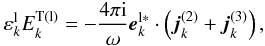 (4)where only the nonlinear currents up to the third order have been considered.
  is the second-order nonlinear current
 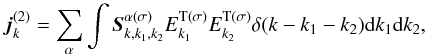 (5)the third-order nonlinear current
 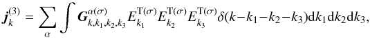 (6)with
 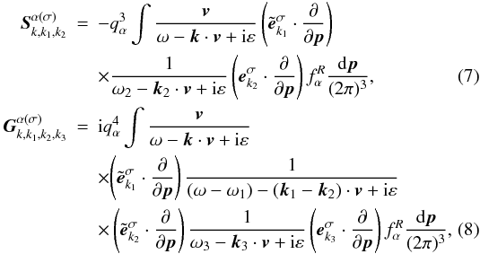 in which ∗ denotes the conjugate;
  and
and  are transverse and longitudinal dielectric constants; the term iε arises from the Landau rule (Lifshitz & Pitaevskii 1981);
  is unit polarization vector for σ-mode (for transverse mode, σ = t, and for longitudinal mode, σ = l);
  ,
,  . It is worth noting that under the high-frequency approximation, i.e, ω ≈ ωP ≫ kc, one derives
  . The δ functions in Eqs. (5) and (6) represent the conservation of energy and momentum.
  is the equilibrium distribution function of plasma particles. Liang (1982) had mentioned that even collisionless plasmas can maintain near-Maxwellian distributions via collective processes, thus, we may take the distribution function of particles in equilibrium unperturbed state to be (Jüttner 1911)
  (9)where
  is the usual Lorentz factor, K2 is the second kind modified Bessel function of the second order.
From Eqs. (7) and (8) one can see  ,
,  ,
,  . Considering the relativistic effects, one has
  . Since the distribution function (9) has an exponential form, the characteristic value of γα ~ 1/aα. When Te ≫ Tp, the characteristic value of γe is much higher than that of γp. Therefore, the nonlinear currents produced by the electrons can be neglected. That is to say, one can take α = p and omit the symbol ∑ in Eqs. (5) and (6).
2.2. Self-generated low-frequency magnetic fields
The low-frequency nonlinear current is generated by nonlinear interactions of two intense waves that propagate in opposite directions, leading to the the low-frequency transverse and longitudinal fields. Now, we study the low-frequency transverse field, i.e.,  in Eq. (3). Only considering the second order of
  , Eq. (3) gives (Li & Ma 1993)
 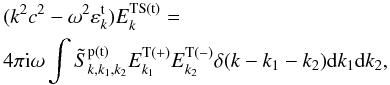 (10)in which + and – denote positive and negative high-frequency fields, k1 = (k1,ω1) and k2 = (k2,ω2) are four-dimensional wave vectors for positive and negative high-frequency transverse fields, k = (k,ω) is the four-dimensional wave vector for low-frequency transverse fields. The interaction matrix
 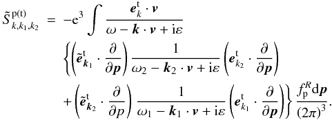 (11)Here and below we assume that all field quantities and their differentials satisfy the natural boundary condition, i.e., they are to be zero at infinity. Under the assumption of low-frequency fields kc ≪ ω ≪ ωP, of high-frequency fields ω1 ≈ − ω2 ≈ ωP, and the isotropic distribution of positrons, the interaction matrix Eq. (11) can be reduced to be (see Appendix A)
 ![Mathematical equation: \begin{equation} \label{eq12} \tilde {S}_{k,k_1 ,k_2 }^{\rm p\left( {t} \right)} \approx -\frac{1}{4\pi }\frac{e\omega _{\rm pp}^2 }{m_{\rm p} \omega \omega _{\rm P}^2 }\Lambda {{\vec e}}_{k}^{\rm t\ast } \cdot \left[ {{{\vec k}}\times \left( {{{\vec e}}_{{k}_1 }^{\rm t} \times {{\vec e}}_{{k}_2 }^{\rm t} } \right)} \right], \end{equation}](/articles/aa/full_html/2012/08/aa18921-12/aa18921-12-eq64.png) (12)where
(12)where 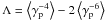 , in which,
  and
and 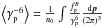 .
.
The transverse dielectric constants for ultra-relativistic positrons and electrons are  and
and  , for kc ≪ ω ≪ ωP, respectively (Mikhailovskii 1980). Correspondingly, one can arrive at
  . Here, we used the formula
  . Therefore, substituting Eqs. (12) into (11) yields
  (13)Timing both sides of Eq. (13) with k, and taking Faraday’s law into consideration, i.e.,
  , the equation for spontaneous low-frequency magnetic field in Fourier space can be obtained
  (14)From above equation, one can find that the self-generated magnetic field is exited by the nonlinear wave-wave coupling.
2.3. High-frequency transverse field
If  in the left-hand side of Eq. (3) is a positive high-frequency transverse field, i.e.,
  . The quadratic terms in Eq. (5) should be the product of high-frequency and low-frequency fields:
  . The three field products included in the current
  can be expressed in terms of the triple product of high-frequency fields and a mixed cubic product of high-frequency and low-frequency fields. Considering Eq. (11), this mixed term is indeed the product of four high-frequency fields, which is of higher order. Then,
 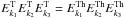 . Because the presence of the factor (ω − ω1) − (k1 − k2)·v + iε in the integral expression for
  is important when
  is the perturbed field with positive frequency. As a result,
 ![Mathematical equation: \hbox{$E_{k_1 }^{\rm T} E_{k_2 }^{\rm T} E_{k_3 }^{\rm T} = E_{k_1 }^{\rm T( + )} [E_{k_2 }^{\rm T( + )} E_{k_3 }^{\rm T( - )} + E_{k_2 }^{\rm T( - )} E_{k_3 }^{\rm T( + )} ]$}](/articles/aa/full_html/2012/08/aa18921-12/aa18921-12-eq85.png) . Now, we obtain the high-frequency field equation from Eq. (3) (Li & Ma 1993)
. Now, we obtain the high-frequency field equation from Eq. (3) (Li & Ma 1993) 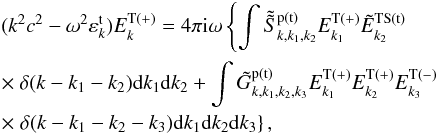 (15)in which the matrix element for two positive and one negative high-frequency transverse field coupling to positive high-frequency transverse field is
 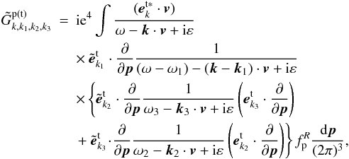 (16)and
  is the same as
  , except that k2 is the four-dimensional wave vector for the low-frequency transverse field. The low-frequency transverse field ETS(t) for the fusion process of Eq. (11) may be different from the low-frequency field
  for the decay process in Eq. (15). According to the semi-classical theory, the decay/fusion interactions can determine the intensity of the low-frequency field
  . In other words, they differ by a phase factor exp(iϕ):
  (Li & Ma 1993).
To obtain the high-frequency transverse field equation, one should estimate the nonlinear interaction matrixes and  in detail. Considering that ω1 ≈ ωP ≫ k1c and ω ≈ ωP ≫ kc for high-frequency transverse fields, k2c ≪ ω2 ≪ ωP and
  for the low-frequency transverse field, after straightforward manipulation, one can obtain (see Appendix B )
 ![Mathematical equation: \begin{equation} \label{eq17} \tilde {\tilde {S}}_{k,k_1 ,k_2 }^{\rm p\left( t \right)} \approx - \frac{1}{4\pi }\frac{\omega _{\rm pp}^2 e}{\omega m_{\rm p} \omega _{\rm P} c}\left\langle {\gamma _{\rm p}^{ - 4} } \right\rangle {\vec e}_{k}^{\rm t{\rm {\bf \ast }}} \cdot \left[ {{\vec e}_{{{k}}_1 }^{\rm t} \times \left( {\frac{{\vec k}_2 c}{\omega _2}\times {{\vec e}}_{{k}_2 }^{\rm t} } \right)} \right]. \end{equation}](/articles/aa/full_html/2012/08/aa18921-12/aa18921-12-eq101.png) (17)Integrating Eq. (16) by parts, and considering ω ≈ ωP ≫ kc, Eq. (16) can be written as
(17)Integrating Eq. (16) by parts, and considering ω ≈ ωP ≫ kc, Eq. (16) can be written as  (18)Regarding that the characteristic Lorentz factor for positrons γp ~ 1/ap, the above equation can be simplified to
  (19)where
 ![Mathematical equation: \begin{eqnarray} H_{k-k_{1},k_{2},k_{3}}^{\rm p} &=&-\frac{{\rm e}^{2}}{(\omega -\omega _{1})-({ {\vec k}}-{{\vec k}}_{1})\cdot {{\vec v}}+{\rm i}\varepsilon } \notag \\ &&\times\left[ {\tilde{{{\vec e}}}_{{k}_{2}}^{\rm t}\cdot \frac{\partial }{\partial {{\vec p}}}\frac{1}{\omega _{3}-{ {\vec k}}_{3}\cdot {{\vec v}}+{\rm i}\varepsilon }{{\vec e}}_{ {k}_{3}}^{\rm t}\cdot \frac{\partial }{\partial {{\vec p }}}}\right. \notag \\ &&\left. {+{\tilde{{\vec e}}}_{{k}_{3}}^{\rm t}\cdot \frac{\partial }{\partial {{\vec p}}}\frac{1}{\omega _{2}-{ {\vec k}}_{2}\cdot {{\vec v}}+{\rm i}\varepsilon }{{\vec e}}_{ {k}_{2}}^{\rm t}\cdot \frac{\partial }{\partial {{\vec p }}}}\right] f_{\rm p}^{R}. \label{eq20} \end{eqnarray}](/articles/aa/full_html/2012/08/aa18921-12/aa18921-12-eq105.png) (20)The second-order low-frequency density perturbation produced by the interaction of two high-frequency transverse fields propagating in opposite directions is (Li & Ma 1993)
(20)The second-order low-frequency density perturbation produced by the interaction of two high-frequency transverse fields propagating in opposite directions is (Li & Ma 1993)  (21)where
  is the same as
  , except k − k1 → k, k2 → k1, k3 → k2. Here we should mention that k in Eq. (21) and k − k1 in Eq. (19) are four-dimensional wave vectors for low-frequency perturbations. Comparing Eqs. (21) and (19), the last term on the right-hand side of Eq. (15) can be written as
  (22)Similarly, from Eqs. (17) the first term on the right-hand side of Eq. (15) is
  (23)in which,
  .
.
Substituting Eqs. (22), and (23) into Eq. (15) yields  (24)
(24)
2.4. Low-frequency density perturbation
It has been shown that the transverse field, produced by positive and negative high-frequency fields, would not result in a linear density perturbation, for  (Li & Ma 1993). However, the low-frequency longitudinal field produced by the coupling of high-frequency fields may produce low-frequency density perturbations.
From Eq. (4) the field equation for a low-frequency longitudinal field is (Li & Ma 1993)  (25)in which k, k1 and k2 are the four-dimensional wave vectors for low-frequency longitudinal fields and positive and negative high-frequency transverse fields, respectively. And the interaction matrix
  (26)Following the similar procedure to obtain Eq. (17), the above equation can be reduced to (see Appendix C)
  (27)Substituting Eq. (27) into (25), the low-frequency longitudinal field equation becomes
  (28)The linear low-frequency density perturbation resulting from the low-frequency longitudinal field is (Li & Ma 1993)
  (29)When ωP ≫ ω ≫ kc, the longitudinal dielectric for positrons is
  (Mikhailovskii 1980). Combining Eqs. (28) and (29), the first-order linear density perturbation is
  (30)The second-order low-frequency density perturbation produced by the interaction of two high-frequency transverse fields can be derived from Eq. (21). Integrating the interaction matrix Eq. (26) by parts yields
  (31)Therefore, Eq. (21) can be rewritten as
  (32)Combining Eqs. (27) and (32) yields
  Thus, the total density perturbation for positrons is
 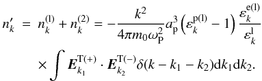 (33)The low-frequency longitudinal dielectric for electrons is
  when ωP ≫ ω ≫ kc (Mikhailovskii 1980). Therefore, Eq. (33) can be converted into
 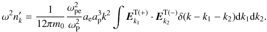 (34)In the case involving longitudinal fields, one needs to add the following term to the right-hand side of Eq. (15):
 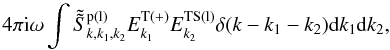 (35)in which
  is the same as
  , except that k2 is the four-dimensional wave vector for the low-frequency longitudinal field,
 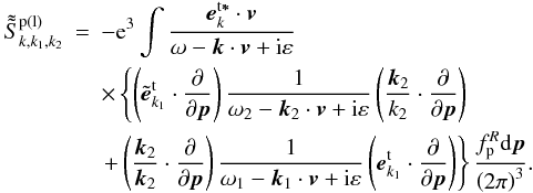 (36)Similarly as the derivation of interaction matrix
  , Eq. (36) can be simplified as
  (37)Considering Eqs. (29) and (37), Eq. (35) can be written as
  (38)Taking Eq. (38) into account, one obtains from Eq. (24)
  (39)For ω ≈ ωP ≫ kc, the transverse dielectric
  (Mikhailovskii 1980). Hence, Eq. ( 39) can be written as
  (40)
(40)
2.5. Nonlinear governing equation in coordinate space
For transverse plasmons near the frequency ωP, the high-frequency electric field  can be expressed as (Robinson 1997)
  (41)in which
  , and
, and  ,
,  varying very slowly compared with ωP is the complex envelope for the high-frequency fields. Using the following Fourier transformations
 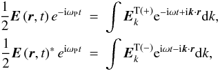 (42)Equations (34), (40) and (14) can be transformed into coordinate space
 ![Mathematical equation: \begin{eqnarray} \label{eq43} &&\frac{\partial ^2}{\partial t^2}\frac{n({{\vec r}},t)}{n_{\rm p0} } = c^2a_{\rm p}^2 \nabla ^2\frac{\left| {{{\vec E}}({{\vec r}},t)} \right|^2}{16\pi n_{\rm p0} T_{\rm e} }, \\ &&\frac{2\rm i}{\omega _{\rm P}}\frac{\partial }{\partial t}{{\vec E}}( {{\vec r}},t)-\frac{6}{5}\frac{c^{2}}{\omega _{\rm P}^{2}}\nabla \times \nabla \times {{\vec E}}({{\vec r}},t) \notag \\ &&-{\rm i}\frac{3}{a_{\rm p}}\frac{e}{m_{\rm p}\omega _{\rm P}c}\left\langle {\gamma _{\rm p}^{-4}} \right\rangle {{\vec E}}({{\vec r}},t)\times { {\vec B}}({{\vec r}},t)-3a_{\rm p}^{2}{{\vec E}}({ {\vec r}},t)\frac{{n}^{\prime }({{\vec r}},t)}{n_{\rm p0}} =0,~~~~~~~~~~~~ \label{eq44} \\ \label{eq45} &&\frac{\partial }{\partial t}{{\vec B}}({{\vec r}}{,}t) = {\rm i} \frac{3}{4}\frac{ec}{m_{\rm p} a_{\rm p} \omega _{\rm P}^2 } \Lambda \nabla \times \nabla \times [{{\vec E}}({{\vec r}},t)\times {{\vec E}} ^\ast ({{\vec r}},t)]. \end{eqnarray}](/articles/aa/full_html/2012/08/aa18921-12/aa18921-12-eq151.png) In deriving Eq. (44), we have neglected the term
In deriving Eq. (44), we have neglected the term  when the slow change envelope
  satisfies the condition ∂ln|E(r,t)|/∂t ≪ ωP. To obtain a real magnetic field with low-frequency, we have put ϕ = −π/2.
Introducing the following dimensionless parameters 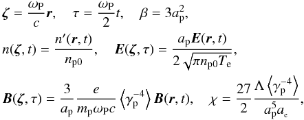 Equations (43), (44) and (45) can be transformed into
 ![Mathematical equation: \begin{eqnarray} \label{eq46} &&\frac{\partial ^2}{\partial \tau ^2}n({\rm {\bf \zeta }},\tau ) = \nabla ^2\left| {{{\vec E}}({\rm {\bf \zeta }},\tau )} \right|^2, \\ \label{eq47} &&{\rm i}\frac{\partial }{\partial \tau }{{\vec E}}({\rm {\bf \zeta }},\tau ) - \frac{6}{5} \nabla \times \nabla \times {\rm {\vec E}}({\rm {\bf \zeta }},\tau ) - \beta {{\vec E}}({\rm {\bf \zeta }},\tau )n({\rm {\bf \zeta }},\tau ) \nonumber\\ &&- {\rm i}{{\vec E}}({\rm {\bf \zeta }},\tau )\times {\vec B}({\rm {\bf \zeta }},\tau ) = 0, \\ \label{eq48} &&\frac{\partial }{\partial \tau }{\vec B}({\rm {\bf \zeta }},\tau ) = {\rm i}\chi \nabla \times \nabla \times [{\vec E}({\rm {\bf \zeta }},\tau )\times {{\vec E}}^\ast ({\rm {\bf \zeta }},\tau )]. \end{eqnarray}](/articles/aa/full_html/2012/08/aa18921-12/aa18921-12-eq157.png) Indeed, Eqs. (46)–(48) are a set of equations that can describe the magnetic field generated by the transverse plasmons in non-isothermal ultra-relativistic EP plasmas. Equation (46) characterizes the density variation caused by the divergence of ponderomotive force on the right side of Eq. (46). And Eq. (48) describes the evolution of the slowly varying magnetic field, which is set up by beats of the high-frequency transverse plasmons; as was discussed, the term E(ζ,τ) × E∗(ζ,τ) in (48) is the field “spin” (Thornhill & Haar 1978). The last term in the left-hand side of Eq. (47) describes the phase inhomogeneity via B(ζ,τ) and the third term represents the shift in plasma frequency caused by plasma density fluctuations.
Indeed, Eqs. (46)–(48) are a set of equations that can describe the magnetic field generated by the transverse plasmons in non-isothermal ultra-relativistic EP plasmas. Equation (46) characterizes the density variation caused by the divergence of ponderomotive force on the right side of Eq. (46). And Eq. (48) describes the evolution of the slowly varying magnetic field, which is set up by beats of the high-frequency transverse plasmons; as was discussed, the term E(ζ,τ) × E∗(ζ,τ) in (48) is the field “spin” (Thornhill & Haar 1978). The last term in the left-hand side of Eq. (47) describes the phase inhomogeneity via B(ζ,τ) and the third term represents the shift in plasma frequency caused by plasma density fluctuations.
We have followed the theory developed by Li & Ma (1993) in which the magnetic field is generated by transverse plasmons in non-relativistic regime. This theory had been generalized to the generation of magnetic field in plasmas containing ultra-relativistic electrons and non-relativistic ions (Li et al. 2008), and used to investigate the nonlinear behavior of transverse plasmons in isothermal ultra-relativistic EP plasmas (Liu & Liu 2011). If similar physical processes are taken into account, there are some similarities between the paper and those mentioned above. However, our work is different from the previous works in the following aspects:
-
1)
the special relativistic theory limits the particle speed to lessthan the speed of light, which allows us to calculate the integrals inthe interaction matrix for a fully relativistic regime by focusingour analysis on the large-scale superluminal waves; i.e.,kc ≪ ω, which is different from the papers mentioned above;
-
2)
the net nonlinear magnetization currents in the paper are determined by ultra-relativistic positrons, whereas in the works of Li & Ma (1993) and Li et al. (2008), it is dominantly produced by non-relativistic electrons and by non-relativistic ions, respectively. In the case of isothermal EP plasmas, there are no net nonlinear magnetization currents (Liu & Liu 2011).
3. Linear analysis for transverse perturbations
Now we examine the problem of the stability of monochromatic waves in the Liapunov sense in the framework of Eqs. (46)–(48). It is easily examined that the following form of plane wave, ![Mathematical equation: \begin{equation} \label{eq49} {{\vec E}}_0 = {{\vec E}}_{00} \exp \left[ {{\rm i}\left( {{{\vec k}}_0 \cdot {\rm {\bf \xi }} - \omega _0 \tau } \right)} \right], \quad {\vec B}_0 = 0, \quad n_0 = 0, \end{equation}](/articles/aa/full_html/2012/08/aa18921-12/aa18921-12-eq161.png) (49)is a solution of Eqs. (46)–(48), provided that
(49)is a solution of Eqs. (46)–(48), provided that 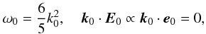 (50)e0 is a unit vector:
  .
.
To investigate the stability of the solution, we assume the presence of small perturbations (δE, δB, δn) to the solution, if the disturbance is amplified, then the solution is unstable in the Liapunov sense. Linearizing Eqs. (46)–(48) with respect to the perturbations yields ![Mathematical equation: \begin{eqnarray} \label{eq51} &&(\delta n )_{\tau \tau } = \nabla ^2[{{\vec E}}_{0} \cdot \delta {{\vec E}}^\ast + {{\vec E}}_{0}^\ast \cdot \delta {{\vec E}} ], \\ \label{eq52} &&{\rm i}(\delta {{\vec E}} )_\tau - \nabla \times \nabla \times \delta {{\vec E}} = \beta \delta n {{\vec E}}_{0} + {\rm i}{{\vec E}}_{0} \times \delta {\vec B}, \\ \label{eq53} &&(\delta {\vec B} )_\tau = {\rm i}\chi \nabla \times \nabla \times [{{\vec E}}_{0} \times \delta {{\vec E}}^\ast + \delta {{\vec E}} \times {{\vec E}}_{0}^\ast ]. \end{eqnarray}](/articles/aa/full_html/2012/08/aa18921-12/aa18921-12-eq168.png) We study the following forms of the transverse perturbations:
We study the following forms of the transverse perturbations: ![Mathematical equation: \begin{eqnarray} \label{eq54} \delta n &=& \frac{1}{2}n\left\{ {\exp [{\rm i}({{\vec k}} \cdot {\rm {\bf \xi }} - \omega \tau )] + \exp [ - {\rm i}({{\vec k}} \cdot {\rm {\bf \xi }} - \omega \tau )]} \right\}, \\ \label{eq55} \delta {\vec B} &=& \frac{1}{2}{\vec B}\left\{ {\exp [{\rm i}({{\vec k}} \cdot {\rm {\bf \xi }} - \omega \tau )] + \exp [ - {\rm i}({{\vec k}} \cdot {\rm {\bf \xi }} - \omega \tau )]} \right\}, \\ \delta {{\vec E}} &=&\left\{ {{{\vec E}}\exp [{\rm i}({ {\vec k}}\cdot {{\vec \xi }}-\omega \tau )]+{{\vec E}} ^{+}\exp [-{\rm i}({{\vec k}}\cdot {{\vec \xi }}-\omega \tau )]} \right\} \notag \\ &&\quad\times \exp [{\rm i}({{\vec k}}_{0}\cdot {{\vec \xi }}-\omega _{0}\tau )], \label{eq56} \end{eqnarray}](/articles/aa/full_html/2012/08/aa18921-12/aa18921-12-eq169.png) where E, E + are transverse perturbations:
where E, E + are transverse perturbations:  (57)where e1,
  are real unit vectors.
Substituting Eqs. (49), (50), (54) and (56) into Eq. (51) yields ![Mathematical equation: \begin{equation} \label{eq58} \frac{n}{2}\omega ^2 = k^2[E({{\vec e}}_2^ + \cdot {{\vec E}}_{00} ) + E({{\vec e}}_1 \cdot {\vec E}_{00}^\ast )]. \end{equation}](/articles/aa/full_html/2012/08/aa18921-12/aa18921-12-eq175.png) (58)Similarly, we obtain from Eq. (52),
(58)Similarly, we obtain from Eq. (52), 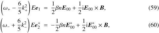 where
where  (61)Combining Eqs. (58)–(61), one can obtain
 ![Mathematical equation: \begin{equation} \label{eq63} n\left[ {\omega ^2 - \frac{\frac{12}{5}\beta k^4\left| {{{\vec E}}_{00} } \right|^2}{(\omega - \frac{12}{5}{{\vec k}} \cdot {{\vec k}}_0 )^2 -\frac{36}{25} k^4}} \right] = - {\rm i}\frac{\frac{12}{5}k^4{\vec B} \cdot ({{\vec E}}_{00} \times {{\vec E}}_{00}^\ast )}{(\omega - \frac{12}{5}{{\vec k}} \cdot {{\vec k}}_0 )^2 -\frac{36}{25} k^4}\cdot \end{equation}](/articles/aa/full_html/2012/08/aa18921-12/aa18921-12-eq178.png) (62)From Eq. (53), we easily arrive at
(62)From Eq. (53), we easily arrive at ![Mathematical equation: \begin{eqnarray} \omega {{\vec B}} &=&2\chi k^{2}EE_{00}\left[ {({{\vec e}} _{2}^{+}\times {{\vec e}}_{0})-\frac{E_{00}^{\ast }}{E_{00}}({ {\vec e}}_{1}\times {{\vec e}}_{0}^{\ast })}\right. \notag \\ &&\left. {+\frac{E_{00}^{\ast }}{E_{00}}{{\vec e}}_{{{k} }}{{\vec e}}_{{k}}\cdot ({{\vec e}} _{1}\times {{\vec e}}_{0}^{\ast })-{{\vec e}}_{{ {k}}}{{\vec e}}_{{k}}\cdot ({{\vec e }}_{2}^{+}\times {{\vec e}}_{0})}\right]. \label{eq64} \end{eqnarray}](/articles/aa/full_html/2012/08/aa18921-12/aa18921-12-eq179.png) (63)Doting the both sides of Eq. (63) with
(63)Doting the both sides of Eq. (63) with  yields
  (64)where
 ![Mathematical equation: \begin{eqnarray} G &=&[({{\vec e}}_{2}^{+}\cdot {{\vec e}}_{0})-({ {\vec e}}_{2}^{+}\cdot {{\vec e}}_{0}^{\ast })({{\vec e}} _{0}\cdot {{\vec e}}_{0})] \notag \\ &&-\frac{E_{00}^{\ast }}{E_{00}}[({{\vec e}}_{1}\cdot {{\vec e}}_{0})({{\vec e}}_{0}^{\ast }\cdot {{\vec e}}_{0}^{\ast })-({{\vec e}}_{1}\cdot {{\vec e}}_{0}^{\ast })] \notag \\ &&+\frac{E_{00}^{\ast }}{E_{00}}[{{\vec e}}_{{k} }\cdot ({{\vec e}}_{0}\times {{\vec e}}_{0}^{\ast })][ {{\vec e}}_{{k}}\cdot ({{\vec e}} _{1}\times {{\vec e}}_{0}^{\ast })] \notag \\ &&-[{{\vec e}}_{{k}}\cdot ({{\vec e}} _{0}\times {{\vec e}}_{0}^{\ast })][{{\vec e}}_{{ {\vec k}}}\cdot ({{\vec e}}_{2}^{+}\times {{\vec e}} _{0})]. \label{eq67} \end{eqnarray}](/articles/aa/full_html/2012/08/aa18921-12/aa18921-12-eq182.png) (65)Equations (60) and (64) yield
(65)Equations (60) and (64) yield  (66)Therefore, the following dispersion relation
 ![Mathematical equation: \begin{eqnarray} &&\left[ {\left(\omega +k^{2}-\frac{12}{5}{{\vec k}}\cdot {{\vec k}}_{0}\right) {{\vec e}}_{2}^{+}\cdot {{\vec e}}_{0}-{\rm i}\chi \left\vert { {{\vec E}}_{00}}\right\vert ^{2}G\frac{k^{2}}{\omega }}\right] \nonumber \\ &&\times\left[ {\omega ^{2}-\frac{\frac{12}{5}\beta k^{4}\left\vert {{{\vec E}}_{00}} \right\vert ^{2}}{(\omega -\frac{12}{5}{{\vec k}}\cdot {{\vec k}} _{0})^{2}-\frac{36}{25}k^{4}}}\right] =\nonumber\\ &&\hspace*{3mm}{\rm i}\frac{\frac{12}{5}\chi \beta \left\vert {{{\vec E }}_{00}}\right\vert ^{4}G}{(\omega -\frac{12}{5}{{\vec k}}\cdot {{\vec k}}_{0})^{2}-\frac{36}{25}k^{4}}\frac{k^{6}}{\omega } \label{eq69} \end{eqnarray}](/articles/aa/full_html/2012/08/aa18921-12/aa18921-12-eq184.png) (67)can be obtained from Eqs. (62), (64) and (66). The dispersion Eq. (67) is quite complicated in general. For the purpose of obtaining a simple analytical result, we assume e0 is a real vector. Now, the dispersion Eq. (67) is reduced to
(67)can be obtained from Eqs. (62), (64) and (66). The dispersion Eq. (67) is quite complicated in general. For the purpose of obtaining a simple analytical result, we assume e0 is a real vector. Now, the dispersion Eq. (67) is reduced to  (68)where θ is the angle between k and k0. If one takes θ = π/2, the above equation can be written as
  (69)The roots of Eq. (69) are
 ![Mathematical equation: \begin{equation} \label{eq72} \omega ^2 =\frac{18}{25}k^4\left[ {1\pm \sqrt {1 + \frac{250}{54}\beta \left| {{{\vec E}}_{00} } \right|^2 / k^4} } \right]. \end{equation}](/articles/aa/full_html/2012/08/aa18921-12/aa18921-12-eq191.png) (70)Obviously, Eq. (70) has imaginary roots, i.e., there will be instability. From Eq. (70) we obtain the instability growth rate, Γ = Im(ω),
(70)Obviously, Eq. (70) has imaginary roots, i.e., there will be instability. From Eq. (70) we obtain the instability growth rate, Γ = Im(ω), ![Mathematical equation: \begin{equation} \label{eq73} \Gamma ^2 = \frac{18}{25}k^4\left[ {\sqrt {1 + \frac{250}{54}\beta \left| {{{\vec E}}_{00} } \right|^2 / k^4}-1 } \right]. \end{equation}](/articles/aa/full_html/2012/08/aa18921-12/aa18921-12-eq193.png) (71)From above analysis, one can conclude that the spontaneous magnetic field is modulationally unstable. Naturally, the mode with the highest growth rate, Γmax, dominates and sets the characteristic length scale of the magnetic field fluctuations, xc ~ 1/kmax, kmax is the wave number at which the maximum growth rate occurs. The ultrarelativistic expressions for Γmax and kmax are given by Eq. (67). The dispersion Eq. (67) is so complicated that numerical calculation is the only way to obtain a general knowledge of the growth rate and characteristic scale of self-generated magnetic field.
(71)From above analysis, one can conclude that the spontaneous magnetic field is modulationally unstable. Naturally, the mode with the highest growth rate, Γmax, dominates and sets the characteristic length scale of the magnetic field fluctuations, xc ~ 1/kmax, kmax is the wave number at which the maximum growth rate occurs. The ultrarelativistic expressions for Γmax and kmax are given by Eq. (67). The dispersion Eq. (67) is so complicated that numerical calculation is the only way to obtain a general knowledge of the growth rate and characteristic scale of self-generated magnetic field.
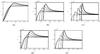 |
Fig. 1 Growth rate with respect to the wave number calculated from Eq. (68). The different lines in each figure correspond to different θ. a) W0 = 0.1,ap = 0.05, b) W0 = 0.1,ap = 0.02, c) W0 = 0.1,ap = 0.01, d) W0 = 0.01,ap = 0.05, e) W0 = 0.001,ap = 0.05. |
During numerical calculation we find that the maximum growth rate and the corresponding kmax obtained from Eq. (67) are weakly depended on ae, and the results are similar to that calculated from Eq. (68). It means the terms containing χ in Eq. (67) are negligible. In the following, the dispersion curves for different values of ap and  are presented in accordance with Eq. (68). Figure 1 shows the growth rate of modulation instability with respect to k for k0 = 0.05 and θ varies from 0 to π. Figures 1a–c are calculated at ap = 0.05, 0.02 and 0.01, respectively, in which
  . Figures 1d, and e are calculated at
  and 0.001, respectively, in which ap = 0.05. The maximum growth rate and corresponding characteristic scale in units of ωP/2 and c/ωP are 4.4 × 10⁻³ and 7.2 for Fig. 1a, 1.1 × 10⁻³ and 9.5 for Fig. 1b, 4.3 × 10⁻⁴ and 9.8 for Fig. 1c, 1.8 × 10⁻³ and 9.0 for Fig. 1d, and 8.0 × 10⁻⁴ and 9.7 for Fig. 1e.
With increasing positrons temperature, the scale of the magnetic field will increase, and the growth rate will decrease, as can be seen from Figs. 1a–c. In contrast, increasing the amplitude of the wave field results in the decrease of the magnetic field scale and an increase of the growth rate. Therefore, one can conclude that strong turbulence fields favor of the generation of strong localized magnetic field. The modulation instability and the growth rate should be determined by the temperature difference of electrons and positrons, whereas the assumption of Te ≫ Tp leads them to weakly depend on the electron temperature. If the difference of temperature is finite, the effects of electrons on the nonlinear currents should be taken into consideration.
4. Discussions and conclusions
The modulation interaction between the transverse plasmons and the low-frequency density fluctuation will lead the wave field collapse into a localized rarified region where the strong wave field is trapped. In the density caviton there will be a strong highly intermittent magnetic field, which can be inferred from Eq. (48). Regarding this, we seek a self-similar collapse solution for the nonlinear self-generated magnetic field within the framework of Eqs. (46)–(48). Assuming the characteristic time-space scales of n, E and B to be τ and ζ, then from Eqs. (46) and (48) one has 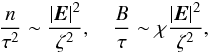 (72)where τ′ = τ0 − τ, τ0 corresponds to the final state of collapse, as mentioned above, the perturbed fields become too strong for the condition of Eq. (2) to be valid.
Using Eq. (72), the order of magnitudes of the terms in Eq. (47) can be read as 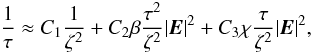 (73)where C1, C2 and C3 are constants on the order of unity. One can readily derive
  , provided that the first term and the last term in the right-hand side of Eq. (73) are balanced, which implies
  (74)Therefore, there is
  (75)From the Eq. (47), one can obtain
 ![Mathematical equation: \begin{eqnarray} &{\rm i}\frac{\partial }{\partial \tau }\left\vert {{{\vec E}}({ {\vec \zeta }},\tau )}\right\vert ^{2}+\frac{6 }{5 }\nabla \cdot \left[ {\left( {\nabla \times {{\vec E}}^{\ast }({{\vec \zeta }},\tau )}\right) \times {{\vec E}}({{\vec \zeta }},\tau )}\right. \notag \\ &\left. {-\left( {\nabla \times {{\vec E}}({{\vec \zeta }} ,\tau )}\right) \times {{\vec E}}^{\ast }({{\vec \zeta }} ,\tau )}\right] =0. \label{eq78} \end{eqnarray}](/articles/aa/full_html/2012/08/aa18921-12/aa18921-12-eq241.png) (76)Integrating the above equation over all space yields the conservation of the plasmon number
(76)Integrating the above equation over all space yields the conservation of the plasmon number  Generally, the modulational instability will lead to an anisotropic collapse of the magnetic field, resulting in an pancake-like structure with a scale ζ and radius R (R ≫ ζ). This leads to
  (77)We try to find a solution in the form
 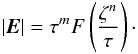 (78)Then, Eqs. (74) and (77) become
  (79)Taking account of the Eq. (74), one derives
  and n = 1. Thus, a self-similar collapse solution can be asymptotically shown as
  (80)with R ~ const. Here, F is a function determined by the initial conditions. Assuming ζf is the scale to stop the collapse, the maximum growth rate
  by the nonlinear collapse motion could be obtained from the self-similar Eq. (80) as
  (81)There is evidence that the nonlinear collapse growth rate is always higher than that of the linear instability (Li & Ma 1993; Li et al. 2008), which results in ζf < xc.
The magnitude of the magnetic field in dimensionless form can be estimated from Eq. (48) as  (82)where
  is the wave density in the final state. In dimensional units,
 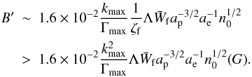 (83)For the magnetic field in the internal shock region of GRB, one may take the characteristic Lorentz factor for electrons to be
  , and the particle density for electrons and positrons n0 ~ 3 × 1010 cm-3 (Medvedev & Loeb 1999). Assuming
  and the initial wave density , the dimensionless maximum growth rate and the corresponding wave number from Fig. 1b are Γmax = 1.1 × 10⁻³ and kmax = 0.105, respectively. The dimensional growth rate of the spontaneous magnetic field is
  . The characteristic e-folding time for the field (~10-6 s) is much shorter than the duration parameter T90, which is the time over which a burst emits from 5% of its total measured counts to 95%. This means that the self-generated magnetic field can be assumed to be invariant with time during T90. In addition, the characteristic scale of the magnetic field is xc ~ 3.6 × 102 cm. Taking the final wave density in a localized region to be
  , the magnitude of this magnetic field is probably higher than 104 G. Our results are consistent with the prediction made by Deng et al. (2005). In their model, gamma-ray burst spectra can be explained by the synchro-curvature mechanism with the curvature and the strength of magnetic field to be ~100 cm and 104 G respectively. In conclusion, we have investigated the nonlinear evolution of EM turbulence with frequency ω ≈ ωP in the non-isothermal ultra-relativistic EP plasma from a kinetic way. We revealed that the coupling of transverse plasmons, low-frequency density perturbation, and spontaneous magnetic field that arise from the nonlinear wave-wave and wave-particle interactions can be self-consistently described by Eqs. (46)–(48). The linear stability analysis showed that the transverse perturbation is modulation-unstable, which will lead the magnetic field to grow and form spatially highly intermittent magnetic fluxes. The instability, weakly depending on the spontaneous magnetic field, is dominantly caused by the modulation interaction between the transverse plasmons and the low-frequency density perturbation. Our numerical results imply that the growth rate of the instability and the characteristic scale of the magnetic field are determined by the field intensity and the effective temperature of the positrons. The characteristic scale is much larger than that of the Weibel instability, which is on the order of the collisionless skin depth. The Landau damping of the field will be much weaker than that of the field generated by Weibel instability, which is conducive to the generation of the long-life small-scale magnetic fields in the internal shock region of GRBs. The results we obtained can give a plausible explanation for the origin of the long-term small-scale magnetic field needed to explain the prompt GMBs spectrum. We focused on the generation of the small-scale magnetic field in the region of the internal shock of GRBs by transverse plasmons. The macro-equipartition parameters and the macro-energy transfer, including energy dissipation along the GRB jet and the temporal variability observed in GRBs, are beyond the main purpose of our manuscript, and we will investigate these significant problems in future. It is worth noting that our model is based on the different temperature of electrons and the positrons; this point needs an additional confirmation from observations.
Acknowledgments
The project was supported by the International S&T Cooperation Program of China (2009DFA02320), Program for Innovative Research Team in Jiangxi Province (2010DQB00900), the National Basic Research Program of China (973 Program) (No. 2010CB635112) and National Natural Science Foundation of China under grant No. 11178002.
References
- Chang, P., Spitkovsky, A., & Arons, J. 2008, ApJ, 674, 378 [Google Scholar]
- Cohen, E. J., Katz, I., Piran, T., et al. 1997, ApJ, 488, 330 [NASA ADS] [CrossRef] [Google Scholar]
- Deng, X. L., Xia, T. S., & Liu, J. 2005, A&A, 443, 747 [NASA ADS] [CrossRef] [EDP Sciences] [Google Scholar]
- Ghisellini, G., Celotti, A., & Lazzati, D. 2000, MNRAS, 313, L1 [NASA ADS] [CrossRef] [Google Scholar]
- Gruzinov, A. 2001, ApJ, 563, L15 [NASA ADS] [CrossRef] [Google Scholar]
- Jüttner, F. 1911, Ann. der Phys., 34, 856 [Google Scholar]
- Kaplan, S. A., & Tsytovich, V. N. 1973, Plasma Astrophysics (London: Pergamon Press) [Google Scholar]
- Karpman, V. I., Norman, C. A., ter Haar, D., & Tsytovich, V. N. 1975, Phys. Scripta, 11, 271 [Google Scholar]
- Katz, B., Keshet, U., & Waxman, E. 2007, ApJ, 655, 375 [NASA ADS] [CrossRef] [Google Scholar]
- Li, X. Q., & Ma, Y. H. 1993, A&A, 270, 534 [NASA ADS] [Google Scholar]
- Li, X. Q., Liu, S. Q., & Tao, X. Y. 2008, Contrib. Plasma Phys., 48, 361 [NASA ADS] [CrossRef] [Google Scholar]
- Liang, E. P. 1982, Nature, 299, 321 [NASA ADS] [CrossRef] [Google Scholar]
- Lifshitz, E. N., & Pitaevskii, L. P. 1981, Physical Kinetics (Oxford: Pergamon Press) [Google Scholar]
- Liu, Y., & Liu, S. Q. 2011, Contrib. Plasma Phys., 51, 698 [NASA ADS] [CrossRef] [Google Scholar]
- Liu, X. L., Liu, S. Q., & Yang, X. S. 2008, Phys. Plasmas, 15, 032302 [NASA ADS] [CrossRef] [Google Scholar]
- Mao, J., & Wang, J. 2011, ApJ, 731, 26 [NASA ADS] [CrossRef] [Google Scholar]
- Medvedev, M. V. 2000, ApJ, 540, 704 [NASA ADS] [CrossRef] [Google Scholar]
- Medvedev, M. V. 2006, ApJ, 637, 869 [NASA ADS] [CrossRef] [Google Scholar]
- Medvedev, M. V., & Loeb, A. 1999, ApJ, 526, 697 [NASA ADS] [CrossRef] [Google Scholar]
- Medvedev, M. V., Fiore, M., Fonseca, R. A., Silva, L. O., & Mori, W. B. 2005, ApJ, 618, L75 [NASA ADS] [CrossRef] [Google Scholar]
- Mikhailovskii, A. B. 1980, Plasma Phys., 22, 133 [NASA ADS] [CrossRef] [Google Scholar]
- Morsony, B. J., Workman, J. C., Lazzati, D., & Medvedev, M. V. 2009, MNRAS, 392, 1397 [NASA ADS] [CrossRef] [Google Scholar]
- O’Neil, T. M., & Coroniti, F. V. 1999, Rev. Mod. Phys., 71, S404 [CrossRef] [Google Scholar]
- Pe’er, A., & Zhang, B. 2006, ApJ, 653, 454 [NASA ADS] [CrossRef] [Google Scholar]
- Pulupa, M. P., Bale, S. D., & Kasper, J. C. 2010, J. Geophys. Res., 115, A04106 [NASA ADS] [Google Scholar]
- Robinson, P. A. 1997, Rev. Mod. Phys., 69, 507 [NASA ADS] [CrossRef] [Google Scholar]
- Silva, L. O., Fonseca, R. A., Tonge, J. W., et al. 2003, ApJ, 596, L121 [Google Scholar]
- Thornhill, S. G., & Ter Haar, D. 1978, Phys. Rep., 43, 43 [NASA ADS] [CrossRef] [Google Scholar]
- Tkaczyk, W. 1993 Unthermalized Plasma in Phebus and BATSE Gamma Ray Bursts Sources. 23rd International Cosmic Ray Conference, 1, eds. D. A. Leahy, R. B. Hickws, & D. Venkatesan (Singapore: World Scientific), 124 [Google Scholar]
- Tsytovich, V. N. 1977, Theory of turbulent plasma (New York: Consultants Bureau) [Google Scholar]
- Workman, J. C., Morsony, B. J., Lazzati, D., & Medvedev, M. V. 2008, MNRAS, 386, 199 [NASA ADS] [CrossRef] [Google Scholar]
Appendix A: Calculation of the matrix 
Expanding the differentiation in close brackets of Eq. (11), one can obtain 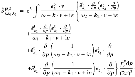 (A.1)We define
 ![Mathematical equation: \appendix \setcounter{section}{1} \begin{eqnarray} H &=&\left[ \frac{1}{\omega _{2}-{{\vec k}}_{2}\cdot { {\vec v}}}{\left( {{\tilde{{\vec e}}}_{{k} _{2}}^{\rm t}\cdot \frac{\partial }{\partial {{\vec p}}}}\right) \left( {{{\vec e}}_{{k}_{1}}^{\rm t}\cdot \frac{\partial }{ \partial {{\vec p}}}}\right) }\right. \notag \\ &&\left. {+\frac{1}{\omega _{1}-{{\vec k}}_{1}\cdot {{\vec v}}}\left( {{\tilde{{\vec e}}}_{{k}_{1}}^{\rm t}\cdot \frac{\partial }{\partial {{\vec p}}}}\right) \left( {{ {\vec e}}_{{k}_{2}}^{\rm t}\cdot \frac{\partial }{\partial {{\vec p}}}}\right) }\right] f_{\rm p}^{R}. \label{eqa2} \end{eqnarray}](/articles/aa/full_html/2012/08/aa18921-12/aa18921-12-eq276.png) (A.2)For positive high-frequency and negative high-frequency transverse fields with ω1 ≈ − ω2 ≈ ωP ≫ kc, Eq. ( A.2) can be written as
(A.2)For positive high-frequency and negative high-frequency transverse fields with ω1 ≈ − ω2 ≈ ωP ≫ kc, Eq. ( A.2) can be written as ![Mathematical equation: \begin{equation*} H \approx \frac{1}{\omega _{\rm P} }\left[ {\left( {{\tilde {{\vec e}}}_{ {k}_2 }^{\rm t} \cdot \frac{\partial }{\partial {{\vec p}} }} \right)\left( {{{\vec e}}_{{k}_1 }^{\rm t} \cdot \frac{ \partial }{\partial {{\vec p}}}} \right) - \left( {{\tilde { {\vec e}}}_{{k}_1 }^{\rm t} \cdot \frac{\partial }{\partial {{\vec p}}}} \right)\left( {{{\vec e}}_{{k} _2 }^{\rm t} \cdot \frac{\partial }{\partial {{\vec p}}}} \right)} \right] f_{\rm p} ^R. \end{equation*}](/articles/aa/full_html/2012/08/aa18921-12/aa18921-12-eq278.png) Under the high-frequency approximation, there are
Under the high-frequency approximation, there are  and
and  . Now, it is easy to obtain H ≈ 0. Therefore, Eq. (A.1) can be reduced to
 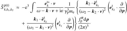 (A.3)When the equilibrium distribution of positrons (
 ) is isotropic, one has
  . Under the high-frequency approximation, Eq. (A.3) can be written as
 ![Mathematical equation: \appendix \setcounter{section}{1} \begin{eqnarray} \tilde{S}_{k,k_{1},k_{2}}^{\rm p\left( {t}\right) } &\approx &-{\rm e}^{3}\int {\frac{1 }{\gamma _{\rm p}^{3}m_{\rm e}}\frac{1}{\omega -{{\vec k}}\cdot { {\vec v}}+{\rm i}\varepsilon }\left[ {\frac{\left( {{{\vec k}}_{{ 2}}\cdot {{\vec e}}_{{k}_{1}}^{\rm t}}\right) \left( { {{\vec e}}_{{k}_{2}}^{\rm t}\cdot {{\vec v}}} \right) }{\left( {\omega _{2}-{{\vec k}}_{2}\cdot {{\vec v} }}\right) ^{2}}}\right. } \notag \\ &&+\left. \frac{\left( {{{\vec k}}_{1}\cdot {{\vec e}}_{ {k}_{2}}^{\rm t}}\right) \left( {{{\vec e}}_{{ {\vec k}}_{1}}^{\rm t}\cdot {{\vec v}}}\right) }{\left( {\omega _{1}- {{\vec k}}_{1}\cdot {{\vec v}}}\right) ^{2}}\right] \left( {{{\vec e}}_{k}^{\rm t\ast }\cdot \frac{\partial }{\partial { {\vec p}}}}\right) f_{\rm p}^{R}\frac{{\rm d}{{\vec p}}}{\left( {2\pi } \right) ^{3}}\cdot \label{eqa4} \end{eqnarray}](/articles/aa/full_html/2012/08/aa18921-12/aa18921-12-eq285.png) (A.4)Taking account of |ω1| ≈ |ω2| ≈ ωP ≫ kc, the above equation can be approximated to be
(A.4)Taking account of |ω1| ≈ |ω2| ≈ ωP ≫ kc, the above equation can be approximated to be ![Mathematical equation: \appendix \setcounter{section}{1} \begin{eqnarray} \tilde{S}_{k,k_{1},k_{2}}^{\rm p\left( {t}\right) } &\approx &-\frac{{\rm e}^{3}}{ m_{\rm e}\omega _{{P}}^{{2}}}\int {\frac{\left[ {\left( {{{\vec k}} _{2}\cdot {{\vec e}}_{{k}_{1}}^{\rm t}}\right) \left( { {{\vec e}}_{{k}_{2}}^{\rm t}\cdot {{\vec v}}} \right) +\left( {{{\vec k}}_{1}\cdot {{\vec e}}_{{ {k}}_{2}}^{\rm t}}\right) \left( {{{\vec e}}_{{k} _{1}}^{\rm t}\cdot {{\vec v}}}\right) }\right] }{\gamma _{\rm p}^{3}{\left( \omega -{{\vec k}}\cdot {{\vec v}}+{\rm i}\varepsilon \right) }}} \notag \\ &&\left( {{{\vec e}}_{k}^{\rm t\ast }\cdot \frac{\partial }{\partial {{\vec p}}}}\right) f_{\rm p}^{R}\frac{{\rm d}{{\vec p}}}{\left( { 2\pi }\right) ^{3}}\cdot \label{eqa5} \end{eqnarray}](/articles/aa/full_html/2012/08/aa18921-12/aa18921-12-eq287.png) (A.5)After integration by parts, there is
(A.5)After integration by parts, there is ![Mathematical equation: \appendix \setcounter{section}{1} \begin{eqnarray} &&\tilde{S}_{k,k_{1},k_{2}}^{\rm p\left( {t}\right) } =\frac{{\rm e}^{3}}{ m_{\rm e}^{2}\omega _{\rm P}^{2}}\int {\frac{{1}}{\gamma _{\rm p}^{3}}\left( {{ {\vec e}}_{k}^{\rm t\ast }\cdot \frac{\partial }{\partial {{\vec v}}}} \right) } \notag \\ &&\times{\left\{ {\frac{{\left[ {\left( {{{\vec k}}_{2}\cdot { {\vec e}}_{{k}_{1}}^{\rm t}}\right) \left( {{{\vec e}} _{{k}_{2}}^{\rm t}\cdot {{\vec v}}}\right) +\left( { {{\vec k}}_{1}\cdot {{\vec e}}_{{k} _{2}}^{\rm t}}\right) \left( {{{\vec e}}_{{k} _{1}}^{\rm t}\cdot {{\vec v}}}\right) }\right] }}{\gamma _{\rm p}^{3}{ \left( \omega -{{\vec k}}\cdot {{\vec v}}+{\rm i}\varepsilon \right) }}}\right\} }\frac{f_{\rm p}^{R}{\rm d}{{\vec p}}}{\left( {2\pi } \right) ^{3}}\cdot \label{eqa6} \end{eqnarray}](/articles/aa/full_html/2012/08/aa18921-12/aa18921-12-eq288.png) (A.6)After a series of algebraic calculations, and considering ω ≫ kc, Eq. (A.6) can be written as
(A.6)After a series of algebraic calculations, and considering ω ≫ kc, Eq. (A.6) can be written as ![Mathematical equation: \appendix \setcounter{section}{1} \begin{eqnarray} \tilde{S}_{k,k_{1},k_{2}}^{\rm p\left( {t}\right) } &\approx &\frac{{\rm e}^{3}}{ m_{\rm e}^{{2}}\omega _{{\rm P}}^{{2}}\omega }\Biggl\{ {{\int {\frac{3}{\gamma _{\rm p }^{4}}\left[ {\left( {{{\vec e}}_{{k} _{1}}^{\rm t}\times {{\vec e}}_{{k}_{2}}^{\rm t}}\right) \cdot \left( {{\vec {k}}\times {{\vec v}}}\right) \left( { {\vec {e}}_{k}^{\rm t\ast }\cdot {{\vec v}}}\right) }\right] } \frac{f_{\rm p}^{R}}{c^{2}}\frac{{\rm d}{\vec {p}}}{\left( {2\pi }\right) ^{3} }}} \nonumber \\ &&{+} {{n_{0}{\vec {e}}_{k}^{\rm t\ast }\cdot \left[ {{ \vec {e}}_{{{k}}_{2}}^{\rm t}\left( {{\vec {k}}_{ 2}\cdot {\vec {e}}_{{{k}}_{1}}^{\rm t}} \right) +{\vec {e}}_{{{k}}_{1 }}^{\rm t}\left( {{\vec {k}}_{1}\cdot {\vec {e}}_{{ {k}}_{2}}^{\rm t}}\right) }\right] \left\langle {\gamma _{\rm p}^{-6}} \right\rangle }}\Biggl\} \label{eqa7}. \end{eqnarray}](/articles/aa/full_html/2012/08/aa18921-12/aa18921-12-eq290.png) (A.7)The first term on the right-hand side of Eq. (A.7) can be read as
(A.7)The first term on the right-hand side of Eq. (A.7) can be read as  (A.8)where the following expression has been used
  (A.9)Taking the δ-function in Eq. (11) into account, one can arrive at k2 = k1 − k, in which k1 and k2 are positive and negative wave vectors, respectively. Thus, the second term on the right-hand side of (A.7) can be reduced to
 ![Mathematical equation: \appendix \setcounter{section}{1} \begin{equation} \label{eqa10} \frac{{\rm e}^3n_0 }{m_{\rm e}^{2} \omega \omega _{\rm P}^{2} }{\vec {e}}_{k}^{\rm t\ast } \cdot \left[ {{\vec {e}}_{{{k}}_2 }^{\rm t} \left( { {\vec {k}}_{2} \cdot {\vec {e}}_{{ {k}}_1 }^{\rm t} } \right) + {\vec {e}}_{{{k}}_{ 1} }^{\rm t} \left( {{{\vec k}}_1 \cdot {\vec { e}}_{{{k}}_2 }^{\rm t} } \right)} \right]\left\langle {\gamma _{\rm p}^{{\ - 6}} } \right\rangle. \end{equation}](/articles/aa/full_html/2012/08/aa18921-12/aa18921-12-eq296.png) (A.10)Combining (A.8) and (A.10) yields
(A.10)Combining (A.8) and (A.10) yields ![Mathematical equation: \appendix \setcounter{section}{1} \begin{equation} \label{eqa11} \tilde {S}_{k,k_1 ,k_2 }^{\rm p \left( {t} \right)} = - \frac{{\rm e}^3n_0 }{ m_{\rm e}^{2} \omega \omega _{\rm P}^{2} }{\vec {e}}_{k}^{\rm t\ast } \cdot \left[ { {\vec {k}}\times \left( {{\vec {e}}_{{{k}}_1 }^{\rm t} \times {\vec {e}}_{{{k}}_2 }^{\rm t} } \right)} \right] \left( {\left\langle {\gamma _{\rm p}^{{\ - 4}} } \right\rangle - 2\left\langle { \gamma _{\rm p}^{{\ - 6}} } \right\rangle } \right). \end{equation}](/articles/aa/full_html/2012/08/aa18921-12/aa18921-12-eq297.png) (A.11)
(A.11)
Appendix B: Calculation of the matrix 
The matrix  can be written as
  (B.1)in which
  (B.2)
(B.2) (B.3)where k1 = (k1,ω1) and k = (k,ω) are four-dimensional wave vectors for the high-frequency transverse field, k2 = (k2,ω2) is the four-dimensional wave vector for the low-frequency transverse field.
Integrating Eq. (B.2) by parts, and considering ω ≫ kc, one derives  (B.4)Integrating Eq. (B.4) by parts, and considering
  if kc ≪ ω1 ≈ ωP, Eq. (B.4) can be read as
  (B.5)For the transverse field, i.e.
  , and considering the facts ω2 ≫ k2c, there is
  (B.6)In view of the isotropic distribution of the positrons in equilibrium state, it is easy to obtain S1 = 0.
Integrating Eq. (B.3) by parts, if k1c ≪ ω1 ≈ ωP, similarly as the calculation of Eq. (B.4), one can obtain  (B.7)Integrating the above equation by parts, one derives
 ![Mathematical equation: \appendix \setcounter{section}{2} \begin{eqnarray} &&S_{2}=-\frac{{\rm e}^{3}}{\omega m_{\rm p}^{2}\omega _{1}}\int {\frac{1}{\gamma _{\rm p}^{6}}\left( {{{\vec e}}_{k_{1}}^{\rm t}\cdot \frac{\partial }{\partial {{\vec v}}}}\right) } \notag \\ &&\times{\left\{ {\left[ {{{\vec e}}_{k_{{2} }}^{\rm t}\left( {1-\frac{{{\vec k}}_{2}\cdot {{\vec v}}}{ \omega _{2}}}\right) +\frac{{{\vec e}}_{{{ k}} _{2}}^{\rm t}\cdot {{\vec v}}}{\omega _{2}}{{\vec k}}_{2}} \right] \cdot {{\vec e}}_{{{k}}}^{\rm t{{\vec \ast }}}}\right\} }f_{\rm p}^{R}\frac{{\rm d}{{\vec p}}}{\left( {2\pi } \right) ^{3}}+\frac{3 {\rm e}^3}{\omega m_{\rm p}^{2}\omega _{1}c^{2}} \notag \\ &&\times\int {\frac{{{\vec e}}_{{{k}}_{1}}^{\rm t}\cdot { {\vec v}}}{\gamma _{\rm p}^{4}}\left\{ {\left[ {{{\vec e}}_{{ {k}}_{2}}^{\rm t}\left( {1-\frac{{{\vec k}}_{2}\cdot { {\vec v}}}{\omega _{2}}}\right) +\frac{{{\vec e}}_{{ {k}}_{2}}^{\rm t}\cdot {{\vec v}}}{\omega _{2}}{{\vec k} }_{2}}\right] \cdot {{\vec e}}_{{{k}}}^{\rm t{ {\vec \ast }}}}\right\} f_{\rm p}^{R}\frac{{\rm d}{{\vec p}}}{\left( { 2\pi }\right) ^{3}}}\cdot \notag \\ \label{eqb8} \end{eqnarray}](/articles/aa/full_html/2012/08/aa18921-12/aa18921-12-eq316.png) (B.8)The first term of Eq. (B.8) can be written as
(B.8)The first term of Eq. (B.8) can be written as ![Mathematical equation: \appendix \setcounter{section}{2} \begin{equation} \label{eqb9} - \frac{e ^3 }{\omega m_{\rm p} ^{2} \omega _1 \omega _2}{ {\vec e}}_{{{k}}}^{\rm t{{\vec \ast }}} \cdot \left[ { {{\vec e}}_{k_{1} }^{\rm t} \times \left( {{{\vec k}}_{2} \times {{\vec e}} _{{k}_{2} }^{\rm t} } \right)} \right]\int { \frac{f_{\rm p} ^R }{\gamma _{\rm p} ^6 }} \frac{{\rm d}{{\vec p}}}{ \left( {2\pi } \right)^3}, \end{equation}](/articles/aa/full_html/2012/08/aa18921-12/aa18921-12-eq317.png) (B.9)and the second can be read as
(B.9)and the second can be read as ![Mathematical equation: \appendix \setcounter{section}{2} \begin{eqnarray} &&-\frac{3{\rm e}^{3}}{\omega m_{\rm p}^{2}\omega _{1}}\left( {\frac{{{\vec k} }_{2}}{\omega _{2}}\times {{\vec e}}_{k_{2}}^{\rm t}} \right) \cdot \left[ {{{\vec e}}_{{{k}}}^{\rm t{ {\vec \ast }}}\times \int {{{\vec v}}\left( {{{\vec e}}_{ k_{1}}^{\rm t}\cdot {{\vec v}}}\right) \frac{f_{\rm p}^{R} }{c^{2}\gamma _{\rm p}^{4}}\frac{{\rm d}{{\vec p}}}{\left( {2\pi }\right) ^{3}}}}\right] = \notag \\ &&-\frac{{\rm e}^3}{\omega m_{\rm p}^{2}\omega _{1}}\left( \frac{{{ {\vec k}}_{2}}}{\omega _{2}}{\times {{\vec e}}_{{k }_{2}}^{\rm t}}\right) \cdot \left( {{{\vec e}}_{{{k}}}^{\rm t {{\vec \ast }}}\times {{\vec e}}_{k _{1}}^{\rm t}}\right) \int {\left( {1-\frac{1}{\gamma _{\rm p}^{2}}}\right) \frac{ f_{\rm p}^{R}}{\gamma _{\rm p}^{4}}\frac{{\rm d}{{\vec p}}}{\left( {2\pi } \right) ^{3}}}, \label{eqb10} \end{eqnarray}](/articles/aa/full_html/2012/08/aa18921-12/aa18921-12-eq318.png) (B.10)where Eq. (B.9) was used.
(B.10)where Eq. (B.9) was used.
Combining Eqs. (B.9) and (B.10), and considering ω1 ≈ ωP, one obtains ![Mathematical equation: \appendix \setcounter{section}{2} \begin{equation} \label{eqb11} \tilde {\tilde {S}}_{k,k_1 ,k_2 }^{\rm p \left( t \right)} \approx - \frac{1}{ 4\pi }\frac{\omega _{\rm pp }^2 e }{\omega m_{\rm p} \omega _{\rm P} c} \left\langle {\gamma _{\rm p} ^{ - 4} } \right\rangle {{\vec e}}_{ {{\vec k}}}^{\rm t{{\vec \ast }}} \cdot \left[ {{ {\vec e}}_{{k}_{1} }^{\rm t} \times \left( { \frac{{{\vec k}}_{2} c}{\omega {\ }_2}\times {{\vec e}}_{k_{2} }^{\rm t} } \right)} \right]. \end{equation}](/articles/aa/full_html/2012/08/aa18921-12/aa18921-12-eq320.png) (B.11)
(B.11)
Appendix C: Calculation of the matrix 
Completing the derivation in brackets of the interaction matrix  , for H ≈ 0, one derives
  (C.1)Considering the isotropic distribution of positrons, the first integration of Eq. (C.1 ) can be read as
 ![Mathematical equation: \appendix \setcounter{section}{3} \begin{eqnarray*} &&\int {\frac{1}{\omega -{{\vec k}}\cdot {{\vec v}} +{\rm i}\varepsilon }\left( {\frac{{{\vec k}}}{k}\cdot \frac{\partial f_{\rm p}^{R}}{\partial {{\vec p}}}}\right) } \\ &&\times\left[ {{\tilde{{\vec e}}}_{{k}_{1}}^{\rm t}\cdot \frac{\partial }{\partial {{\vec p}}}\frac{{{\vec e}}_{ {k}_{2}}^{\rm t}\cdot {{\vec v}}}{\omega _{2}-{ {\vec k}}_{2}\cdot {{\vec v}}}-\frac{{\tilde{{\vec e}}}_{ {k}_{1}}^{\rm t}\cdot {{\vec e}}_{{k} _{2}}^{\rm t}}{\omega _{2}-{{\vec k}}_{2}\cdot {{\vec v}}} \frac{1}{\gamma _{\rm p}^{3}m_{\rm p}}}\right] \frac{{\rm d}{{\vec p}}}{(2\pi )^{3}}\cdot \end{eqnarray*}](/articles/aa/full_html/2012/08/aa18921-12/aa18921-12-eq324.png) Similarly, the second integration can be obtained through
Similarly, the second integration can be obtained through ![Mathematical equation: \begin{equation*} \frac{{\tilde {{\vec e}}}_{{k}_1 }^{\rm t} \cdot { {\vec e}}_{{k}_2 }^{\rm t} }{\omega _2 - {{\vec k}}_2 \cdot {{\vec v}}} + \frac{{\tilde {{\vec e}}}_{{ {k}}_2 }^{\rm t} \cdot {{\vec e}}_{{k}_1 }^{\rm t} }{ \omega _1 - {{\vec k}}_1 \cdot {{\vec v}}} \approx \frac{1 }{\omega _1 }\left[ {{\tilde {{\vec e}}}_{{k}_2 }^{\rm t} \cdot {{\vec e}}_{{k}_1 }^{\rm t} - {\tilde { {\vec e}}}_{{k}_1 }^{\rm t} \cdot {{\vec e}}_{{ {k}}_2 }^{\rm t} } \right] \approx 0. \end{equation*}](/articles/aa/full_html/2012/08/aa18921-12/aa18921-12-eq325.png) Therefore, Eq. (C.1) can be written as
Therefore, Eq. (C.1) can be written as  For ω1 ≈ − ω2 ≈ ωP ≫ kc, the above equation can be approximately written as
  In view of δ-function in Eq. (25), i.e., ω = ω1 + ω2, one derives
  Following the similar procedure to obtain Eq. (19), the above equation can be reduced to
  (C.2)
(C.2)
All Figures
|
Fig. 1 Growth rate with respect to the wave number calculated from Eq. (68). The different lines in each figure correspond to different θ. a) W0 = 0.1,ap = 0.05, b) W0 = 0.1,ap = 0.02, c) W0 = 0.1,ap = 0.01, d) W0 = 0.01,ap = 0.05, e) W0 = 0.001,ap = 0.05. |
| In the text | |
Current usage metrics show cumulative count of Article Views (full-text article views including HTML views, PDF and ePub downloads, according to the available data) and Abstracts Views on Vision4Press platform.
Data correspond to usage on the plateform after 2015. The current usage metrics is available 48-96 hours after online publication and is updated daily on week days.
Initial download of the metrics may take a while.