© ESO, 2012

1. Introduction

Variability studies of blazars provide a wealth of information on the dynamical processes at work in these objects and yield important constraints on their physical parameters. Thanks to its all-sky coverage in three hours and high sensitivity, the Fermi-Large Area Telescope (LAT) is enabling a long-term view of variability in the energy band 0.1−300 GeV for a large sample of γ-ray blazars. About one thousand blazars are included in the Second LAT Active Galaxy Nuclei Catalog (Ackermann et al. 2011). Owing to the strong variations in flux shown by blazars over different timescales, producing light curves that preserve the information provided by the data is not an easy task. With a regular (fixed) time binning, using long bins will smooth out the fast variations that are assessable during bright flares. Conversely, using short bins might lead to hard-to-handle upper limits during low-activity periods. Here we present a simple method where the bin width is adjusted by requiring a constant relative flux uncertainty, σ_ln F = Δ₀, (alternatively a constant significance) in each bin. This method allows for more information to be encapsulated within the light curve than can possibly be achieved for a fixed-binning light curve, without favoring any a priori arbitrary timescale and while avoiding upper limits. These advantages come at the expense of an iterative procedure required to find the proper bin widths that satisfy the chosen criterion. The elaborate, fairly computing-intensive maximum-likelihood procedure necessary to analyze LAT data does not lend itself very well to such an iterative procedure. While light curves with constant signal-to-noise ratios are commonly used at other wavelengths such as the X-rays, the above difficulty has so far hampered the generation of corresponding light curves in the LAT domain. The purpose of the method presented in this paper (referred to as the adaptive-binning method) is to provide a solution to this problem.

This paper presents the method and explores its possible inherent biases/caveats. For the sake of clarity, only light curves obtained with a constant relative flux uncertainty will be discussed, but changing the criterion to a constant significance, defined from the test statistic¹ (TS), is straightforward. The method is described in Sect. 2. Validations with simulations are presented in Sect. 3, together with comparisons with the results of the Bayesian-block method. Section 4 presents results on timing analyses using the adaptive-binning light curves regarding the determination of the duty cycle and the power density spectra of the γ-ray source. A summary is given in Sect. 5.

2. Description of the method

2.1. Optimization of the time bins

The goal of the method is to compute light curves for an integral flux above a given energy E_min, with constant Δ₀ in all time bins. The source energy spectrum is assumed to be a power-law distribution with photon spectral index Γ. Although the method allows any E_min to be used, fluxes are reported in the following above the optimum energy (E₁) for which the accumulation times needed to fulfill the above condition (i.e., bin widths) are the shortest relative to other choices of E_min (see the appendix for the derivation of E₁). The energy E₁ depends on the signal/background ratio but is independent of exposure. It is calculated here using the flux and Γ determined over the whole time range spanned by the data.

The method consists of solving the following equation for T₁ (ending time of the interval) given a starting time T₀: $\begin{array}{ccc}{\mathit{\sigma }}_{\ln \hspace{0.17em}\mathit{F}}\mathrm{(}{\mathit{T}}_{\mathrm{0}}\mathit{,}{\mathit{T}}_{\mathrm{1}}\mathit{,}\mathit{F̅}\mathit{,}\mathrm{\Gamma ̅}\mathrm{)}\mathrm{=}{\mathrm{\Delta }}_{\mathrm{0}}\mathit{,}& & \end{array}$(A.1)where  and  are the average flux and photon spectral index over the interval [T₀,T₁]  respectively. To avoid the penalty of excessive computing time required by the standard maximum-likelihood analysis, σ_ln F is estimated from the time-ordered list of photons contained in the region of interest (ROI), as described in the appendix (see Eq. (A.8)).

Because the source is potentially variable,  must be evaluated consistently in each time bin.  is estimated through a procedure maximizing the likelihood (see Eq. (A.4)), this procedure is similar to a simplified version of the standard LAT analysis. In principle  should be evaluated similarly, but in practice  can be left fixed² to speed up computation. Taking a constant Γ is largely justified because spectral variations with time have been found to be very moderate in LAT-detected blazars³ (see Abdo et al. 2010b).

In practice, due to the discrete nature of the data, Eq. (A.1) can only be solved in an approximate way. The procedure is the following:

• For a given T₀,  (initially estimated over the whole period for the first bin) and , the function is monotonically decreasing with increasing T₁ (see Eq. (A.8)). The detection time of the earliest photon leading to the fulfillment of the condition σ_ln F < Δ₀ is hence taken as T₁.

• is then reestimated over [T₀,T₁]  and σ_ln F is reevaluated using this new  value. Then

  • if σ_ln F is equal to Δ₀ within a predefined tolerance, convergence is achieved and T₀ is replaced by T₁;

  • otherwise, T₁ is reevaluated with the updated value of . A bisection method, making use of the set of T₁ estimates obtained in previous iterations, complements the procedure to speed up convergence.

• The whole procedure is repeated until convergence is achieved.

The times T₁ for the different intervals are calculated sequentially until the condition σ_ln F < Δ₀ cannot be fulfilled using the remaining set of photons (these photons are left unused). Once the whole set of time intervals has been determined (this stage is referred to as “step 1” in the following), , and σ_ln F are recalculated for each interval with the standard pylikelihood analysis (“step 2”). The consistency between these values of σ_ln F and Δ₀ is then checked. Using Monte-Carlo simulations, an excellent agreement has been observed in most cases, making further iterations unnecessary.

Because they are driven by the number of accumulated source photons, the bin widths provided by this method depend on both the source flux and the exposure of the instrument for the source location. The modulation of the LAT daily exposure over the precession period (53.4 days) ranges between a few percent and ± 50% (for a rocking angle of 50°), depending on the source declination.

2.2. Pylikelihood analysis

Results described in the following were obtained via an unbinned pylikelihood analysis performed with the Fermi-LAT ScienceTools software package⁴ version v9r19p0. The tools used in step 1 and the pylikelihood analysis made use of the same list of photons with energy above 100 MeV and contained within a 20°-in-diameter ROI. The P6_V3_DIFFUSE set of instrument response functions (IRFs) was employed. The Galactic diffuse emission model version “gll_iem_v02.fit” and the isotropic (sum of residual instrumental and extragalactic diffuse) background “isotropic_iem_v02.txt” (files provided with ScienceTools) were used throughout the procedure. The normalization of both diffuse components were left free in the fit for the pylikelihood analysis. For uniformity over many realizations produced under the same conditions, the optimum energy was evaluated from the true flux and spectral index used in Monte-Carlo simulations.

3. Validation with simulations

In this section, we first present the results of the adaptive-binning method applied to simulated variable sources. Then, we address some of the possible caveats of this method by considering simulated constant sources. For this purpose, we compare results obtained for adaptive-binning and fixed-binning light curves regarding the following issues: biases and fluctuations in the measured fluxes and photon indices, correlation between flux and Γ, and finally, the flux correlation between consecutive bins. Fixed-binning analyses were carried out with the same total number of bins as the adaptive-binning analyses to enable meaningful comparisons. The criterion adopted for all adaptive-binning analyses shown in the following is Δ₀ = 25%. Since adverse effects related to low photon counting are larger for shorter time bins and thus larger Δ₀, we adopted one of the highest values of practical use for Δ₀ to investigate these effects. Using smaller Δ₀ leads to smoother light curves with more statistically significant features.

3.1. Description of simulations

Data were simulated in the energy range 0.1 − 200 GeV with the tool gtobssim, part of the Fermi-LAT ScienceTools software package, which generates photon events from astrophysical sources and models their detections according to the IRFs. The P6_V3_DIFFUSE set of IRFs was used consistently with the analysis described above. These simulations do not include all known systematic effects of the real data, in particular related to the varying instrumental background during the orbit. However, this lack is not believed to significantly affect the conclusions drawn thereafter due to the moderate magnitude of these effects (a few % in the flux, Abdo et al. 2011). The simulations were performed for an 11-month long period starting at the beginning of the scientific operation of the Fermi mission, using the actual LAT pointing history. Although light curves shown in the following use fluxes above the optimum energy, the different examples are distinguished according to their true fluxes above 100 MeV (F₁₀₀ in 10^-7 ph cm^-2 s^-1) to make comparisons clearer. All sources were simulated at the same high Galactic latitude sky position, (l,b) ≃ (80°,80°).

3.2. Light curves of variable sources

In this section, the method is illustrated for three variable sources that were simulated by means of templates showing realistic flux variations typical of blazars. The source spectra were modeled with a single power-law function with an average flux F₁₀₀ = 2 (corresponding to a fairly bright blazar detected by the LAT) and a fixed photon index Γ = 2.4. The optimum energy is E₁ = 230 MeV for these parameters.

Figure 1 compares the true light curves with light curves calculated using the adaptive-binning method for the three sources. The analysis for the light curve shown in Fig. 1 top was also conducted assuming a reversed arrow of time, the results are presented in Fig. 2. Statistically significant fluxes can be determined over very different time scales, ranging from a few hours to several months in these examples. The occurrence of significant short-term flaring activity during the low-flux states can be ruled out.

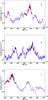Fig. 1 Simulated light curves (blue) with the adaptive-binning light curves superimposed (step 1: black open squares, step 2: red solid circles) for three variable sources. MET stands for mission elapsed time.

Fig. 2 Same as Fig. 1a but the analysis was conducted assuming a reversed arrow of time.

An adverse feature of the method is the flare truncation (the light curve in Fig. 1c shows such a feature at MET ≃ 255 000 000). When a significant flare occurs after a long period of low activity, a non-negligible number of photons from the flare has to be “consumed” to counterbalance the accumulated background photons and enable the criterion to be fulfilled. Possible ways to mitigate this effect are being explored and will be implemented in future versions. The tools allow light curves to be generated by considering either increasing or decreasing photon times, so the robustness of any analysis results (time lags, duty cycles, rise and decay times, etc.) can be tested by using both flavors.

Figure 1c may convey the impression that the adaptive-binning method will lead to light curves lagging the real one. However, cross-correlation analyses have shown that no significant lag is observed for the light curves investigated here, probably because truncation affects only very few bins and the flare leading edges are still well sampled.

Figure 3 shows the distribution of relative flux uncertainties calculated from the pylikelihood analysis for the three variable sources. All three distributions are centered at a value close to the target Δ₀ = 25% (depicted by the dashed line) with essentially all values included in the range 20 − 30% with a typical rms of 3%, demonstrating the performance of the method.

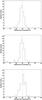Fig. 3 Distribution of relative flux uncertainties given by the pylikelihood analysis for three variable sources. The dashed line depicts the target Δ0 = 25%.

3.3. Comparison with the Bayesian blocks method

The adaptive-binning method bears some resemblance to the Bayesian blocks (BB) method (Scargle 1998; Jackson et al. 2003, 2005). Both methods produce a time binning that adapts itself to the data instead of an arbitrary a priori binning. The main difference is that the BB method gives the optimal segmentation of the data into time intervals during which the data are statistically consistent with a constant flux, whereas in the adaptive-binning method, the segmentation criterion is based on a given value of σ_ln F (or significance) regardless of whether the flux varies within the bin.

Figure 4 shows the results of the BB method applied to the LAT data (Scargle et al., in prep.) for the same simulated light curves as for the adaptive-binning method, for flux above 100 MeV. Photons were selected within a radius of 1.32° around the source. This radius was chosen so that the source differential flux dN/dΩ (spread due to the finite point-spread function, PSF) at maximum radius is equal to the background brightness, leading to a close-to-optimal sensitivity. The BB light curves are plotted in Fig. 4 for false positive rates 0.1%, 1% and 10%; these rates were calibrated via simulations. The dashed curves correspond to the BB results, with an ad hoc correction for the expected constant diffuse background contribution, while the solid curves display the results of the subsequent pylikelihood analysis for the same time intervals. The comparison between Figs. 1 and 4 shows that the adaptive-binning method allows for the study of fainter sources than the BB method, because the adaptive-binning method makes use of the signal/background ratio evaluated with the energy-dependent PSF and models of the diffuse backgrounds while the BB method only considers events lying within the acceptance cone centered on the source position. The two methods are complementary. The BB method is well-suited for detecting the departures from constant-flux behavior in a largely model-independent way, while the adaptive-binning is better for investigating source-specific flux variations in the presence of background sources, which may or may not also be varying. Owing to its better flux sensitivity, the flare rise and decay times as well as the source duty cycle are expected to be determined more accurately with the adaptive-binning method for most of the variable LAT sources. Furthermore, the adaptive-binning method can automatically account for time-dependent spectral variations, whereas the BB method, as applied here, does not.

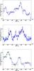Fig. 4 Simulated light curves (blue) with the Bayesian blocks light curves superimposed for false positive rates = 0.1% (red), 1% (green), 10% (black). Some curves are identical. Dashed: BB results, solid: pylikelihood-analysis results for the same time intervals.

3.4. Caveats explored with steady sources

Steady sources with three different fluxes (F₁₀₀ = 0.5, 1 and 5) and two different photon spectral indices (Γ = 2.0 and 2.4) were simulated over the same 11-month long period as for variable sources. Fifty realizations were performed for each case. The average numbers of bins in the light curves as well as the optimum energies are reported in Table 1 for the different cases. For F₁₀₀ = 1 and Γ = 2.0, a light curve where fluxes are estimated after step 1 (i.e., using the simple maximum-likelihood procedure described in the appendix) for a particular realization is compared to that resulting from step 2 (i.e., where fluxes are computed with the whole pylikelihood analyses with the time intervals established in step 1) in Fig. 5. There is a good agreement between these fluxes, which holds for all realizations and parameter sets. Examples of adaptive binning light curves for the flux are shown in Fig. 6 for the different cases, while light curves for the photon spectral index are displayed in Fig. 7. Figure 8 compares the flux distributions obtained via the adaptive- and fixed-binning methods by summing up all realizations. For a given set of conditions, the distributions have similar means and rms but different skews. A positive skew (typically equal to 1σ for the distributions shown in Fig. 8) is a feature of the adaptive-binning method. A positive fluctuation in flux leads to a shorter-than-average bin associated with a high apparent flux. A negative fluctuation has less chance to be recorded since the bin will be extended until enough photons have been accumulated to meet the Δ₀-wise criterion. The photon index distributions have been found to be very similar for the two methods and close to Gaussian distributions.

The distributions of relative statistical uncertainties obtained with the adaptive-binning method (resulting from step 2) are presented in Fig. 9. These distributions are more Gaussian-like than those obtained for variable sources, with a mean value close to 25% as required and a typical rms of about 1.7%. Simulations performed for a very low flux of F₁₀₀ = 0.1 (Γ = 2.0), where the method yields a single bin over the 11-month period, show that the mean of the distribution remains within 10% of the target value even in that extreme case.

The possible biases induced by this method are explored in the following.

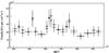Fig. 5 Comparison of flux from the tool, i.e., after step 1 (open diamonds) and flux resulting from the pylikelihood analyses, i.e., after step 2 (filled circles) for a simulated constant source with F100 = 1 and Γ = 2.4.

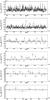Fig. 6 Examples of light curves for the different sets of parameters. From top to bottom: (Γ,F100) = (2.0,5), (2.4, 5), (2.0, 1), (2.4, 1), (2.0, 0.5), (2.4, 0.5). The solid line depicts the true flux value.

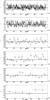Fig. 7 Temporal evolution of the measured photon spectral index. From top to bottom: (Γ,F100) = (2.0,5), (2.4, 5), (2.0, 1), (2.4, 1), (2.0, 0.5), (2.4, 0.5). The solid line depicts the true photon index.

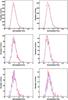Fig. 8 Normalized flux distributions for adaptive (solid) and fixed (dashed) binnings and steady sources with Γ = 2.0 (left) and Γ = 2.4 (right), F100 = 5, 1, 0.5 from top to bottom.

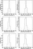Fig. 9 Distribution of σln F for Δ0 = 25% (depicted by a dashed line) for the different parameter sets: Γ = 2.0 (left) and Γ = 2.4 (right), F100 = 5, 1, 0.5 from top to bottom.

3.4.1. Bias and statistical fluctuations in flux and photon-index measurements

The pylikelihood analysis is expected to provide the correct mean flux and photon spectral index over all possible time intervals. We nevertheless checked for the absence of biases in the measurements of these parameters when the time intervals were determined with the present method. Furthermore, possible additional fluctuations in the measured parameters could arise from the intrinsic correlation between bin width and photon contents of the bin. Both effects are addressed here.

One defines ΔF (ΔΓ) as the difference, expressed in sigma, between the measured flux (index) and the average value measured over the whole 11-month period. Summing over all realizations, the distributions of the means (left) and rms (right) of the ΔF (top) and ΔΓ (bottom) distributions are displayed in Fig. 11 for a particular set of parameters. The results of the adaptive- (solid) and fixed- (dashed) binning methods are compared in this figure. The means ⟨ΔF⟩  and ⟨ΔΓ⟩  are listed in Tables 2 and 3 respectively, while the rms values are given in Tables 4 and 5.

A small bias is observed in the mean flux values. Since similar features are seen for both adaptive- and fixed-binning light curves, one can safely conclude that this bias arises from small systematics effects pertaining to our pylikelihood analysis and is not created by the adaptive-binning approach.

The average rms values are found to be close to the expected value of 1 for all cases (with slightly lower values for the adaptive-binning approach relative to the fixed-binning one). One can thus exclude that the adaptive-binning approach gives rise to significant fluctuations in the measured parameters.

3.4.2. Flux-index correlation

Another matter worth investigating is the correlation between measured photon index and flux in a given time interval. All photons do not contribute equally to the fulfillment of the criterion, with higher-energy photons contributing more. The detection of a series of photons with higher-than-average energies will thus lead to the criterion being satisfied faster and consequently to the interval under consideration being closed earlier. To evaluate whether the adaptive-binning method creates additional correlation between the photon spectral index and flux (as measured in step 2), the corresponding correlation factor was computed for each realization. Since E_min was chosen as the optimum energy, for which the correlation between photon index and integral flux is minimum by definition, the observed correlation factor is expected to be small. The correlation-factor distributions obtained for adaptive and fixed binnings are shown in Fig. 10. For all cases, the distributions are very similar for the two approaches and are all centered at low values, with higher fluctuations for lower fluxes. Therefore, the measured photon spectral indices and fluxes do not appear to be more correlated when using an adaptive binning relative to a fixed binning.

3.4.3. Interbin correlation

In the adaptive-binning method, the starting time of a given bin depends on the starting time and flux-dependent width of the previous bin and thus by recurrence on the whole flux history since the start of the light curve. In this section, we explore the impact of the interbin correlation on the measured source parameters by comparing these in two consecutive bins. A comparison will again be made with the results of a similar analysis performed with a fixed binning, for which fluxes measured in consecutive bins are independent by nature. The flux (index) in one bin is plotted versus the flux (index) in the next bin in Fig. 12 left (right) for the whole light curve of a particular realization.

The distribution of correlation factors obtained with the different realizations are presented in Fig. 13. No significant differences are observed between distributions obtained with adaptive and fixed binnings for all cases. Both distributions are centered close to 0 (as expected for the fixed-binning case), demonstrating that the interbin dependence intrinsic to the adaptive binning method has little impact on the correlation between parameters measured in consecutive bins.

4. High-level analysis with variable sources

4.1. Duty cycle

One way to describe variations in a light curve is via a duty cycle, corresponding to the fraction of time a source is in a “bright” state. More generally this can be presented as a flux distribution or its integral, the cumulative distribution function (CDF). In Fig. 14 we have plotted flux, normalized to a mean of 1, versus 1-CDF, for the light curves displayed in Fig. 1. The curves give the fraction of time (1-CDF) that a source is above a particular flux level. Four curves are shown for each light curve, the “true” light curve, the adaptive-binning light curve, the fixed-binning light curve (with the same numbers of bins as the adaptive-binning light curve) and the fixed-binning light curve with higher (16 times) time resolution. The two fixed-binning light curves are complementary in that the high resolution one works well at the high-flux end but fails at the faint end where the noise governs the distribution because of the low signal-to-noise ratio of the individual points. With adaptive binning the bin widths can be optimized such that in the presence of noise, the flux distribution, or duty cycle, can be described over a much wider range than is possible when a fixed bin width is used. The wider the range in fluxes, the more advantageous the adaptive binning for this type of analysis.

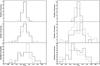Fig. 10 Distributions of correlation factor between spectral index and flux for adaptive (solid) and fixed (dashed) binnings. Γ = 2.0 (left), Γ = 2.4 (right), F100 = 5, 1, 0.5 from top to bottom.

Fig. 11 Distributions of mean values and rms for flux (two top panels) and photon index (two bottom panels) obtained in adaptive- (solid) and fixed-binning (dashed) light curves. In this example, Γ = 2.4 and F100 = 5.

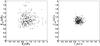Fig. 12 Fluxes (left) and photon spectral indices (right) measured in consecutive bins plotted one against another for a given realization.

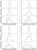Fig. 13 Distributions of correlation factors between consecutive bins both for flux (top panels) and photon spectral index (bottom panels). Γ = 2.0 (left-hand panels) and Γ = 2.4 (right-hand panels), F100 = 5, 1, 0.5 from top to bottom in each panel. Solid: adaptive binning, dashed: fixed binning.

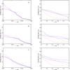Fig. 14 Normalized flux is plotted against the parameter 1-CDF, obtained for the different light curves shown in Fig. 1. Left: whole range, right: zoom on the low-CDF region. Solid purple: true light curve, dashed green: fixed binning, dotted red: fixed binning with higher resolution, dot-dashed blue: adaptive binning.

4.2. Power density spectrum (PDS)

The PDS is one of the main tools used to characterize light curve variability. For evenly sampled data the PDS is computed directly via the Fourier transform of the light curve. For light curves with uneven sampling the Lomb-Scargle algorithm can be used and the PDS distortions caused by the sampling are usually modeled by comparison with simulated light curves (Done et al. 1992; Uttley et al. 2002). This method cannot easily be applied to adaptively binned light curves since the bin widths depend on flux, making time sampling different for each simulation. It is still possible to qualitatively estimate the PDS for an adaptive-binning light curve. To do this we oversampled the light curve with a linear interpolation between the center of each of the adaptive time bins. The PDS was then computed with a standard Fourier transform. The binning and interpolation modify the power density around and above the frequencies corresponding to the widths of the time bins. To check at what frequencies this becomes important for a particular light curve, we computed the distribution of Nyquist frequencies (equal to 0.5/dt where dt is the bin width) associated with the bin widths. In Fig. 15 this distribution is plotted for the three simulated light curves shown in Fig. 1, in each case together with the PDS for the adaptive- and fixed-binning light curves as well as for the true light curve. For the fixed-binning case we also show the PDS after subtraction of the white noise level, illustrating where, for this PDS, the signal is lost in the noise. It is clear from these examples that the PDS of the adaptive-binning light curve provides a qualitatively reasonable estimate of the PDS over a similar frequency range as the PDS for the fixed binning case. At the higher frequencies, however, the adaptive-binning PDS, as we computed it here, is determined essentially by the binning interpolation. A more detailed discussion of the PDS properties and ways in which the binning effects can be taken into account is beyond the scope of the present paper.

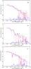Fig. 15 Comparison of power density spectra for the same simulations as in Fig. 1. In each plot the solid curve (purple) is the PDS of the true light curve. The dashed (green) and long dashed (red) curves are the PDS calculated for the fixed binned light curves, the white noise level being subtracted for the latter. The PDS of the adaptive binned light curve is plotted as a dash-dot curve. All PDS curves were smoothed by averaging over logarithmic frequency bins. The distribution of Nyquist frequencies corresponding to the time widths of the adaptive bins is shown by the histogram (blue). Note that this distribution is plotted in linear scale, the zero level corresponding to the lower limit of the vertical axis.

5. Summary

We have presented a method enabling constant-uncertainty/ constant-significance light curves to be computed with the Fermi-LAT data. These light curves encapsulate more information than do fixed-binning light curves, without favoring any a priori arbitrary timescale and while avoiding upper limits. Although primarily developed for blazar studies, the method is applicable to all variable sources. The current implementation allows the time intervals to be calculated in a simple and quick way, while the reported parameters result from the standard LAT analysis. A slight skew in the measured flux distribution is a feature of the method. Possible adverse effects were explored by Monte-Carlo simulations but no significant problems have been revealed. This method opens capabilities regarding timing analysis in the γ-ray domain that were only available so far at longer wavelengths.

Acknowledgments

It is a pleasure to thank J. Chiang, S. Fegan and J. Scargle for useful discussions and suggestions. The Fermi-LAT Collaboration acknowledges generous ongoing support from a number of agencies and institutes that have supported both the development and the operation of the LAT and the scientific data analysis. These include the National Aeronautics and Space Administration and the Department of Energy in the United States, the Commissariat à l’Énergie Atomique and the Centre National de la Recherche Scientifique/Institut National de Physique Nucléaire et de Physique des Particules in France, the Agenzia Spaziale Italiana and the Istituto Nazionale di Fisica Nucleare in Italy, the Ministry of Education, Culture, Sports, Science and Technology (MEXT), High Energy Accelerator Research Organization (KEK) and Japan Aerospace Exploration Agency (JAXA) in Japan, and the K. A. Wallenberg Foundation, the Swedish Research Council and the Swedish National Space Board in Sweden. Additional support for science analysis during the operations phase is gratefully acknowledged from the Istituto Nazionale di Astrofisica in Italy and the Centre National d’Études Spatiales in France.

References

Appendix A: Appendix A

The goal is to estimate the relative integral-flux uncertainty σ_ln F from the data given particular source and background models. Both flux and σ_ln F estimates are based on an unbinned maximum-likelihood method presented in the following. These estimates have been found to agree with those given by the pylikelihood analysis within a few percent. Some of the formulae derived below can also be found in the appendix of Abdo et al. (2010a).

A.1. Log likelihood

The likelihood ℒ is the probability of obtaining the data given an input model that is in this case the distribution of the γ-ray fluxes over the sky. The maximum likelihood method consists in maximizing ℒ over the parameter phase space of the model to obtain the best match between the model and the data. Following Cash (1979, Eq. (7)), the logarithm of the likelihood is obtained by adding up the contribution of each photon, with index i in the following, within a region of interest (ROI) over a time interval [T₀,T₁] : $\begin{array}{ccc}\ln \mathrm{ℒ}\mathrm{=}\sum _{\mathit{i}}\ln {\mathit{M}}_{\mathit{i}}\mathrm{-}{\mathit{N}}_{\mathrm{pred}}\mathit{,}& & \end{array}$(A.1)where M_i = Exp(E_i,T₀,T₁) [S_s(E_i)PSF(r_i,E_i) + S_B(E_i)]  is the model event density, E_i is the photon energy, r_i is the angular deviation from the source position, Exp(E_i,T₀,T₁) is the exposure (time ×  effective area) over the considered time period, S_s(E_i) is the differential source spectrum, assumed to be a power law in the following, $\begin{array}{ccc}{\mathit{S}}_{\mathrm{s}}\mathrm{(}{\mathit{E}}_{\mathit{i}}\mathrm{)}\mathrm{=}\mathit{A}{\left(\frac{{\mathit{E}}_{\mathit{i}}}{{\mathit{E}}_{\mathrm{0}}}\right)}^{\mathrm{-}\mathrm{\Gamma }}\mathit{,}& & \end{array}$(A.2)where E₀ is a reference energy, A is the differential flux for E_i = E₀ and Γ is the photon spectral index, PSF(r_i,E_i) is the point-spread function⁵, S_B(E_i) is the differential background per solid angle unit. Finally, $\begin{array}{ccc}{\mathit{N}}_{\mathrm{pred}}\mathrm{=}\mathrm{\int }\mathit{Exp}\mathrm{(}\mathit{E,}{\mathit{T}}_{\mathrm{0}}\mathit{,}{\mathit{T}}_{\mathrm{1}}\mathrm{)}\left[{\mathit{S}}_{\mathrm{s}}\mathrm{\left(}\mathit{E}\mathrm{\right)}\mathrm{+}\mathrm{\int }{\mathit{S}}_{\mathit{B}}\mathrm{\left(}\mathit{E}\mathrm{\right)}\mathrm{d\Omega }\right]\mathrm{d}\mathit{E}& & \end{array}$(A.3)is the number of photons within the ROI predicted by the model.

A.2. Significance/flux calculation

The difference between lnℒ assuming that the source is present or absent is: $\begin{array}{ccc}\mathrm{\Delta }\ln \mathrm{ℒ}\mathrm{=}\sum _{\mathit{i}}\ln \left[\mathrm{1}\mathrm{+}\mathit{g}\mathrm{(}{\mathit{r}}_{\mathit{i}}\mathit{,}{\mathit{E}}_{\mathit{i}}\mathrm{)}\right]\mathrm{-}{\mathit{N}}_{\mathrm{src}}\mathit{,}& & \end{array}$(A.4)where g(r_i,E_i) is the local source/background ratio $\begin{array}{ccc}\mathit{g}\mathrm{(}{\mathit{r}}_{\mathit{i}}\mathit{,}{\mathit{E}}_{\mathit{i}}\mathrm{)}\mathrm{=}\frac{{\mathit{S}}_{\mathrm{s}}\mathrm{(}{\mathit{E}}_{\mathit{i}}\mathrm{)}\mathit{PSF}\mathrm{(}{\mathit{r}}_{\mathit{i}}\mathit{,}{\mathit{E}}_{\mathit{i}}\mathrm{)}}{{\mathit{S}}_{\mathit{B}}\mathrm{(}{\mathit{E}}_{\mathit{i}}\mathrm{)}}& & \end{array}$(A.5)and N_src is the predicted number of photons coming from the source only: $\begin{array}{ccc}{\mathit{N}}_{\mathrm{src}}\mathrm{=}\mathrm{\int }\mathit{Exp}\mathrm{(}\mathit{E,}{\mathit{T}}_{\mathrm{0}}\mathit{,}{\mathit{T}}_{\mathrm{1}}\mathrm{)}{\mathit{S}}_{\mathrm{S}}\mathrm{\left(}\mathit{E}\mathrm{\right)}\mathrm{d}\mathit{E}\mathit{.}& & \end{array}$(A.6)The flux of the source is estimated by maximizing Δlnℒ with respect to A (Γ is usually set fixed in step 1).

The test statistic (TS) is defined as 2Δlnℒ. In principle, TS behaves as a χ² distribution with a number of degrees of freedom equal to the number of free source parameters, but in our particular case the statistic is modified because negative flux values are not allowed in the fit (“1/2 χ²”). For a sufficiently large N_σ one has: $\mathit{TS}\mathrm{\simeq }{\mathit{N}}_{\mathit{\sigma }}^{\mathrm{2}}$. The TS of the source is the sum of the contribution of each photon within the ROI with a weight depending on r_i. As long as the ROI radius is large enough to include all photons from the source, the TS computed over the ROI is independent of the ROI size. Indeed, the contributions from distant photons are negligible because there are suppressed by the point-spread function.

A.3. Relative flux uncertainty

The relative flux uncertainty σ_ln F is calculated in step 1 using the formulae below to consistently estimate σ_ln F as obtained in step 2. These formulae are derived under the assumption that Γ is left free in the fit performed in step 2 (otherwise, one would just have ${\mathit{\sigma }}_{\ln \hspace{0.17em}\mathit{F}}\mathrm{=}\frac{\mathrm{\Delta }\mathit{A}}{\mathit{A}}$).

The elements of the Hessian matrix, the inverse of the covariance matrix, can be calculated as $\begin{array}{ccc}{\mathit{H}}_{{\mathit{x}}_{\mathrm{1}}{\mathit{x}}_{\mathrm{2}}}\mathrm{\equiv }\frac{{\mathit{\partial }}^{\mathrm{2}}\ln \mathrm{ℒ}}{\mathit{\partial }{\mathit{x}}_{\mathrm{1}}\mathit{\partial }{\mathit{x}}_{\mathrm{2}}}\mathrm{=}\frac{{\mathit{\partial }}^{\mathrm{2}}\mathrm{\Delta }\ln \mathrm{ℒ}}{\mathit{\partial }{\mathit{x}}_{\mathrm{1}}\mathit{\partial }{\mathit{x}}_{\mathrm{2}}}\mathit{,}& & \end{array}$(A.7)where the parameters x_1,2 are either A or Γ.

The relative statistical uncertainty on the differential flux is $\begin{array}{ccc}\frac{\mathrm{\Delta }\mathit{A}}{\mathit{A}}\mathrm{=}\frac{{\left|{\mathit{H}}_{\mathit{AA}}\right|}^{\mathrm{-}\mathrm{1}\mathit{/}\mathrm{2}}}{\mathit{A}}\mathrm{=}{\left[\sum _{\mathit{i}}\frac{\mathit{g}{\mathrm{(}{\mathit{r}}_{\mathit{i}}\mathit{,}{\mathit{E}}_{\mathit{i}}\mathrm{)}}^{\mathrm{2}}}{{\left(\mathrm{1}\mathrm{+}\mathit{g}\mathrm{(}{\mathit{r}}_{\mathit{i}}\mathit{,}{\mathit{E}}_{\mathit{i}}\mathrm{)}\right)}^{\mathrm{2}}}\right]}^{\mathrm{-}\mathrm{1}\mathit{/}\mathrm{2}}\mathrm{·}& & \end{array}$(A.8)The cross-term element H_AΓ is $\begin{array}{ccc}{\mathit{H}}_{\mathit{A}\mathrm{\Gamma }}\mathrm{=}\mathrm{-}\frac{\mathrm{1}}{\mathit{A}}\sum _{\mathit{i}}\frac{\mathit{g}\mathrm{(}{\mathit{r}}_{\mathit{i}}\mathit{,}{\mathit{E}}_{\mathit{i}}\mathrm{)}\ln \mathrm{(}{\mathit{E}}_{\mathit{i}}\mathit{/}{\mathit{E}}_{\mathrm{0}}\mathrm{)}}{{\left(\mathrm{1}\mathrm{+}\mathit{g}\mathrm{(}{\mathit{r}}_{\mathit{i}}\mathit{,}{\mathit{E}}_{\mathit{i}}\mathrm{)}\right)}^{\mathrm{2}}}& & \\ \mathrm{+}\frac{\mathrm{1}}{\mathit{A}}”\mathit{Exp}\mathrm{(}\mathit{E,}{\mathit{T}}_{\mathrm{0}}\mathit{,}{\mathit{T}}_{\mathrm{1}}\mathrm{)}{\mathit{S}}_{\mathrm{S}}\mathrm{\left(}\mathit{E}\mathrm{\right)}\mathit{PSF}\mathrm{\left(}\mathit{r,E}\mathrm{\right)}\ln \mathrm{(}\mathit{E}\mathit{/}{\mathit{E}}_{\mathrm{0}}\mathrm{)}\mathrm{d\Omega d}\mathit{E}\mathit{.}& & \end{array}$(A.9)On average (over many observations of the same source), H_AΓ can be written as 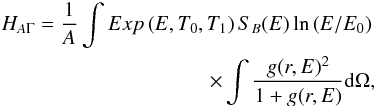$\begin{array}{ccc}{\mathit{H}}_{\mathit{A}\mathrm{\Gamma }}\mathrm{=}\frac{\mathrm{1}}{\mathit{A}}\mathrm{\int }\mathit{Exp}\mathrm{(}\mathit{E,}{\mathit{T}}_{\mathrm{0}}\mathit{,}{\mathit{T}}_{\mathrm{1}}\mathrm{)}{\mathit{S}}_{\mathit{B}}\mathrm{\left(}\mathit{E}\mathrm{\right)}\ln \mathrm{(}\mathit{E}\mathit{/}{\mathit{E}}_{\mathrm{0}}\mathrm{)}& & \\ \mathrm{\times }\mathrm{\int }\frac{\mathit{g}\mathrm{(}\mathit{r,E}{\mathrm{)}}^{\mathrm{2}}}{\mathrm{1}\mathrm{+}\mathit{g}\mathrm{\left(}\mathit{r,E}\mathrm{\right)}}\mathrm{d\Omega }\mathit{,}& & \end{array}$(A.10)assuming that the model is correct, i.e., the actual photon energy distributions are given by S_S(E) and S_B(E) for the source and background, respectively. Defining the pivot energy E_pivot as the value of the reference energy E₀ (Eq. (A.2)) for which H_AΓ = 0, one obtains 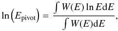$\begin{array}{ccc}\ln \mathrm{(}{\mathit{E}}_{\mathrm{pivot}}\mathrm{)}\mathrm{=}\frac{\mathrm{\int }\mathit{W}\mathrm{\left(}\mathit{E}\mathrm{\right)}\ln \mathit{E}\mathrm{d}\mathit{E}}{\mathrm{\int }\mathit{W}\mathrm{\left(}\mathit{E}\mathrm{\right)}\mathrm{d}\mathit{E}}\mathit{,}& & \end{array}$(A.11)where 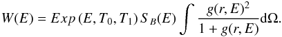$\begin{array}{ccc}\mathit{W}\mathrm{\left(}\mathit{E}\mathrm{\right)}\mathrm{=}\mathit{Exp}\mathrm{(}\mathit{E,}{\mathit{T}}_{\mathrm{0}}\mathit{,}{\mathit{T}}_{\mathrm{1}}\mathrm{)}{\mathit{S}}_{\mathit{B}}\mathrm{\left(}\mathit{E}\mathrm{\right)}\mathrm{\int }\frac{\mathit{g}\mathrm{(}\mathit{r,E}{\mathrm{)}}^{\mathrm{2}}}{\mathrm{1}\mathrm{+}\mathit{g}\mathrm{\left(}\mathit{r,E}\mathrm{\right)}}\mathrm{d\Omega }\mathit{.}& & \end{array}$(A.12)In the following, the reference energy E₀ is set to E_pivot, as ΔA/A is minimum in that case. The Hessian matrix is then diagonal and thus so is the covariance matrix.

F is the integral flux between E_min and + ∞. It can be written as 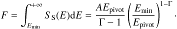$\begin{array}{ccc}\mathit{F}\mathrm{=}{\mathrm{\int }}_{{\mathit{E}}_{\min }}^{\mathrm{+}\mathrm{\infty }}{\mathit{S}}_{\mathrm{S}}\mathrm{\left(}\mathit{E}\mathrm{\right)}\mathrm{d}\mathit{E}\mathrm{=}\frac{\mathit{A}{\mathit{E}}_{\mathrm{pivot}}}{\mathrm{\Gamma }\mathrm{-}\mathrm{1}}{\left(\frac{{\mathit{E}}_{\min }}{{\mathit{E}}_{\mathrm{pivot}}}\right)}^{\mathrm{1}\mathrm{-}\mathrm{\Gamma }}\mathrm{·}& & \end{array}$(A.13)The relative uncertainty of F, σ_ln F, is obtained by propagating the errors of A and Γ, making use of the fact that the covariance matrix is diagonal for this choice of E₀: $\begin{array}{ccc}{\mathit{\sigma }}_{\ln \hspace{0.17em}\mathit{F}}\mathrm{=}{\left[{\left(\frac{\mathrm{\Delta }\mathit{A}}{\mathit{A}}\right)}^{\mathrm{2}}\mathrm{+}{\mathit{\sigma }}_{\mathrm{\Gamma }}^{\mathrm{2}}{\left(\ln \left(\frac{{\mathit{E}}_{\min }}{{\mathit{E}}_{\mathrm{pivot}}}\right)\mathrm{+}\frac{\mathrm{1}}{\mathrm{\Gamma }\mathrm{-}\mathrm{1}}\right)}^{\mathrm{2}}\right]}^{\mathrm{1}\mathit{/}\mathrm{2}}\mathit{,}& & \end{array}$(A.14)where σ_Γ is the uncertainty of Γ, σ_Γ = | H_γγ |  ^− 1/2.

A.4. Optimum energy

Using the optimum energy E₁, corresponding to the energy for which the second term in Eq. (A.14) cancels, for E_min will lead to the minimum σ_ln F relative to other choices of E_min: $\begin{array}{ccc}\ln {\mathit{E}}_{\mathrm{1}}\mathrm{=}\ln {\mathit{E}}_{\mathrm{pivot}}\mathrm{-}\frac{\mathrm{1}}{\mathrm{\Gamma }\mathrm{-}\mathrm{1}}\mathrm{·}& & \end{array}$(A.15)In that case σ_ln F is equal to ΔA/A and is obtained from Eq. (A.8).

All Tables

All Figures

	Fig. 1 Simulated light curves (blue) with the adaptive-binning light curves superimposed (step 1: black open squares, step 2: red solid circles) for three variable sources. MET stands for mission elapsed time.
In the text

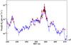	Fig. 2 Same as Fig. 1a but the analysis was conducted assuming a reversed arrow of time.
In the text

	Fig. 3 Distribution of relative flux uncertainties given by the pylikelihood analysis for three variable sources. The dashed line depicts the target Δ0 = 25%.
In the text

	Fig. 4 Simulated light curves (blue) with the Bayesian blocks light curves superimposed for false positive rates = 0.1% (red), 1% (green), 10% (black). Some curves are identical. Dashed: BB results, solid: pylikelihood-analysis results for the same time intervals.
In the text

	Fig. 5 Comparison of flux from the tool, i.e., after step 1 (open diamonds) and flux resulting from the pylikelihood analyses, i.e., after step 2 (filled circles) for a simulated constant source with F100 = 1 and Γ = 2.4.
In the text

	Fig. 6 Examples of light curves for the different sets of parameters. From top to bottom: (Γ,F100) = (2.0,5), (2.4, 5), (2.0, 1), (2.4, 1), (2.0, 0.5), (2.4, 0.5). The solid line depicts the true flux value.
In the text

	Fig. 7 Temporal evolution of the measured photon spectral index. From top to bottom: (Γ,F100) = (2.0,5), (2.4, 5), (2.0, 1), (2.4, 1), (2.0, 0.5), (2.4, 0.5). The solid line depicts the true photon index.
In the text

	Fig. 8 Normalized flux distributions for adaptive (solid) and fixed (dashed) binnings and steady sources with Γ = 2.0 (left) and Γ = 2.4 (right), F100 = 5, 1, 0.5 from top to bottom.
In the text

	Fig. 9 Distribution of σln F for Δ0 = 25% (depicted by a dashed line) for the different parameter sets: Γ = 2.0 (left) and Γ = 2.4 (right), F100 = 5, 1, 0.5 from top to bottom.
In the text

	Fig. 10 Distributions of correlation factor between spectral index and flux for adaptive (solid) and fixed (dashed) binnings. Γ = 2.0 (left), Γ = 2.4 (right), F100 = 5, 1, 0.5 from top to bottom.
In the text

	Fig. 11 Distributions of mean values and rms for flux (two top panels) and photon index (two bottom panels) obtained in adaptive- (solid) and fixed-binning (dashed) light curves. In this example, Γ = 2.4 and F100 = 5.
In the text

	Fig. 12 Fluxes (left) and photon spectral indices (right) measured in consecutive bins plotted one against another for a given realization.
In the text

	Fig. 13 Distributions of correlation factors between consecutive bins both for flux (top panels) and photon spectral index (bottom panels). Γ = 2.0 (left-hand panels) and Γ = 2.4 (right-hand panels), F100 = 5, 1, 0.5 from top to bottom in each panel. Solid: adaptive binning, dashed: fixed binning.
In the text

	Fig. 14 Normalized flux is plotted against the parameter 1-CDF, obtained for the different light curves shown in Fig. 1. Left: whole range, right: zoom on the low-CDF region. Solid purple: true light curve, dashed green: fixed binning, dotted red: fixed binning with higher resolution, dot-dashed blue: adaptive binning.
In the text

Fig. 15 Comparison of power density spectra for the same simulations as in Fig. 1. In each plot the solid curve (purple) is the PDS of the true light curve. The dashed (green) and long dashed (red) curves are the PDS calculated for the fixed binned light curves, the white noise level being subtracted for the latter. The PDS of the adaptive binned light curve is plotted as a dash-dot curve. All PDS curves were smoothed by averaging over logarithmic frequency bins. The distribution of Nyquist frequencies corresponding to the time widths of the adaptive bins is shown by the histogram (blue). Note that this distribution is plotted in linear scale, the zero level corresponding to the lower limit of the vertical axis.

In the text

References

- Abdo, A. A., Ackermann, M., Ajello, M., et al. 2010a, ApJS, 188, 405 [NASA ADS] [CrossRef] [Google Scholar]
- Abdo, A. A., Ackermann, M., Ajello, M., et al. 2010b, ApJ, 710, 1271 [NASA ADS] [CrossRef] [Google Scholar]
- Abdo, A. A., Ackermann, M., Ajello, M., et al. 2011, Science, 331, 739 [NASA ADS] [CrossRef] [PubMed] [Google Scholar]
- Ackermann, M., Ajello, M., Allafort, A., et al. 2011, ApJ, 743, 171 [NASA ADS] [CrossRef] [Google Scholar]
- Cash, W. 1979, ApJ, 228, 939 [NASA ADS] [CrossRef] [Google Scholar]
- Done, C., Madejski, G. M., Mushotzky, R. F., et al. 1992, ApJ, 400, 138 [NASA ADS] [CrossRef] [Google Scholar]
- Jackson, B., Scargle, J. D., Barnes, D., et al. 2003 [arXiv:astro-ph/0309285] [Google Scholar]
- Jackson, B., Scargle, J. D., Barnes, D., et al. 2005, IEEE Signal Processing Letters, 12, 105 [NASA ADS] [CrossRef] [Google Scholar]
- Scargle, J. D. 1998, ApJ, 504, 405 [NASA ADS] [CrossRef] [Google Scholar]
- Uttley, P., McHardy, I. M., & Papadakis, I. E. 2002, MNRAS, 332, 231 [NASA ADS] [CrossRef] [Google Scholar]