| Issue |
A&A
Volume 544, August 2012
|
|
|---|---|---|
| Article Number | A25 | |
| Number of page(s) | 21 | |
| Section | Catalogs and data | |
| DOI | https://doi.org/10.1051/0004-6361/201118506 | |
| Published online | 23 July 2012 | |
Multifrequency study of GHz-peaked spectrum sources and candidates with the RATAN-600 radio telescope
1
Special Astrophysical Observatory of RAS, 369167
Nizhnij Arkhyz,
Russia
e-mail: This email address is being protected from spambots. You need JavaScript enabled to view it.
2
Kazan Federal University, 18 Kremlyovskaya St., 420008
Kazan,
Russia
3
Aalto University, Metsähovi Radio Observatory,
Metsähovintie 114, 02540
Kylmälä,
Finland
Received:
23
November
2011
Accepted:
11
May
2012
Abstract
Context. Gigahertz peaked spectrum (GPS) radio sources are a class of extragalactic radio sources characterized by a spectral peak in the gigahertz domain. They are a mixed class of quasars and galaxies. A large proportion of the sources studied in the literature have only few data points in the radio domain, and the determination of variability and shape of the simultaneous spectra is inadequate. Sources currently included in the GPS source lists are very heterogeneous.
Aims. We present the observational results from 12 observing campaigns (carried out between 2006 and 2010) at the RATAN-600 radio telescope to obtain the simultaneous radio spectra, which is valuable and necessary to derive genuine GPS sources from flat-spectrum radio sources caught in a flaring state when their spectra are temporarily inverted. The sample contains both quasar- and galaxy-type GPS (122 sources) identified in the literature.
Methods. The observations were carried out at six frequencies (1.1, 2.3, 4.8, 7.7, 11.2 and 21.7 GHz). The flux densities were measured at several epochs. A six-frequency broadband radio spectrum was obtained by observing simultaneously with an accuracy of up to a minute at 1.4, 2.7, 3.9, 6.25, 13, and 30 cm.
Results. The original GPS source samples were highly contaminated. Finally, we selected 29% GPS source candidates within the sample. We found some difference in spectral properties between GPS galaxies and quasars within the sample. The GPS galaxies demonstrate a steeper spectral index in the optically thin part of the spectra. There are only relatively few (17) sources whose radio spectra strictly agree with the spectra of homogeneous self-absorbed synchrotron sources. The narrowest radio spectra are found in both ultra-high-z (z ≥ 1.8) and low-z (0.02 ≤ z ≤ 0.7, FWHM ~ 0.9) convex spectrum radio sources. The majority of quasars within this sample should be considered as flat-spectrum radio sources with a temporarily inverted spectrum, and not as genuine GPS sources. The number of truly convex-spectrum sources remains low, and the lists of GPS sources should accordingly be revised.
Key words: galaxies: active / galaxies: general / radio continuum: galaxies
© ESO, 2012
1. Introduction
Gigahertz peaked spectrum (GPS) radio sources are a class of extragalactic radio sources characterized by a spectral peak in the gigahertz domain (Spoelstra et al. 1985; O’Dea et al. 1991; O’Dea 1998). They are a mixed class of quasars and galaxies. The mechanism that produces the absorption in the optically thick part in these compact luminous objects is still somewhat unclear. It is commonly believed to be due to synchrotron self-absorption caused by the high density of synchrotron-emitting electrons in the radio source (Snellen et al. 1998), but free-free absorption (FFA) has also been suggested to be able to produce the turnover at GHz frequencies as well as the peak frequency vs. size – anticorrelation observed in many of these sources (Bicknell et al. 1997).
The GPS sources are powerful (log P1.4 ≥ 25 WHz-1), compact (≤1 kpc), and have a convex radio spectrum that peaks between 500 MHz and 10 GHz (in the observer frame). These radio sources make up a significant fraction of the bright (centimeter-wavelength-selected) radio source population (~10%) but they are not well understood. It has been suggested that they are young radio sources (≤104 yr) that evolve into large radio sources (Fanti et al. 1995; Readhead et al. 1996; O’Dea et al. 1991), and studying them would then provide us with important information on early stages of radio source evolution. Alternatively, GPS sources may be compact because a particularly dense environment prevents them from growing larger (O’Dea 1990; Gopal-Krishna & Wiita 1991). Baum et al. (1990) detected faint emission around a GPS source candidate and suggested that the activity could be recurrent: retriggered jets have just started to grow while the relics of earlier jets and lobes are fading away. Whatever is the case, studying GPS sources can help us to understand the origin and nature of active galactic nuclei.
Stanghellini et al. (1990) noticed that the shape of the spectrum distinguishes GPS sources from “normal” compact radio sources. First of all, it has very steep spectral indices, both at the high and at the low frequencies (less than −0.8, and for S ~ να). GPS sources have a lower variability in the total flux density and small fractional polarization when compared to flat-spectrum radio sources (Pearson & Readhead 1988; O’Dea 1990). Usually the low level of polarization for GPS sources (Rudnick & Jones 1982; Pearson & Readhead 1988; O’Dea 1990) and the high Faraday rotation measure (Rudnick & Jones 1982) are connected with a dense environment around GPS (Stanghellini et al. 1990).
A large proportion of quasar-type GPS sources are really not genuine GPS sources, but flat-spectrum radio sources caught in a flaring state when their spectra are temporarily inverted (Torniainen et al. 2005). Most of the remaining genuine GPS sources of mostly quasars exhibit fair variability. The inclusion of blazars and other variable flat-spectrum sources contaminates the GPS source lists and easily leads to an incorrect interpretation of the source properties. The best tool for revealing true GPS-type spectra are long-term observations carried out simultaneously at several frequencies. A large proportion of the sources studied in the literature have only few data points in the radio domain, and the determination of variability and shape of the simultaneous spectra is inadequate. Sources currently included in the GPS source lists are very heterogeneous. It was shown (Tornikoski et al. 2009) that long time-series are more important than very dense sampling, and that even three to five years of data may not be enough for revealing the “typical behaviour” of a source. With short data sets incorrect conclusions are easily drawn about the variability, the shape of the continuum spectrum, the SED (spectral energy distribution), the detection probability at high frequencies, and so on. This leads to misinterpretation of source types and subtypes in samples severely contaminated by incorrectly classified sources.
In this paper we present observational results from 12 observing campaigns (carried out between 2006 and 2010) at the RATAN-600 radio telescope to obtain the simultaneous radio spectra, which are valuable and necessary to derive genuine GPS sources from flat-spectrum radio sources that were caught in a flaring state when their spectra are temporarily inverted. The sample contains both quasar- and galaxy-type GPS (122 sources) identified in the literature. The observations were carried out at six frequencies (1.1, 2.3, 4.8, 7.7, 11.2, and 21.7 GHz).
2. Sample and observations
We have collected a sample of both quasar- and galaxy-type GPS sources identified in the literature. A large proportion of the sources have only few data points in radio, some of the sources have not been monitored for a long time and the determination of the variability and the shape of the simultaneous spectra is inadequate. The sample contains 76 quasar-type and 29 galaxy-type GPS sources and candidates from the literature. The remaining 17 sources were not identified in the optical domain. The list of 122 sources and their characteristics are presented in Table 2.
The observations of GPS sources and candidates were carried out at the RATAN-600 during 12 observing campaigns: July and October 2006, March and April 2007, September 2007, April and June 2008, November and October 2008, April, October and November 2009, January, April, May, and July 2010. The list of observations contains sources accessible either only to the northern sector (declination range from −40° to +49°) or only to the southern sector (declination range from +49° to +84°) of RATAN-600 (total number of sources is 122). The northern and southern sector of the antenna were used. The mode of the meridian instrument was used – the passage of a source through a fixed beam in the upper culmination for objects accessible to the northern sector and in the lower transit for objects accessible to the southern sector. Every source was observed from 3 to 15 times to increase the reliability of results and because of weather conditions.
We processed our observations using modules of the FADPS (Flexible Astronomical Data Processing System) standard reduction package by Verkhodanov (1997) in a Linux environment; this is a reduction system for data from the broadband continuum radiometers of the RATAN-600 secondary mirror. Scans of all sources were corrected for baseline slope when fitted to a Gaussian response. The accuracy of the antenna temperature of each source was determined as the standard error of the mean from N observations of a set, taking into account the Student factor. Details on observation and analysis technique are given by Mingaliev et al. (2001, 2007). The errors of the antenna temperature depend not only on the receiver noise, but also on the atmospheric fluctuations on the scale of the main beam, on the accuracy of antenna surface setting for the actual source observation and on the accuracy of the feed cabin positioning (the cabin with secondary mirror and receivers). The total fractional error in the flux densities is the quadratic sum of the total calibration error and the error in the antenna temperature measurement:  (1)where
-
σt –
total standard error;
-
σc –
standard error of calibration;
-
σm –
standard error of Tant, ν measurement;
-
Sν –
flux density;
-
gν(e) = 1/fν(e)
–
elevation calibration function;
-
Tant, ν – antenna temperature.
The following twelve flux density calibrators were applied to obtain the calibration curve for the northern and southern sector of RATAN-600: J0137+33 (3C48), J0240−23, J0410+76, J0521+16 (3C138), J0542+49 (3C147), J0627−05 (3C161), J1154−35, J1331+30 (3C286), J1347+12, J1411+52 (3C295), J1459+71 (3C309.1), and J2107+42 (NGC7027) (exluding 31 cm calibration). The sources J0240−23, J1154−35 and J0521+16 are the traditional RATAN-600 flux density calibrators at low elevations, and the source J0410+76 – at high declination. Measurements of some calibrators were corrected on angular size and linear polarization, following the data in Ott et al. (1994) and Tabara & Inoue (1980), respectively. The calibration curves (Fig. 1) essentially represent observing-run averages of the combined dependence of the atmospheric-extinction instability and the effective area on the elevation h at the corresponding wavelengths (in the presence of real aberrations owing to the transverse distance of the primary feeds from the electrical axis of the antenna).
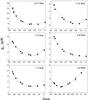 |
Fig. 1 Flux density calibration factor gν versus focus; where focus is the distance from antenna to the secondary mirror compared to the radius of RATAN-600 (it depends on the antenna elevation) at all wavelengths for the northern sector. All data shown for 9 calibrators were averaged during one observational set in 2007. |
3. Flux densities and radio continuum spectra
The flux densities of 122 sources for several epochs with available RATAN-600 observations are given in Table 2.
Column 1 – source name [hhmmss+ddmmss] from the NVSS catalogue;
Col. 2 – optical identifications and redshifts. Information about the optical identification and redshift was taken from the NASA/IPAC Extragalactic database (NED). The abbreviations used are “Q” for quasars, “G” for galaxies, “–” for radio sources with no identification.
Column 3 – RATAN-600 spectrum classification: max = spectrum with maximum in the RATAN-600 frequency range; max1 = possible spectrum with a maximum in low frequencies not accessible to RATAN-600; max2 = variable spectrum with maximum of VarΔS > 2.5 at 21−4.8 GHz; f = flat spectrum (0 ≥ α ≥ −0.5); ris = rising spectrum (α > 0); s = steep spectrum (spectral index α ≤ −0.5); c = complex spectrum (one or more minima);
Col. 4 – observation epochs at RATAN-600 [yyyy.mm];
Col. 5–15 – flux densities and their uncertainties for the corresponding frequencies, including the uncertainty in the source’s antenna temperature and the calibration curve.
Averaged instantaneous spectra at several epochs are shown in Fig. 5. Almost all sources have complete data at all frequencies. Absence of data for some sources at some frequencies is a result of data exclusion because of the following reasons: partial resolution of a source at some frequencies, a source is too weak to be measured reliably, a strong influence of man-made interferences (usually at 31 and 13 cm), strong interferences from the geostationary satellites at 2.7 cm (in declinations between −10° and 0°). Nevertheless, in some cases the data were not excluded in spite of the increase in errors. The values of the standard error of fluxes are: 5−10% for 11.2, 7.7 and 4.8 GHz, 7−20% for 2.3, 1.0 and 21.7 GHz.
We found that 69 sources have a convex spectral shape. But 13 sources of them show considerable variability – the variability index VarΔS > 25% at 21.7−4.8 GHz. The obtained proposed spectral classes for sources under investigation are presented in Table 1. Therefore less than half of the sources of the sample closely follow the typical shape of a GPS source spectrum. The shape of the spectra remained clearly convex for only a fraction of sources of the sample. Most of the sources are variable flat-spectrum sources with the inverted spectral shape only during flares.
Proposed source classes of the sample.
We summarise the variability and spectral properties of the objects with spectral maximum (Table 3). Table 3 lists all the 69 sources for which a spectral maximum could be defined. Column (1) is the name of source; (2) optical classification; (3) indication of GPS and candidates; (4) redshift; (5) is the peak frequency [MHz] in the observer frame; (6) and (7) are the spectral indices of optically thick αbelow and thin αabove parts of spectra and their estimated RMS error; (8) is the value of FWHM in decades of frequency; (9)−(12) is the value of VarS at 4.8, 7.7, 11.2 and 21.7 GHz. The spectral index α is used to describe the slope of a spectrum. It can be calculated by  (2)where S1 is the flux density at the frequency ν1, and S2 the flux density at the frequency ν2. Thus, we define the spectral index α such that S ∝ να. The peak frequency and FWHM parameters of spectra were determined from the fit of the source spectra in the log−log scale with a parabolic function:
  (3)here Sν is a flux density at frequency ν; a, b and c are the coefficients determined using the least-squares method. This method allows us to easily find the peak parameters. The spectral indices αbelow and αabove were determined by fitting high- and low-frequency region of the spectra with a liner function in the log-log scale. Where a more accurate measurement of low-frequency spectral index and peak frequency was necessary, we used measurements of other authors at the frequencies 74, 80, 151, 178, 232, 318, 325, 365, and 408 MHz (Cohen et al. 2007; Pauliny-Toth et al. 1978; Stanghellini et al. 1998; Wright & Otrupcek 1990; Zhang et al. 1997; Kuehr et al. 1981; Rengelink et al. 1997; Douglas et al. 1996; Large et al. 1981).
4. Spectral properties of GPS galaxies and quasars
4.1. Spectral index
Assuming the generally accepted criteria of radio spectra for a homogeneous self-absorbed synchrotron (Shklovskii 1960) source, only 17 objects of our sample were reliably selected as GPS sources (see Table 3). We used the following criteria: the spectral index of optically thick αbelow and thin αabove parts of spectra are respectively 0.5 and −0.7; the variability index does not exceed 25%; the full width at half-maximum does not exceed 1.2 frequency decades.
Additionally, we accepted also some other sources as GPS candidates. In these cases we allowed a slight deviation from the criteria of radio spectra for a homogeneous self-absorbed synchrotron source (value of spectral index and FWHM). These 19 sources will be observed also in the future: J0003+21, J0555+39, J0642+67, J0646+44, J0650+60, J0745–00, J1122–27, J1146–24, J1357+43, J1412+13, J1445+09, J1511+05, J1526+66, J1623+66, J1735+50, J2024+17, J2136+00, J2139+14, and J2151+05.
The value of the variability index exceeds 25% at one or several frequencies for 13 sources with a spectral maximum (J0403+26, J0530+13, J0927+39, J1357+76, J1522–27, J1855+37, J1957–38, J2022+61, J2123+05, J2129–15, J2212+23, J2325–03, and J2330+33). It is possible that these objects are variable radio sources with a flat spectrum. Most of them have been classified as blazar-type radio sources, see for example, Massaro et al. (2009). However, these sources are interesting as quasar-type GPS sources (only two of them are galaxies).
The flux densities of GPS sources and candidates for several epochs (RATAN-600 observations 2006–2010).
Parameters of radio spectra for the sources with spectral maximum (RATAN-600 observations 2006–2010).
When we analysed this subsample of 36 sources with GPS-type spectra, there are statistical differences (0.05 significance level) in the high- and low-frequency spectral index distribution between the subgroups (galaxies, quasars, and unidentified radio sources). For galaxies, the average spectral index of the optically thin part is equal to −0.93 ± 0.08, which is considerably less than the average spectral index for quasars, −0.68 ± 0.05 (the difference is about 0.25). For unidentified sources it is −0.79 ± 0.09. This can mean that the electron energy distribution for GPS galaxies is steeper than for GPS quasars. In this distribution the index for GPS galaxies differs by 0.5. This difference is unexpectedly large. Some papers (O’Dea et al. 1991; de Vries et al. 1997) note that there is no difference between spectral properties of GPS galaxies and quasars. This result can be caused by the selection effect and demands additional testing with a larger sample of candidates.
The mean value of the low-frequency spectral index is 0.87 ± 0.12 for galaxies, 0.73 ± 0.07 for quasars and 0.62 ± 0.10 for unidentified radio sources. The mean low-frequency spectral index for all sources with convex spectra is 0.75 ± 0.05, which is close to the value 0.8 presented by O’Dea et al. (1991).
The quasars have a spectral peak at higher frequencies (mean value about 5 GHz) than the galaxies (mean value about 3 GHz) in the RATAN-600 observer’s frame. Stanghellini et al. (1998) noticed that also in the rest frame quasars have a higher turnover frequency. Based on the assumption that the turnover is caused by synchrotron self-absorption, this finding suggests that the GPS quasars are more compact than the galaxies. de Vries et al. (1997) and Snellen (1997) found this effect using a bright heterogeneous and a fainter sample, respectively.
4.2. Variability
We studied the variability of objects in optically thin parts of spectrum. GPS quasars show on average a stronger variability (10.4 ± 1.9%) than GPS galaxies (5.9 ± 3.4%). It seems that there is a correlation between the variability index at the frequency 11.2 GHz and the high-frequency spectral index (probability 99.5%). The variability index was calculated as in Aller et al. (1992): 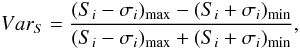 (4)where Smax and Smin are the maximum and minimum value of the flux density at all observation epochs; σSmax and σSmin are their RMS errors. This modification prevents one from overestimating VarS when there are observations with large uncertainties in the dataset. The negative value of VarS corresponds to the case where the estimated error is greater than the observed scatter of the data. The high-frequency variability index versus the spectral index for galaxies (G), quasars (Q), and unidentified radio sources (R) is presented in Fig. 2 which shows all 69 sources that are presented in the Table 3.
One of the main results presented in some earlier papers (Torniainen et al. 2005; Tornikoski et al. 2009, 2001; Aller et al. 2002) is that low variability is, in fact, quite rare among GPS sources identified in the literature. In our sample quasars maintain a relatively constant spectral shape (~20% of total number of quasars in the sample).
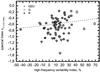 |
Fig. 2 High-frequency variability index vs. the spectral index for galaxies (G), quasars (Q), and unidentified radio sources (R). |
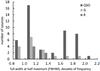 |
Fig. 3 Histogram of the FWHM (in decades of frequency) obtained from a least-squares fit to the radio spectrum of sources with a convex spectrum. |
4.3. Width of the spectra (FWHM)
The width of the continuum spectrum of GPS sources has been studied by O’Dea et al. (1991) and Edwards & Tingay (2004). O’Dea et al. (1991) noted that the narrowest reasonable spectrum, assuming a homogeneous self-absorbed synchrotron source with a power law electron energy distribution, would be 0.77 if the spectral index below the peak is assumed to be +0.8. But observational data demonstrate that the median value in the sample is equal to 1.2. There are only relatively few sources with narrow spectra in our sample (Fig. 3). The FWHM value exceeds a limit of 1.2 for many of them. Figure 3 shows the FWHM distribution of all 69 objects for which this value was determined.
Thus, we also found a lack of sources with narrower spectra. Sources with very narrow FWHM may be selected even if they are hard to find in surveys at discrete radio frequencies (O’Dea et al. 1991). Bright sources such as these with narrow spectra could not be missed in the survey at the frequencies 1.4, 2.7 and 5 GHz, at least most of them. The presence of multiple components with peak at different frequencies will increase the value of FWHM. If some of these components have very narrow spectra, they can remain hidden within the overall spectrum (Snellen et al. 1998).
The relation “redshift–peak frequency–FWHM” for sources with FWHM ≤ 1.3 is shown in Fig. 4. The value limit 1.3 corresponds to sources with inexact convex spectral shape (undetermined spectral shape because of uncertain flux densities or limited frequency range). The peak frequency is presented in the source frame fsource = fobs·(1 + z). As is obvious in Fig. 4, there are two areas with narrower spectra: z ≥ 1.8 (FWHM ≤ 1) and 0.02 ≤ z ≤ 0.7 (the narrowest spectra FWHM ~ 0.9). The first area corresponds to GPS quasars that have statistically higher value of redshift, the second area corresponds to GPS galaxies. But by far the most distant GPS source candidate is the galaxy J1606+31 at z = 4.56 and with a FWHM value 1.1. Additionally, it is necessary to take into account that some GPS source candidates are flat-spectrum radio sources that were included in the sample when they were classified using very sparse data sets.
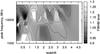 |
Fig. 4 Relation “redshift – peak frequency – FWHM” for sources with FWHM ≤ 1.3. The value limit 1.3 corresponds to the part of sources with inexact convex spectrum shapes because of uncertain flux densities. |
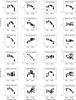 |
Fig. 5 Averaged instantaneous spectra of sources in the sample at several epochs (2006−2010). |
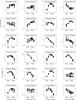 |
Fig. 5 continued. |
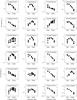 |
Fig. 5 continued. |
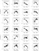 |
Fig. 5 continued. |
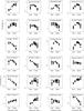 |
Fig. 5 continued. |
5. Discussion
O’Dea (1990) found that approximately half of all ultra-high-z quasars are GPS sources, and likewise half of the GPS quasars are found at ultra-high redshifts. There is a difference in the distribution of redshifts between GPS galaxies and quasars (Snellen 1997; Stanghellini et al. 1998). This may be an indication that a different physical mechanism may play an important role in forming spectral shape in GPS galaxies and quasars.
From VLBI data1, among the detected candidates of GPS galaxies a symmetric structure occurs more often than for GPS quasars. The GPS galaxies statistically demonstrate a symmetric radio morphology (up to hundreds pc) and GPS quasars exhibit a core-jet or complex morphology (from a few pc) (Stanghellini et al. 1997). GPS quasars tend to have the turnover at a higher frequency than galaxies, both in the observed and the rest frame (Snellen 1997; Stanghellini et al. 1998). It has been suggested in Stanghellini (2003) and Snellen et al. (1998) that the GPS quasars and GPS galaxies do not belong to the same population seen from different angles, but that they form two different populations with similar observed shapes of the radio spectra. Variability studies of GPS sources and candidates also indicate that GPS galaxies are less variable than quasar-type GPS sources (e.g. Torniainen et al. 2005; Torniainen et al. 2007). A clear division between high-frequency peaking (HFP) galaxies and quasars was found by Orienti et al. (2006).
The main result of the monitoring is that the mean value of the γ index of the electron energy spectrum (dN(E) = kE−γdE) is 0.5 higher for galaxies (i.e. their energy spectra are steeper) than for quasars. Within the framework of a common model of GPS sources, this fact can be interpreted in the following ways: a) a flatter spectral index for GPS quasars associated with the presence of a flat-spectrum component; b) the observed sample of galaxies (their proper age) is older than the quasar sample (the proper age of quasars); the steepening of their energy spectra is related to additional (in comparison to quasars) age losses of energy for radiation (Kardashev 1962); c) the proper ages of quasar and galaxy samples are approximately identical, but the observed difference in γ is related to the fact that the galaxies in the observed sample were born later than quasars at small z, i.e.there is a cosmological difference in the electron energy spectra.
Of the sample of 122 sources presented in this paper, 56 were found to peak in the cm-domain (see Table 1) and not show very strong variablity (VarS ≤ 25%). These sources seem to adhere to the convex GPS-type spectrum. On the other hand, as can be seen from Fig. 5, many of the remaining 56 GPS-type sources also exhibit some variability at least in some of the observing frequencies, so it cannot completely be ruled out that in some of those cases the convex spectral shapes are still somewhat temporary, caused by flares (disturbances propagating in the jets and with the self-absorption turnover frequency changing with time). It is also worth noting that even though most of the data sets presented in this paper span several years, some of them are as short as approximately two years. As has been shown in variability studies of blazars (Hovatta et al. 2007, 2008), cm-waveband variability time scales can sometimes be considerably long, with strong outbursts occuring once every four to six years and typically lasting for several years. Thus it is highly possible that after an even longer monitoring period some of these sources would also turn out to be variable, blazar-like sources instead of showing GPS-type spectra at all times.
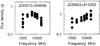 |
Fig. 5 continued. |
Bai & Lee (2005) argued that the GPS quasars (GPSQs) are special blazars – blazars in a dense and dusty gas environment, suggesting that the relativistic jets in GPSQs are oriented at small angle to the line of sight. It is the surrounding dense gas and dust that makes GPSQs show non-blazar properties. On the other hand, some results by Stanghellini (2003) support the view that most of the GPS quasars are like the flat-spectrum radio sources, where a single homogeneous component dominates the radio emission and forms the convex spectrum.
When we constrained our GPS candidate sample even more to include only those sources that have steep, narrow spectra resembling that of a homogenous self-absorbed synchrotron source, we ended up with only 36 sources. Considering the number of sources belonging to the two subtypes in our initial sample, galaxies are over-represented in this final list of GPS sources. This finding also supports the suggestion that compared to quasars, galaxies are more likely to consistently show properties typically associated with GPS-sources over several observing epochs.
6. Conclusions
We have presented the observational results from 12 observing sets (carried out between 2006 and 2010) at the RATAN-600 radio telescope to obtain simultaneous radio spectra, which is valuable and necessary to distinguish genuine GPS sources from flat-spectrum radio sources caught in a flaring state when their spectra are temporarily inverted. The sample contains both quasar- and galaxy-type GPS (122 sources) identified in the literature.
Flux densities at all frequencies were measured at several epochs practically instantaneously – over a period of a few minutes. The observations are result of a long-term programme of “Investigation of radio spectra and variability of GPS sources” (Metsahovi Radio Observatory and SAO RAS). Assuming the generally accepted criteria of radio spectra for homogeneous self-absorbed synchrotron sources, only 17 (14%) objects of our sample were selected as genuine GPS sources. For future work we allowed some slight deviation from the spectral criteria for these sources and chose 19 more GPS candidates. Thus, as a result of monitoring, we have formed a list of 36 (29%) GPS candidates. This agrees well with previous results (Torniainen et al. 2005, 2007; Tornikoski et al. 2009). Obviously the original samples are highly contaminated. This work confirms that the genuine quasar-type GPS sources seem to be very rare.
Some differences were found between the spectral properties of the GPS galaxies and quasars in the sample. The GPS galaxies show a steeper spectral index in the optically thin
part of the spectra (−0.93 ± 0.08 and −0.68 ± 0.05). There are only relatively few sources with narrow spectra in the sample (≤1.2 decades of frequency). The narrowest radio spectra correspond to both ultra-high-z (z ≥ 1.8) and low-z (0.02 ≤ z ≤ 0.7, FWHM ~ 0.9) convex-spectrum radio sources. But the most distant GPS source candidate is the galaxy J1606+31 at z = 4.56 and a value of FWHM = 1.1. The majority of quasars turned out to be variable flat-spectrum radio sources with temporarily inverted spectra and should now be excluded from the GPS candidate lists.
Acknowledgments
The RATAN-600 observations were carried out with the financial support of the Ministry of Education and Science of the Russian Federation (16.518.11.7062 and 16.552.11.7028).
References
- Aller, M. F., Aller, H. D., & Hughes, P. A. 1992, ApJ, 399, 16 [NASA ADS] [CrossRef] [Google Scholar]
- Aller, M. F., Aller, H. D., Hughes, P. A., & Plotkin, R. M. 2002, in Proc. of the 6th EVN Symposium, eds. E. Ros, R. W. Porcas, A. P. Lobanov, & J. A. Zensus, 135 [Google Scholar]
- Bai, J. M., & Lee, M. G. 2005, J. Korean Astron. Soc., 38, 125 [Google Scholar]
- Baum, S. A., O’Dea, C. P., Murphy, D. W., & de Bruyn, A. G. 1990, A&A, 232, 19 [NASA ADS] [Google Scholar]
- Bicknell, G. V., Dopita, M. A., & O’Dea, C. P. 1997, AJ, 485, 112 [Google Scholar]
- Cohen, A. S., Lane, W. M., Cotton, W. D., et al. 2007, AJ, 134, 1245 [NASA ADS] [CrossRef] [Google Scholar]
- de Vries, W. H., Barthel, P. D., & O’Dea, C. P. 1997, A&A, 321, 105 [NASA ADS] [Google Scholar]
- Douglas, J. N., Bash, F. N., Bozyan, F. A., Torrence, G. V., & Wolfe, C. 1996, AJ, 111, 1945 [NASA ADS] [CrossRef] [Google Scholar]
- Edwards, P. G., & Tingay, S. J. 2004, A&A, 424, 91 [NASA ADS] [CrossRef] [EDP Sciences] [Google Scholar]
- Fanti, C., Fanti, R., Dallacasa, D., et al. 1995, A&A, 302, 317 [NASA ADS] [Google Scholar]
- Gopal-Krishna, & Wiita, P. J. 1991, ApJ, 373, 325 [NASA ADS] [CrossRef] [Google Scholar]
- Hovatta, T., Tornikoski, M., Lainela, M., et al. 2007, A&A, 469, 899 [NASA ADS] [CrossRef] [EDP Sciences] [Google Scholar]
- Hovatta, T., Lehto, H. J., & Tornikoski, M. 2008, A&A, 488, 897 [NASA ADS] [CrossRef] [EDP Sciences] [Google Scholar]
- Kardashev, N. S. 1962, Soviet Astron., 6, 317 [Google Scholar]
- Kuehr, H., Witzel, A., Pauliny-Toth, I. I. K., & Nauber, U. 1981, A&AS, 45, 367 [NASA ADS] [Google Scholar]
- Large, M. I., Mills, B. Y., Little, A. G., Crawford, D. F., & Sutton, J. M. 1981, MNRAS, 194, 693 [NASA ADS] [CrossRef] [Google Scholar]
- Massaro, E., Giommi, P., Leto, C., et al. 2009, A&A, 495, 691 [NASA ADS] [CrossRef] [EDP Sciences] [Google Scholar]
- Mingaliev, M. G., Sotnikova, Y. V., Bursov, N. N., Kardashev, N. S., & Larionov, M. G. 2007, AZh, 51, 343 [Google Scholar]
- Mingaliev, M. G., Stolyarov, V. A., Davies, R. D., et al. 2001, A&A, 370, 78 [NASA ADS] [CrossRef] [EDP Sciences] [Google Scholar]
- O’Dea, C. P. 1990, MNRAS, 245, 20 [NASA ADS] [Google Scholar]
- O’Dea, C. P. 1998, PASP, 110, 493 [NASA ADS] [CrossRef] [Google Scholar]
- O’Dea, C. P., Baum, S. A., & Stanghellini, C. 1991, ApJ, 380, 66 [NASA ADS] [CrossRef] [Google Scholar]
- Orienti, M., Dallacasa, D., Tinti, S., & Stanghellini, C. 2006, A&A, 450, 959 [NASA ADS] [CrossRef] [EDP Sciences] [Google Scholar]
- Ott, M., Witzel, A., Quirrenbach, A., et al. 1994, A&A, 284, 331 [NASA ADS] [Google Scholar]
- Pauliny-Toth, I. I. K., Witzel, A., Preuss, E., et al. 1978, AJ, 83, 451 [NASA ADS] [CrossRef] [Google Scholar]
- Pearson, T. J., & Readhead, A. C. S. 1988, ApJ, 328, 114 [NASA ADS] [CrossRef] [Google Scholar]
- Readhead, A. C. S., Taylor, G. B., Xu, W., et al. 1996, ApJ, 460, 612 [NASA ADS] [CrossRef] [Google Scholar]
- Rengelink, R. B., Tang, Y., de Bruyn, A. G., et al. 1997, A&AS, 124, 259 [NASA ADS] [CrossRef] [EDP Sciences] [Google Scholar]
- Rudnick, L., & Jones, T. W. 1982, ApJ, 255, 39 [NASA ADS] [CrossRef] [Google Scholar]
- Shklovskii, I. S. 1960, AZh, 37, 945 [NASA ADS] [Google Scholar]
- Snellen, I. A. G. 1997, Ph.D. Thesis, University of Notre Dame, USA [Google Scholar]
- Snellen, I. A. G., Schilizzi, R. T., de Bruyn, A. G., et al. 1998, A&AS, 131, 435 [NASA ADS] [CrossRef] [EDP Sciences] [Google Scholar]
- Spoelstra, T. A. T., Patnaik, A. R., & Gopal-Krishna. 1985, A&A, 152, 38 [NASA ADS] [Google Scholar]
- Stanghellini, C. 2003, PASA, 20, 118 [NASA ADS] [Google Scholar]
- Stanghellini, C., Baum, S. A., O’Dea, C. P., & Morris, G. B. 1990, A&A, 233, 379 [NASA ADS] [Google Scholar]
- Stanghellini, C., O’Dea, C. P., Baum, S. A., et al. 1997, A&A, 325, 943 [NASA ADS] [Google Scholar]
- Stanghellini, C., O’Dea, C. P., Dallacasa, D., et al. 1998, A&AS, 131, 303 [NASA ADS] [CrossRef] [EDP Sciences] [Google Scholar]
- Tabara, H., & Inoue, M. 1980, A&AS, 39, 379 [Google Scholar]
- Torniainen, I., Tornikoski, M., Lähteenmäki, A., et al. 2007, A&A, 469, 451 [NASA ADS] [CrossRef] [EDP Sciences] [Google Scholar]
- Torniainen, I., Tornikoski, M., Teräsranta, H., Aller, M. F., & Aller, H. D. 2005, A&A, 435, 839 [NASA ADS] [CrossRef] [EDP Sciences] [Google Scholar]
- Tornikoski, M., Jussila, I., Johansson, P., Lainela, M., & Valtaoja, E. 2001, AJ, 121, 1306 [NASA ADS] [CrossRef] [Google Scholar]
- Tornikoski, M., Torniainen, I., Lähteenmäki, A., et al. 2009, Astron. Nachr., 330, 128 [NASA ADS] [CrossRef] [Google Scholar]
- Verkhodanov, O. V. 1997, Astronomical Data Analysis Software and Systems VI, ASP Conf. Ser., 125, 46 [NASA ADS] [Google Scholar]
- Wright, A., & Otrupcek, R. 1990, in PKS Catalog [Google Scholar]
- Zhang, X., Zheng, Y., Chen, H., et al. 1997, A&AS, 121, 59 [NASA ADS] [CrossRef] [EDP Sciences] [Google Scholar]
All Tables
The flux densities of GPS sources and candidates for several epochs (RATAN-600 observations 2006–2010).
Parameters of radio spectra for the sources with spectral maximum (RATAN-600 observations 2006–2010).
All Figures
|
Fig. 1 Flux density calibration factor gν versus focus; where focus is the distance from antenna to the secondary mirror compared to the radius of RATAN-600 (it depends on the antenna elevation) at all wavelengths for the northern sector. All data shown for 9 calibrators were averaged during one observational set in 2007. |
| In the text | |
|
Fig. 2 High-frequency variability index vs. the spectral index for galaxies (G), quasars (Q), and unidentified radio sources (R). |
| In the text | |
|
Fig. 3 Histogram of the FWHM (in decades of frequency) obtained from a least-squares fit to the radio spectrum of sources with a convex spectrum. |
| In the text | |
|
Fig. 4 Relation “redshift – peak frequency – FWHM” for sources with FWHM ≤ 1.3. The value limit 1.3 corresponds to the part of sources with inexact convex spectrum shapes because of uncertain flux densities. |
| In the text | |
|
Fig. 5 Averaged instantaneous spectra of sources in the sample at several epochs (2006−2010). |
| In the text | |
|
Fig. 5 continued. |
| In the text | |
|
Fig. 5 continued. |
| In the text | |
|
Fig. 5 continued. |
| In the text | |
|
Fig. 5 continued. |
| In the text | |
|
Fig. 5 continued. |
| In the text | |
Current usage metrics show cumulative count of Article Views (full-text article views including HTML views, PDF and ePub downloads, according to the available data) and Abstracts Views on Vision4Press platform.
Data correspond to usage on the plateform after 2015. The current usage metrics is available 48-96 hours after online publication and is updated daily on week days.
Initial download of the metrics may take a while.