| Issue |
A&A
Volume 544, August 2012
|
|
|---|---|---|
| Article Number | A108 | |
| Number of page(s) | 6 | |
| Section | Stellar structure and evolution | |
| DOI | https://doi.org/10.1051/0004-6361/201117888 | |
| Published online | 08 August 2012 | |
X-ray follow-up observations of the two γ-ray pulsars PSR J1459–6053 and PSR J1614–2230
1 Université de Toulouse, UPS-OMP, IRAP, 31028 Toulouse, France
e-mail: This email address is being protected from spambots. You need JavaScript enabled to view it.
2 CNRS, IRAP, 9 avenue du Colonel Roche, BP 44346, 31028 Toulouse Cedex 4, France
3 Max-Planck Institute für extraterr. Physik, Giessenbachstrasse 1, 85741 Garching, Germany
4 Max-Planck-Institut für Radioastronomie, Auf dem Hügel 69, 53121 Bonn, Germany
5 Laboratoire de Physique et Chimie de l’Environnement et de l’Espace LPC2E CNRS-Université d’Orléans, 45071 Orléans Cedex 2, France
6 Station de radioastronomie de Nançay, Observatoire de Paris, CNRS/INSU, 18330 Nançay, France
7 Max-Planck-Institut für Radioastronomie, Auf dem Hügel 69, 53121 Bonn, Germany
8 School of Physics and Astronomy, University of Southampton, Highfield, Southampton SO17 1BJ, UK
9 Department of Physics, Royal Institute of Technology, AlbaNova, 10691 Stockholm, Sweden
10 The Oskar Klein Centre for Cosmoparticle Physics, AlbaNova, 10691 Stockholm, Sweden
11 Mullard Space Science Laboratory, University College London, Holmbury St. Mary, Dorking, Surrey, RH5 6NT, UK
12 Institute of Astronomy, University of Zielona Góra, Lubuska 2, 65-265 Zielona Góra, Poland
13 Institut de Ciencies de l’Espai (CSIC-IEEC), Campus UAB, Facultat de Ciencies, Torre C5-parell, 2a planta, 08193 Bellaterra (Barcelona), Spain
Received: 16 August 2011
Accepted: 28 April 2012
Abstract
Aims. We have observed two newly detected γ-ray pulsars, PSR J1459−6053 and PSR J1614−2230, in the X-ray domain with XMM-Newton to try to enlarge the sample of pulsars for which multi-wavelength data exist. We use these data with the aim of understanding the pulsar emission mechanisms of these pulsars.
Methods. We analysed the X-ray spectra to determine whether the emission emanates from the neutron star surface (thermal emission) or from the magnetosphere (non-thermal emission) and compared this to the region in the magnetosphere in which the γ-ray emission is generated. Furthermore, we compared the phase-folded X-ray lightcurves with those in the γ-ray and, where possible, radio domains, to elicit additional information on the emission sites.
Results. J1459−6053 shows X-ray spectra that are best fitted with a power law model with a photon index  . The γ-ray data suggest that either the slot gap or the outer gap model may be best to describe the emission from this pulsar. Analysis of the X-ray lightcurve folded on the γ-ray ephemeris shows modulation at the 3.7σ level in the 1.0−4.5 keV domain. Possible alignment of the main γ-ray and X-ray peaks also supports the interpretation that the emission in the two energy domains emanates from similar regions. The millisecond pulsar J1614−2230 exhibits an X-ray spectrum with a substantial thermal component, where the best-fitting spectral model is either two blackbodies, with
  and 0.88
 keV or a blackbody with similar temperature to the previous cooler component,
  keV and a power law component with a photon index
  . The cooler blackbody component is likely to originate from the hot surface at the polar cap. Analysis of the X-ray lightcurve folded on the radio ephemeris shows modulation at the 4.0σ level in the 0.4−3.0 keV domain.
Key words: X-rays: stars / pulsars: individual: PSR J1459 − 6053 / radiation mechanisms: thermal / stars: neutron / radiation mechanisms: non-thermal / pulsars: individual: PSR J1614 − 2230
© ESO, 2012
1. Introduction
Of the almost 2000 rotationally powered pulsars identified to date (Manchester et al. 2005) the large majority have been detected in the radio domain only. Less than 5% of these pulsars have been detected in the soft X-ray domain (Becker 2009). X-ray pulsations have been detected for only 34 pulsars (Becker 2009; Zavlin 2007; Webb et al. 2004). Just seven pulsars were identified in γ-rays using the high energy instrument EGRET onboard the Compton Gamma Ray Observatory (CGRO), although it was believed that many of the unidentified objects were also associated with pulsars (Helfand 1994). The Fermi Large Area Telescope (LAT) has already identified more than ten times the number of pulsars detected with EGRET (e.g. Abdo et al. 2010a; Ray et al. 2011; Keith et al. 2011) and has even detected many new γ-ray selected pulsars (e.g. Abdo et al. 2009a). The LAT has also detected more than eight Galactic globular clusters in the hard γ-ray domain (>100 MeV, e.g. Abdo et al. 2010b), where the emission is likely to be due to the integrated contribution of millisecond pulsars (MSP), with a total of 2600−4700 MSPs expected in the ensemble of Galactic globular clusters (Abdo et al. 2010b).
X-ray observations and analysis.
One of the many open questions in pulsar physics is the origin of their high-energy emission. Several models have been proposed, which describe the origin of the pulsar high-energy emission. Particle acceleration to extreme relativistic energies could occur in regions of magnetospheric charge depletion (gaps), where very high electric potentials exist. Three main models based on different acceleration region geometries and locations have been proposed: the polar cap (PC), the slot gap (SG) and the outer gap (OG) models (Harding et al. 1978; Arons & Scharlemann 1979; Cheng et al. 1986; Zhang & Harding 2000). Modelling the γ-ray lightcurves in the framework of these models can provide clues as to which model is the most appropriate for a given pulsar (e.g. Venter et al. 2009). Whether one or a combination of these models can account for the high-energy pulsar emission is nonetheless, still an open question.
Additional information can be inferred from X-ray observations. Becker & Trümper (1997), Cheng & Zhang (1998) and others showed that X-ray emission from rotationally powered pulsars can have thermal and non-thermal components. Thermal radiation is expected to arise from the heating of the polar caps by particles returning from the outer magnetosphere, or from the cooling neutron star surface in the case of pulsars (i.e. not millisecond pulsars). Non-thermal emission may be due to the synchrotron emission of charged particles at high altitude. Alternatively, in the framework of the PC model, inverse Compton scattering (ICS) of electron/positron pairs with the soft thermal photons from either the full neutron star surface or the hot polar cap can result in non-thermal X-rays observable in the ~0.1–10.0 keV domain (Zhang & Harding 2000). Bogdanov et al. (2006) also proposed that the non-thermal emission in predominantly thermally emitting MSPs may also be due to Comptonisation of the thermal polar cap emission by energetic electrons/positrons of low optical depth in the pulsar magnetosphere and wind. Inverse Compton scattering and Curvature radiation (CR) pair formation fronts could also play an important role in heating the PC and producing detectable thermal X-rays (Harding & Muslimov 2002). Pulsars that show predominantly thermal X-ray emission can be exploited to constrain the neutron star equation of state (e.g. Bogdanov et al. 2008). By studying the modulation of the observed flux that originates from the evolving projection of the emission from the hot polar cap area through a hydrogen atmosphere, one can infer the ratio of the neutron star mass and the radius (see Bogdanov et al. 2007, and references therein).
Enlarging the sample of high-energy pulsars and comparing their X-ray and γ-ray characteristics is therefore crucial to distinguish between the competing high-energy models and to learn about the neutron star’s composition. The large collecting area and high timing accuracy of XMM-Newton (Jansen et al. 2001) favour reliable spectral and timing studies of pulsars. We present XMM-Newton data of two pulsars that have recently been detected using the Fermi LAT. The first is a γ-ray selected pulsar, J1459−6053 (Abdo et al. 2009a), which has a pulse period of 0.1 s and for which no radio counterpart has yet been identified. A faint X-ray source has been detected with Swift, 9 8 from the γ-ray timing position and tentatively associated with J1459−6053 (Ray et al. 2011). The second is a 3.15 ms pulsar, J1614−2230 (Abdo et al. 2010a). PSR J1614−2230 is particularly interesting because radio observations of this nearly edge-on binary system have revealed a high neutron star mass of 1.97 ± 0.04 M⊙, through the study of the Shapiro delay (Demorest et al. 2010). Chandra and XMM-Newton detections of this pulsar exist, but with insufficient timing resolution to identify X-ray pulsations (Marelli et al. 2011).
2. Data reduction and analysis
Both pulsars have been observed with XMM-Newton, using the three European Photon Imaging Cameras (EPIC Turner et al. 2001; Strüder et al. 2001). For both pulsars the MOS1 and MOS2 cameras were used in imaging mode. The pn camera was used in small-window mode (temporal resolution of 5.7 ms) for J1459−6053. The pn was employed in timing mode for the last of three observations of J1614−2230, with a temporal resolution of ~30 μs, sufficient to resolve any X-ray pulsations of this millisecond pulsar. We considered the last two observations of this pulsar, because they are ~9 and ~5 times longer than the first observation and give the details of these observations in Table 1. We processed the data using the XMM-Newton Science Analysis System (SAS) v11.0.11.
The EPIC observation data files (ODFs) were reduced using the emproc/epproc scripts (for MOS and pn respectively) and the current calibration files (CCFs) dating from 6 July 2011. From the histogram of single events above 10 keV, we identified periods of high background due to soft proton flares. We then selected good time intervals (GTIs) by defining a count rate threshold above the low steady background. We applied standard filtering procedures (e.g. patterns 0−12 for MOS and patterns 0−4 for pn Watson et al. 2009), and kept events between 0.2 and 10 keV for the MOS cameras and between 0.3 and 12 keV for the pn camera. Events contained in energy ranges affected by X-ray fluorescence lines were also filtered2.
Characteristics of J1459−6053 and J1614−2230.
2.1. Spatial analysis
For the X-ray analysis, we first used the source detection task edetect_chain to assess the maximum likelihood of the point sources found in the MOS field of view. The maximum likelihood ML is defined as ML = −ln(pc), with pc the probability for random Poissonian fluctuations to have caused the observed source counts (Watson et al. 2009). We chose a detection threshold MLmin = 10(~4σ), and considered MOS1 and MOS2 datasets simultaneously.
2.2. Spectral analysis
We derived MOS spectra considering the circular extraction regions given in Table 1 and centred on the X-ray source (see Table 2). The regions were chosen to be large enough to include most of the counts from the source, but small enough to exclude close contaminating sources. We extracted pn spectra using the regions corresponding to the observation mode used (imaging or timing) given in Table 1. In each case, we derived corresponding background spectra using a neighbouring area free of X-ray sources and generated instrumental response files. The spectral fitting was performed within Xspec (version 12.5.0)3, using simple models such as a blackbody or a powerlaw (or a combination of these models) describing the thermal and non-thermal emission expected from pulsars, as outlined in Sect. 1. When a blackbody model was employed, the emission radius was calculated using the distance given in Table 2 for J1614–2230 and given in Table 3. The radius determined is highly dependant on the accuracy of the distance used (see e.g. Bogdanov et al. 2007).
2.3. Timing analysis
In the pn timing mode, the events collected from a predefined area are collapsed into a one-dimensional row to be read out at high speed. The pulsar X-ray data are then extracted using a rectangular region centred on the pixel that contains the pulsar. The width of the region, which is the “timing region” given in Table 1, was optimised to obtain the best signal-to-noise ratio (S/N). The background data were similarly extracted by choosing a neighbouring region free of X-ray sources. We used the spectral analysis to indicate the energy interval that yields the best S/N for each pulsar (e.g. Bogdanov & Grindlay 2009). We then used the task barycen to convert times measured in the local satellite frame to Barycentric Dynamical Time (TDB). We used the TEMPO2 package (Hobbs et al. 2006) and the pulsars’ ephemerides to convert the barycentred times of arrival (TOAs) into phase values. For J1614−2230 the ephemeris was provided by the Nançay Radio Telescope, see Table 2 and the ephemeris for J1459−6053, see Table 2, was provided by the Fermi LAT consortium4. The latter ephemeris was calculated directly from the γ-ray data using a maximum-likelihood method for determining pulse times of arrival from unbinned photon data (Ray et al. 2011). We computed the pulse significances using the bin-independent H-test (De Jager & Büsching 2010).
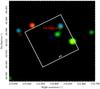 |
Fig. 1 MOS false-colour image of the field around J1459−6053. The field of view is 12′ × 12′. The cross shows the γ-ray timing position of the pulsar (see Table 2). The square shows the size and orientation of the pn small window. The data have been smoothed with a Gaussian. In the online colour version red shows 0.2−0.8 keV photons, green shows 0.8−3.0 keV photons and blue 3.0−10.0 keV photons. |
Based on the barycentred reference profile, we derived phase-aligned pulse profiles using TEMPO2. The derived pulse profiles are based on a reference TOA, thus allowing a reliable phase comparison between the different energy domains.
Simple models fitted to the X-ray spectra of the two pulsars.
3. Results
3.1. J1459–6053
J1459−6053 was detected with a maximum likelihood of ~60 or ~10σ with the MOS cameras at a position RA = 14h59m30 11 ± 067, Dec = −60°53′2129 ± 138 (1σ error values calculated using the statistical error from emldetect and the systematic error from Watson et al. 2009), consistent with the position derived using the ephemeris of the γ-ray counterpart, see Fig. 1 and Table 2, and coincident with the Swift detection of this source (Marelli et al. 2011). The results of the X-ray spectral fitting can be found in Table 3. The X-ray spectrum can be seen in Fig. 2. Using the absorbed power law model, we computed an unabsorbed flux FX = (9.8 ± 1.2) × 10-14 erg cm-2 s-1 (0.2–10.0 keV). Using a reasonable distance assumption of 1 kpc, because no distance has yet been derived for this pulsar, and a beam correction factor, fx of 1 as in, e.g. Marelli et al. (2011), we determine a conversion efficiency, ηX = Lx/Ė, of (8.65
 .
.
Our spectral analysis (see Fig. 2) shows that the X-ray emission is strongest in the 1.0−4.5 keV domain, therefore we chose this energy range for our temporal study. Our X-ray lightcurve contains 378 counts, 198 of which are background counts. Analysis of the lightcurve folded on the γ-ray ephemeris, as described in Sect. 2.3, shows modulation at the 3.7σ level in the 1.0−4.5 keV domain, where the S/N was the highest. This X-ray phasogram can be seen in Fig. 3 along with the γ-ray phasogram taken directly from Ray et al. (2011). For comparison, the 0.3−12.0 keV lightcurve contains 700 counts, with 424 counts associated with the background.
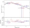 |
Fig. 2 MOS1, MOS2 and pn (black, blue and red crosses, respectively, in the online colour version) X-ray spectrum of J1459−6053 fitted with a power law model (black solid line). |
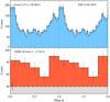 |
Fig. 3 Top: Fermi LAT γ-ray phasogram from Ray et al. (2011), 32 bins per period. Bottom: pn X-ray lightcurve of J1459−6053 (1.0−4.5 keV). The phasogram is shown with 5 bins per period and the dotted line corresponds to the background level. The error bars indicate the statistical 1σ error. Two rotations are shown. Both plots show absolute phase. |
3.2. J1614–2230
J1614−2230 was detected with a maximum likelihood ~100 or ~14σ with the MOS cameras at RA = 16h14m3653 ± 008, Dec = −22°30′3067 ± 126 (1σ error values calculated using the statistical error from emldetect and the systematic error from Watson et al. 2009), consistent with the position of the radio counterpart, see Fig. 4 and Table 2. The results of the X-ray spectral fitting can be found in Table 3. The X-ray spectrum can be seen in Fig. 5. Using the power law plus a blackbody fit, we computed an unabsorbed flux FX = (9.8 ± 0.6) × 10-14 erg cm-2 s-1 (0.2–10.0 keV). Using the distance given in Table 2 and a beam correction factor, fx of 1 as above, we determine a conversion efficiency, ηX = Lx/Ė, of (9.15 .
.
Using the spectral fitting, we determined that the S/N was highest in the 0.4−3.0 keV domain, see Fig. 5. Our X-ray lightcurve in this energy range contains 1543 counts, 1326 of which are background counts. For comparison, the 0.3−12.0 keV lightcurve contains 2842 counts, with 2567 counts associated with the background. Analysis of the lightcurve in the 0.4−3.0 keV domain and folded on the radio ephemeris, as described in Sect. 2.3, shows modulation at the 4.0σ level. This X-ray phasogram can be seen in Fig. 6 along with the γ-ray phasogram taken directly from Abdo et al. (2009b) and the Nançay radio phasogram. The peak observed in the lightcurve, see Fig. 6, is well modelled with a Gaussian centred at φ = 0.66 ± 0.02 and has a full width at half maximum (FWHM) = 0.15 ± 0.07. The peak is aligned, within the errors, with the main γ-ray peak shown in Abdo et al. (2009b), but is shifted by ~0.4 in phase from the main radio peak. However, within 0.05, the X-ray peak is in phase with the secondary radio peak.
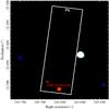 |
Fig. 4 MOS false-colour image of the field around J1614–2230, with the position of the pn camera overplotted. The field of view is 12′ × 12′. The cross shows the radio timing position of the pulsar (see Table 2). The data have been smoothed with a Gaussian. In the online colour version red shows 0.2−0.8 keV photons, green shows 0.8−3.0 keV photons and blue 3.0−10.0 keV photons. |
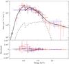 |
Fig. 5 MOS1, MOS2 and pn (black, blue and red crosses, respectively, in the online colour version) X-ray spectrum of J1614−2230 fitted with a blackbody and a power law model (black solid line). |
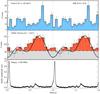 |
Fig. 6 Top panel: Fermi LAT γ-ray phasogram from Abdo et al. (2009b), 20 bins per period. Middle: pn X-ray lightcurve of J1614−2230 (0.4−3.0 keV) overplotted with the model and parameters described in Sect. 4 (black solid line). The phasogram is shown with 16 bins per period and the dotted line corresponds to the background level. The error bars indicate the statistical 1σ error. Bottom: the Nançay 1400 MHz radio lightcurve. All plots show absolute phase. |
4. Discussion
The X-ray spectrum of J1459−6053 appears to be best fitted with a simple power law model, typical of young energetic pulsars, e.g. PSR B1706−44 (Gotthelf et al. 2002). Indeed, the statistically worse blackbody fit indicates an unreasonable small emission radius, see Table 3, for a young pulsar and for a reasonable distance estimate of 1 kpc, supporting the idea that this model does not adequately describe the data. A power law model with a photon index of ~2 can be expected from young pulsars considering any of the three principal models that have been elaborated to describe the high-energy emission of pulsars (see Sect. 1). However, Abdo et al. (2009a) discuss that broad γ-ray beams are required for at least a part of the γ-ray selected pulsar population, because only the high-energy beam but not the relatively narrow radio beam is seen. Such wide, double-peaked light curves are common in outer gap and slot gap models, indicating that this population should have γ-ray emission generated in the outer magnetosphere, near to the light cylinder, which may lend weight to either the SG or the OG model as the most appropriate to describe the emission from this pulsar.
The low value of ηX compared to other similar pulsars, e.g. Marelli et al. (2011), may have been derived because of an underestimated distance or an overestimated beam correction factor. However, Marelli et al. (2011) estimated ηγ with a slightly larger distance of 1.5 kpc and find ηγ > 1. This suggests that the distance estimate must be reasonable and it is just NH that is overestimated. The Fγ/FX = 1081, similar to other radio-quiet pulsars, i.e. Marelli et al. (2011).
A tentative modulation of the folded lightcurve is shown, although because of the low S/N, it is impossible to determine the form/number of any eventual X-ray peak(s). The low S/N in the J1459−6053 lightcurve makes it difficult to compare the X-ray and γ-ray peaks, however, the possible X-ray peak can be seen to be consistent in phase with the γ-ray peak, see Fig. 3 and therefore suggests emission generated in a similar region for the two energy domains.
Fitting the X-ray spectrum of J1614−2230 reveals a good fit for a single-component model. However, a simple power law model reveals a photon index that is unlikely to be physical. It is therefore likely that the MSP is thermally dominated. All thermally dominated MSP, e.g. PSR J0030+0451, PSR J0437−4715 and J2124–3358 (Bogdanov & Grindlay 2009; Bogdanov et al. 2007, 2008) show evidence for a multi-component model. We therefore tried a two-component model, a soft blackbody and either a second harder blackbody or a power law (see Table 3). Marelli et al. (2011) also obtained a similar fit with the same two-component model, although they did not fit the power law component, but used a fixed power law with a photon index of 2. The softer thermal component is expected to come from the heated polar cap(s) of the neutron star (see Sect. 1). Comparing a single-blackbody fit to the two-blackbody fit using the “ftest”, we found a probability of 5 × 10⁻⁵, indicating that the two-component fit is likely at the 4σ level. Owing to the limited S/N of the data presented here, the nature of the harder component is unclear. If it is thermal, it will be caused by non-uniform heating across the polar cap, in a similar way to PSR J0030+0451 (e.g. Becker & Aschenbach 2002; Bogdanov & Grindlay 2009). The two blackbodies correspond to a small, hot region of ~10 m in radius (7−60 m, 90% confidence) and a temperature of ~1.07 × 10⁷ K (0.39−3.9 × 10⁷ K, 90% confidence) and a larger, cooler region of ~530 m radius (320−4960 m, 90% confidence), with a temperature of ~0.17 × 10⁷ K (0.13−0.22 × 10⁷ K, 90% confidence). If it is non-thermal, it may be magnetospheric in origin or arise from inverse Compton scattering of photons closer to the polar cap. The ηX estimated for this MSP is commensurate with other estimates of ηX, e.g. Marelli et al. (2011). The Fγ/FX = 279 and is similar to other radio-loud pulsars i.e. Marelli et al. (2011).
This information can be coupled with the γ-ray and radio data. Venter et al. (2009) modelled the γ-ray and radio data and found that the γ-ray emission is likely to come from the outer gap. The authors proposed a magnetic inclination (α) of ~40° and a viewing angle relative to the rotation axis (ζ) of ~80°. These are approximate values and no formal errors are associated with these estimates. Nonetheless, we can take these estimates at face value and use them in a model like that presented by Bogdanov et al. (2007). The model considers thermal X-ray emission emanating from the polar caps of a neutron star through a non-magnetised light element atmosphere (nsagrav in Xspec Zavlin et al. 1996). This model includes all relativistic corrections necessary for such a compact star. We also include the mass derived by Demorest et al. (2010). This leaves only the radius of the neutron star and the configuration of the dipolar magnetic field as free parameters. Owing to the low S/N of the X-ray lightcurve presented in this paper, detailed modelling is excluded, therefore we use the model in an illustrative manner only. We aim to demonstrate that the observed lightcurve can indeed be described by including the estimates proposed by Venter et al. (2009) and a neutron star with the high mass suggested by Demorest et al. (2010). As can be seen in Fig. 6, the general form of the X-ray lightcurve can be described using these parameters and an offset dipole of the order 10°. For the parameters described above, the offset dipole improves the fit from for example a χ2 = 22.2 (15 degrees of freedom, d.o.f. (no offset dipole)) to χ2 = 10.01 (13 d.o.f., with the offset dipole), when considering a neutron star of radius 11 km. The ftest indicates that the offset dipole is preferred at the 3σ level. This offset is similar to that used by Bogdanov et al. (2007) to model PSR J0437−4715. Including the offset dipole is interesting because it is one of the hypotheses that Venter et al. (2009) used to explain the γ-ray emission observed from MSPs, where the low MSP magnetic field inhibits the creation of sufficient electron-positron pairs, which are ultimately responsible for the γ-ray emission. However, if we remove the constraints imposed on α and ζ from the modelling of the γ-ray lightcurve (Venter et al. 2009), it may be possible to obtain an equally good fit without an offset dipole. More data are required to improve the quality of the lightcurve to allow us to fit an increased number of free parameters to test this hypothesis.
5. Summary
Our X-ray analysis of the young γ-ray selected pulsar J1459−6053 reveals an X-ray spectrum that is best fitted with a power law model, with a photon index, . The γ-ray data suggest that either the SG or the OG model may be best to describe the emission from this pulsar. Analysis of the X-ray lightcurve folded on the γ-ray ephemeris shows modulation at the 3.7σ level in the 1.0−4.5 keV domain. Possible alignment of the main γ-ray and X-ray peaks further supports the interpretation that the emission in the two energy domains emanates from similar regions.
The old millisecond pulsar J1614−2230 shows an X-ray spectrum with a substantial thermal component. It is not clear if the best-fitting spectral model is two blackbodies, with and 0.88 keV or a blackbody with similar temperature to the previous cooler component, keV and a power law component, with a photon index, . The cooler blackbody component is likely to originate from the hot surface at the polar cap. Analysis of the X-ray lightcurve folded on the radio ephemeris shows modulation at the 4.0σ level in the 0.4−3.0 keV domain. This millisecond pulsar shows spectral and temporal similarities with the predominantly thermally emitting millisecond pulsars PSR J0030+0451 and PSR J0437−4715.
Acknowledgments
The X-ray data were made with XMM-Newton, an ESA science mission with instruments and contributions directly funded by ESA Member States and NASA. We thank the anonymous referee for very useful comments that helped to improve this paper.
References
- Abdo, A. A., Ackermann, M., Ajello, M., et al. 2009a, Science, 325, 840 [NASA ADS] [CrossRef] [Google Scholar]
- Abdo, A. A., Ackermann, M., Ajello, M., et al. 2009b, Science, 325, 848 [NASA ADS] [CrossRef] [Google Scholar]
- Abdo, A. A., Ackermann, M., Ajello, M., et al. 2010a, ApJS, 187, 460 [NASA ADS] [CrossRef] [Google Scholar]
- Abdo, A. A., Ackermann, M., Ajello, M., et al. 2010b, A&A, 524, A75 [NASA ADS] [CrossRef] [EDP Sciences] [Google Scholar]
- Arons, J., & Scharlemann, E. T. 1979, ApJ, 231, 854 [NASA ADS] [CrossRef] [Google Scholar]
- Becker, W. 2009, Neutron Stars and Pulsars, Astrophys. Space Sci. Library (Berlin, Heidelberg: Springer), 357 [Google Scholar]
- Becker, W., & Aschenbach, B. 2002, Proc. of the 270. WE-Heraeus Seminar on: Neutron Stars, Pulsars and Supernova Remnants, eds. W. Becker, H. Lesch, & J. Trümper, MPS Report, 278 [Google Scholar]
- Becker, W., & Trümper, J. 1997, A&A, 326, 682 [NASA ADS] [Google Scholar]
- Bogdanov, S., & Grindlay, J. E. 2009, ApJ, 703, 1557 [NASA ADS] [CrossRef] [Google Scholar]
- Bogdanov, S., Grindlay, J. E., & Rybicki, G. B. 2006, ApJ, 648, L55 [NASA ADS] [CrossRef] [Google Scholar]
- Bogdanov, S., Rybicki, G. B., & Grindlay, J. E. 2007, ApJ, 670, 668 [NASA ADS] [CrossRef] [Google Scholar]
- Bogdanov, S., Grindlay, J. E., & Rybicki, G. B. 2008, ApJ, 689, 407 [NASA ADS] [CrossRef] [Google Scholar]
- Cheng, K. S., & Zhang, L. 1998, ApJ, 515, 337 [Google Scholar]
- Cheng, K. S., Ho, C., & Ruderman, M. 1986, ApJ, 300, 500 [NASA ADS] [CrossRef] [Google Scholar]
- De Jager, O. C., & Büsching, I. 2010, A&A, 517, L9 [NASA ADS] [CrossRef] [EDP Sciences] [Google Scholar]
- Demorest, P. B., Pennucci, T., Ransom, S. M., Roberts, M. S. E., & Hessels, J. W. T. 2010, Nature, 467, 1081 [NASA ADS] [CrossRef] [PubMed] [Google Scholar]
- Gotthelf, E. V., Halpern, J. P., & Dodson, R. 2002, ApJ, 567, L125 [NASA ADS] [CrossRef] [Google Scholar]
- Harding, A. K., & Muslimov, A. G. 2002, ApJ, 568, 862 [NASA ADS] [CrossRef] [Google Scholar]
- Harding, A. K., Tademaru, E., & Esposito, L. W. 1978, ApJ, 225, 226 [NASA ADS] [CrossRef] [Google Scholar]
- Helfand, D. J. 1994, MNRAS, 267, 490 [NASA ADS] [Google Scholar]
- Hobbs, G., Edwards, R., & Manchester, R. 2006, Chin. J. Astron. Astrophys. Suppl., 6, 020000 [Google Scholar]
- Jansen, F., Lumb, D., Altieri, B., et al. 2001, A&A, 365, L1 [NASA ADS] [CrossRef] [EDP Sciences] [Google Scholar]
- Keith, M. J., Johnston, S., Ray, P. S., et al. 2011, MNRAS, 414, 1292 [NASA ADS] [CrossRef] [Google Scholar]
- Manchester, R. N., Hobbs, G. B., Teoh, A., & Hobbs, M. 2005, AJ, 129, 1993 [NASA ADS] [CrossRef] [Google Scholar]
- Marelli, M., De Luca, A., & Caraveo, P. A. 2011, ApJ, 733, 82 [NASA ADS] [CrossRef] [Google Scholar]
- Ray, P. S., Kerr, M., Parent, D., et al. 2011, ApJS, 194, 17 [NASA ADS] [CrossRef] [Google Scholar]
- Strüder, L., Briel, U., Dennerl, K., et al. 2001, A&A, 365, L18 [NASA ADS] [CrossRef] [EDP Sciences] [Google Scholar]
- Turner, M. J. L., Abbey, A., Arnaud, M., et al. 2001, A&A, 365, L27 [NASA ADS] [CrossRef] [EDP Sciences] [Google Scholar]
- Venter, C., Harding, A. K., & Guillemot, L. 2009, ApJ, 707, 800 [NASA ADS] [CrossRef] [Google Scholar]
- Watson, M. G., Schröder, A. C., Fyfe, D., et al. 2009, A&A, 493, 339 [NASA ADS] [CrossRef] [EDP Sciences] [Google Scholar]
- Webb, N. A., Olive, J.-F., Barret, D., et al. 2004, A&A, 419, 269 [NASA ADS] [CrossRef] [EDP Sciences] [Google Scholar]
- Zavlin, V. E. 2007, Ap&SS, 308, 297 [NASA ADS] [CrossRef] [Google Scholar]
- Zavlin, V. E., Pavlov, G. G., & Shibanov, Y. A. 1996, A&A, 315, 141 [NASA ADS] [Google Scholar]
- Zhang, B., & Harding, A. K. 2000, ApJ, 532, 1150 [Google Scholar]
All Tables
All Figures
|
Fig. 1 MOS false-colour image of the field around J1459−6053. The field of view is 12′ × 12′. The cross shows the γ-ray timing position of the pulsar (see Table 2). The square shows the size and orientation of the pn small window. The data have been smoothed with a Gaussian. In the online colour version red shows 0.2−0.8 keV photons, green shows 0.8−3.0 keV photons and blue 3.0−10.0 keV photons. |
| In the text | |
|
Fig. 2 MOS1, MOS2 and pn (black, blue and red crosses, respectively, in the online colour version) X-ray spectrum of J1459−6053 fitted with a power law model (black solid line). |
| In the text | |
|
Fig. 3 Top: Fermi LAT γ-ray phasogram from Ray et al. (2011), 32 bins per period. Bottom: pn X-ray lightcurve of J1459−6053 (1.0−4.5 keV). The phasogram is shown with 5 bins per period and the dotted line corresponds to the background level. The error bars indicate the statistical 1σ error. Two rotations are shown. Both plots show absolute phase. |
| In the text | |
|
Fig. 4 MOS false-colour image of the field around J1614–2230, with the position of the pn camera overplotted. The field of view is 12′ × 12′. The cross shows the radio timing position of the pulsar (see Table 2). The data have been smoothed with a Gaussian. In the online colour version red shows 0.2−0.8 keV photons, green shows 0.8−3.0 keV photons and blue 3.0−10.0 keV photons. |
| In the text | |
|
Fig. 5 MOS1, MOS2 and pn (black, blue and red crosses, respectively, in the online colour version) X-ray spectrum of J1614−2230 fitted with a blackbody and a power law model (black solid line). |
| In the text | |
|
Fig. 6 Top panel: Fermi LAT γ-ray phasogram from Abdo et al. (2009b), 20 bins per period. Middle: pn X-ray lightcurve of J1614−2230 (0.4−3.0 keV) overplotted with the model and parameters described in Sect. 4 (black solid line). The phasogram is shown with 16 bins per period and the dotted line corresponds to the background level. The error bars indicate the statistical 1σ error. Bottom: the Nançay 1400 MHz radio lightcurve. All plots show absolute phase. |
| In the text | |
Current usage metrics show cumulative count of Article Views (full-text article views including HTML views, PDF and ePub downloads, according to the available data) and Abstracts Views on Vision4Press platform.
Data correspond to usage on the plateform after 2015. The current usage metrics is available 48-96 hours after online publication and is updated daily on week days.
Initial download of the metrics may take a while.