| Issue |
A&A
Volume 543, July 2012
|
|
|---|---|---|
| Article Number | A158 | |
| Number of page(s) | 9 | |
| Section | The Sun | |
| DOI | https://doi.org/10.1051/0004-6361/201219164 | |
| Published online | 17 July 2012 | |
Spectropolarimetric signatures of anisotropic velocity distributions of optically thin coronal UV lines
1 Dipartimento di Fisica e Astronomia, SASS, Università degli Studi di Firenze, Largo E. Fermi 2, 50125 Firenze, Italy
e-mail: This email address is being protected from spambots. You need JavaScript enabled to view it.
2 INAF – Osservatorio Astronomico di Torino, Strada Osservatorio 20, Pino Torinese (TO), Italy
Received: 5 March 2012
Accepted: 6 June 2012
Abstract
Context. Many interpretations of observations with the Ultraviolet Coronagraph Spectrometer (UVCS) operating aboard the Solar and Heliospheric Observatory (SOHO) have suggested that there are variations in particle velocity distributions. In this paper, we investigate their spectropolarimetric signatures.
Aims. We uncover the spectropolarimetric signatures of anisotropic velocity distribution functions after a line-of-sight (LOS) integration of both the 1215.16 Å Lα line and the 1032 Å O vi line.
Methods. We perform a forward modelling of the resonance scattering of neutral hydrogen atoms and O5+ ions in the presence of anisotropic velocity distribution functions using a self-consistent 2.5-dimensional, magnetohydrodynamics global coronal model. We analyse the most important observables in spectropolarimetry, i.e., the rotation of the plane of linear polarisation, and de-or hyperpolarisation after a LOS integration.
Results. The spectropolarimetric signatures of anisotropic velocity distributions do survive the LOS integration, and are to be found in the region where there are non-radial solar outflows, i.e., from mid-way between the poles and the equator and down to the equator, in some cases starting from the photosphere all the way out to almost 2 R⊙. We consider the cases of w⊥ = 2w and w∥ = w or w ⊥ = w and w∥ = 2w, where w is the local thermal velocity of either neutral hydrogen atoms or O5+ ions, and where w⊥ and w∥ characterise the perpendicular and parallel distributions of the components of the velocity with respect to the magnetic field, respectively. We find that the rotation angles reach values of roughly ± 15 degrees, and should in principle be measurable.
Conclusions. Our results show that it should be possible to distinguish anisotropic velocity distribution functions on the condition that one samples as extensive a region of the plane of the sky as possible. The effects of the anisotropy are in most cases seen all the way out to 2 R⊙, and we therefore recommend that the observations be made as far away from the photosphere as possible in order to avoid the possible contamination by active regions. It will in most cases, however, be extremely hard to determine the sense of the anisotropy using only spectropolarimetry.
Key words: Sun: corona / Sun: UV radiation / polarization / radiative transfer
© ESO, 2012
1. Introduction
Spectropolarimetry is one of the most valuable remote-sensing techniques presently available. It holds the promise of unveiling many of the most important elusive solar atmospheric plasma parameters, such as the magnetic field vector, the solar-wind velocity vector, and the particle microscopic velocity distribution functions. Detailed empirical knowledge of the physical state of the coronal plasma is a sine qua non for understanding the basic physics underlying the extremely varied solar phenomenology.
This paper is the third in a series devoted to the investigation of the diagnostic content of optically thin resonantly scattered coronal ultraviolet (UV) lines after a line-of-sight (LOS) integration. In the first paper, Khan et al. (2011, Paper I), we investigated the consequences of the presence of three polarimetrically active agents on the linear polarisation parameters for the first three lines of the Lyman-series, i.e., magnetic fields, non-radial outflow velocities, and the presence of active regions on the solar surface, using a self-consistent 2.5-dimensional, magnetohydrodynamics (MHD) global coronal model with a solar minimum-like magnetic field topology, i.e. a global dipole field directed along the Sun’s polar regions with a current-sheet-like structure in the equatorial plane, and strengths that lie in the realistic range of a few gauss. In the second paper, Khan & Landi Degl’Innocenti (2011, Paper II), we focused on the symmetry aspects inherent in the linear polarisation parameters owing to active regions emitting in the Lα line, using a spherically symmetric coronal model.
One of the primary objectives of the Ultraviolet Coronagraph Spectrometer (UVCS) operating aboard the Solar and Heliospheric Observatory (SOHO, Kohl et al. 1995, 1997), was to obtain accurate measurements of the outflow velocities and the microscopic velocity distribution functions in the principal acceleration regions between roughly 1 and 4 R⊙ in the low-density polar open-field regions during solar minimum conditions and beyond.
Most of the initial interpretations of UVCS data have concluded that there must be both intense preferential heating of O5+ ions compared to protons, and a strong anisotropy in the microscopic velocity distribution functions with respect to the magnetic field direction, with the most probable perpendicular speed being possibly up to two orders of magnitude greater than the parallel one (Kohl et al. 1997; Li et al. 1998; Cranmer et al. 1999; Antonucci et al. 2000). Not everybody, however, agrees with this interpretation. In Raouafi & Solanki (2004, 2006), the authors make different assumptions especially about the radial variation in the electron density, and conclude that the need for a strong anisotropy in the velocity distribution functions may not be as compelling as most of the initial papers suggested. This in turn prompted Cranmer et al. (2005), Kohl et al. (2006), and Cranmer et al. (2008) to re-examine an extended collection of UVCS data to determine the O5+ properties more reliably, but their conclusions remain the same, i.e., that there appears to be both a preferential heating of O5+ ions compared to protons and highly anisotropic velocity distribution functions.
Intrigued by these non-intuitive plasma properties, we set ourselves the goal of performing a parameter study of the spectropolarimetric consequences of anisotropic velocity distributions of neutral hydrogen atoms and O5+ ions using the same coronal MHD model as Paper I.
The nature of our study is exploratory, and all the cited papers have had an inspirational influence on this paper. Our goal is not to reproduce any of the conditions considered in these papers in order to check whether spectropolarimetry could be used as an “independent judge” when it comes to deciding e.g. whether the UVCS data is best interpreted with or without anisotropic velocity distribution functions. Most of our graphs do not go much beyond 2 R⊙, mainly because of the weaker signals at higher altitudes, and it is generally agreed that velocity distribution functions are isotropic within 2 R⊙.
It is, however, instructive to analyse whether even slight anisotropies in the velocity distribution functions in optically thin coronal UV lines survive LOS integrations, and, if yes, what their spectropolarimetric signatures are, i.e., rotation of the plane of linear polarisation, and de-or hyperpolarisation of the scattered radiation, where to locate them in global graphs, and, last but not least, to relate the findings to the effects of previously studied polarimetrically active agents.
In Sect. 2, we present the coronal and atomic models, and in Sect. 3 we briefly present the equations for resonance polarisation in the presence of collisions and anisotropic velocity distribution functions. Section 4 is dedicated to presenting and discussing our simulation results. Finally, in Sect. 5 we sum up all the conclusions.
2. The coronal model and atomic parameters
The solar coronal MHD model used in this paper is given in Wang et al. (1993). It is a self-consistent 2.5-D, MHD global coronal model with a solar minimum-like magnetic field topology, i.e. a global dipole field directed along the Sun’s polar regions with a current-sheet-like structure in the equatorial plane, and strengths that lie in the realistic range of a few gauss. In Figs. 1a, b, we display the electron density and the temperature profile at mid-latitude, i.e., at 45 degrees, respectively, and in Figs. 1c, d we show the magnetic and velocity structures in the plane of the sky. All the atomic parameters for the 1215.16 Å Lα line can be found in Paper I. The 1032 Å O vi line corresponds like the Lα line to an atomic transition with Ju = 3/2 and Jℓ = 1/2, where J is the total angular momentum, and ranks after the Lα line as one of the strongest spectral lines emitted by the solar corona (Vial et al. 1980; Raymond et al. 1997). In contrast to the Lα line, it is formed by both electron collisions and the resonance scattering of the partially anisotropic radiation from the solar disk.
 |
Fig. 1 The solar coronal MHD model. |
The collisional excitation depends on the collision rate, αc, which is a function of the electron temperature and fitted in Cranmer et al. (2008) as  (1)where t = log 10(Te), and αc and Te are given in units of cm3 s-1 and K, respectively. The velocity distribution function of the electrons is assumed to be a simple Gaussian function.
The radiative excitations depend sensitively on the intensity profiles incident from the solar disk, and we have adopted Gaussian profiles derived empirically with total intensities measured by UVCS on the disk at solar minimum and given by 524 × 1013 and 1.94 × 10¹³ photons s-1 cm-2 sr-1 (Raymond et al. 1997). We do not consider any centre-to-limb variation in the intensity emitted by the solar disk for any of the lines. The profile widths are taken from Cranmer et al. (1999) and Noci et al. (1987), respectively. For the logarithm of the ratio of hydrogen atoms to protons, we refer to Fig. 1d of Paper II. The ion concentration ratio of nO5 + /np is fixed at 1.5 × 10⁻⁶ (Cranmer et al. 2008), and we assumed a helium to hydrogen number density ratio of 5%.
3. Theory
In Paper I, we presented the most important formulae for resonance scattering of neutral hydrogen atoms in the presence of the pumping anisotropic radiation field coming from the solar chromosphere, magnetic fields, non-radial outflows, and active regions. In this section, we add the formula for two additional important contributions capable of altering the polarisation signatures of the O vi line, namely collisions and anisotropic velocity distribution functions. For additional details about the theory of resonance scattering of polarised radiation, we recommend that the interested reader consult the monograph “Polarisation in Spectral Lines” by Landi Degl’Innocenti & Landolfi (2004), hereafter LL04.
Our coordinate system (x,y,z) has its origin at the centre of the Sun. The y axis is directed in the observer-Sun direction, while the z axis lies in the plane of the sky, and is directed such that the (y,z) plane contains the Sun’s rotation axis and points towards the solar north pole. The x axis is also in the plane of the sky and directed in a manner that (x,y,z) forms a right-handed coordinate system. The coordinates are expressed in units of solar radii, R⊙ = 6.9626 × 10⁵ km. The “observations” are made around the Sun in an equidistant rectangular grid ranging from ±2 R⊙ in the plane of the sky and ±~7 R⊙ along the LOS. Through trial and error, we found that there were no changes up to the fourth significant figure in the four Stokes emission coefficients if the step size of the numerical integration was 0.03 R⊙ along the LOS. For a given LOS, i.e., (x,z), the code calculates the four emission coefficients for all the points along it, thus giving rise to all sorts of different scattering geometries with varying magnetic and velocity fields as given by the coronal model.
3.1. Resonance polarisation in the presence of collisions and anisotropic velocity distribution functions
The oxygen ions are described in terms of the multipole moments of the density matrix in the spherical statistical tensor representation, and are modelled to have only two levels, an upper level with Ju = 3/2, and a lower one with Jℓ = 1/2. Assuming the lower level to be unpolarised and neglecting stimulation effects owing to the dilution of the solar radiation in the FUV, one arrives, after solving the statistical equilibrium equations, at the expression for the upper level multipole moments of1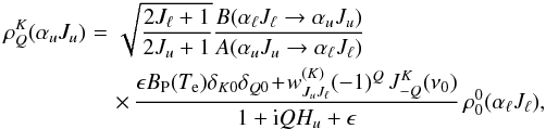 (2)where
  , and
, and  is the superelastic collisional rate2 and represents the ratio of collisional to radiative de-excitation rates of the upper level, while
 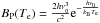 is the Planck function in the Wien limit. All the other quantities have their usual meaning.
The radiation field tensor is given by 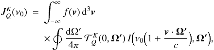 (3)where the velocity distribution function is given by
 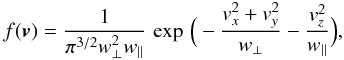 (4)which is a so-called bi-Maxwellian, that, in contrast to the usual Maxwellian distribution has two parameters, w⊥ and w∥, characterising the perpendicular and parallel distributions of the components of the velocity with respect to the magnetic field, respectively.
The frequency-integrated emission coefficients along a given direction Ω are given by
![Mathematical equation: \begin{eqnarray} \tilde{\epsilon_i}(\vec{\Omega})& =& k^{\rm A}_{\rm L}\Bigg[\frac{\epsilon}{1+\epsilon}B_{\rm P}(T_{\rm e})\delta_{i0}\nonumber \\ &&\quad + \!\sum_{KQ}\! W_K(J_{\ell},J_u) \, (-1)^Q \, \mathcal{T}^K_{Q}(i,\vec{\Omega}) \, \frac{1}{1\!+\!{\rm i}QH_u\!+\!\epsilon} \, J^K_{-Q}(\nu_0)\Bigg], \label{eq4} \end{eqnarray}](/articles/aa/full_html/2012/07/aa19164-12/aa19164-12-eq46.png) (5)where
(5)where  is the frequency-integrated absorption coefficient of the line. The emergent Stokes parameters are finally obtained by integrating the emissivity along the LOS.
The inclusion of collisions in our description of resonance scattering has two effects. On the one hand, they introduce an additional term that only affects the intensity and not the polarisation characteristics of the scattered radiation3, and is proportional to  , which can be written as
  , and represents the collisional de-excitation rate divided by the total de-excitation rate of the upper level. On the other hand, one can write
  , with
  , where the dimensionless parameter Hu is given by
  .
.
In resonance scattering with collisions,  , which can potentially diminish the impact of the magnetic field as a de-or hyperpolarising agent in the Hanle effect.
4. Results
This section is divided into four subsections. In the first, we present numerical examples of some of the vital parameters in resonance scattering with collisions. It deals exclusively with the O vi line. All equivalent information on the Lα line can be found in Paper I. In the second and third subsections, we show simulations where we have parametrised w⊥ and w∥ for the Lα and O vi lines, respectively.
4.1. The contributions to the intensity, the degree of linear polarisation, and the number of photons
In all the graphs in this subsection, the quantities depicted are functions of the distance from the solar surface in the plane of the sky at mid-latitude, i.e., the symmetry line that bisects the first quadrant with polar angle equal to π/4. The reason for choosing this particular polar angle is, as we show, that one needs non-radial outflows in order to see the spectropolarimetic signatures of anisotropic velocity distribution functions. These are to be found predominantly in the interface region where the magnetic field lines go from being open to closed, i.e., at a polar angle of π/4.
The first graph shows ϵ, i.e., the ratio of the collisional to the radiative de-excitation rates of the upper level. It starts out at 10-8.5 and then decreases roughly linearly with the electron density. From its smallness, we can deduce two results, i.e., on the one hand that radiative de-excitation rates completely overpower collisional de-excitation rates, and on the other hand that the efficiency of the magnetic field as a de-or hyperpolarising agent in the Hanle effect is unaltered. Hu and  as defined in the previous section are, for all practical purposes, the same.
The second graph shows the radiative and collisional contributions to the emitted intensity. The collisional component starts out at 10-7.9 erg cm-3 s-1, and then falls off as a quadratic function of the electron density. The radiative component starts out at 10-9.7 erg cm-3 s-1, and then falls off linearly with the electron density. The reason why the decrease is more pronounced than in the collisional case is that as the solar wind picks up speed the scattering ions progressively fall out of resonance, and see less and less of the incoming radiation at the transition frequency, i.e., it is Doppler-dimmed.
The third graph shows the fractional linear polarisation defined as  × 100%, where I = (I,Q,U,V)T is the usual Stokes vector, after a LOS integration. This quantity constitutes together with the rotation of the plane of linear polarisation the most important observable in polarimetry. It is an increasing function with a maximum of about 0.7% at 1.6 R⊙, and then gradually decreases. These values differ radically from those provided by Raouafi et al. (2002a) by an order of magnitude. The reason for this discrepancy is that we employ the electron density given by the coronal model of Wang et al. (1993), whereas Raouafi et al. (2002a) assume a value that happens to be smaller by more than an order of magnitude. For a discussion and a table of representative values of electronic densities employed by various models and their practical consequences for the resonance polarisation of the O vi line (we refer to Khan 2012). PL is very sensitively dependent on the electronic density, and it remains an open problem whether the value measured by Raouafi et al. (2002a) is too high and the modelled electronic density too low, or whether the electronic density employed by Wang et al. (1993) is too high and the ensuing fractional linear polarisation reported in this paper too low. This issue will probably only be resolved by new measurements of both quantities made simultaneously. The condition for the O5 + ions to harbour polarisation (hence be aligned) and thus capable of emitting polarised radiation is the existence of an anisotropic radiation source, in this case the Sun. The further away the scattering ion is from the Sun, the more anisotropically it perceives the radiation and the more linearly polarised radiation it emits. The reason why this increase in linearly polarised scattered radiation is halted and inverted is two-fold. On the one hand, the radiatively scattered component slips progressively out of resonance as the solar wind increases, and on the other hand the intensity of the collisional component falls off less steeply and thus decreases the degree of linear polarisation yet more.
The fourth graph shows the number of photons per unit area per unit time per unit solid angle after a LOS integration. It starts out at roughly 1014 cm-2 s-1 sr-1 at the solar surface and then diminishes to roughly 1012 cm-2 s-1 sr-1 at 1.6 R⊙, meaning that the number of polarised photons available for detection at the distance where the degree of linear polarisation was a maximum is approximately 7 × 109 cm-2 s-1 sr-1. These values must be stringently observed by instrumentalists because they severely constrain the necessary measurement sensitivity needed in order to use spectropolarimetry as a tool for inferring plasma parameters.
For comparison, we briefly cite the corresponding values for the Lα line. The degree of linear polarisation increases monotonically and reaches values of up to ~15.3% at 1.6 R⊙, and the number of photons per unit area per unit time per unit solid angle after a LOS integration varies from roughly 1013 cm-2 s-1 sr-1 at the solar surface and then diminishes to roughly 1011 cm-2 s-1 sr-1 at 1.6 R⊙, giving approximately 5 × 1010 cm-2 s-1 sr-1 polarised photons at this distance.
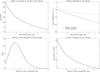 |
Fig. 2 An exploration of some of the vital parameters of spectropolarimetry of the O vi line. |
4.2. Spectropolarimetric signatures of anisotropic velocity distributions for the Lα line
Spetropolarimetric signatures are most accurately analysed using two quantities, namely the rotation angle, Dα, defined as the difference, measured counterclockwise in degrees, of the polarisation angle, α, given by tan(2α) = U/Q, with respect to the parallel to the solar limb4, and the de-or hyperpolarisation defined as PL − P0. Usually P0 is defined as the degree of linear polarisation in the absence of symmetry-breaking effects (magnetic fields, non-radial outflows, etc.), but here we define it as the degree of linear polarisation in the presence of magnetic fields and non-radial outflows in order to show what changes are to be expected based solely on the introduction of anisotropic velocity distribution functions.
In Sahal-Bréchot et al. (1998), the authors thoroughly discuss the spectropolarimetric consequences of non-radial solar outflows, which we were able to confirm with our simulations in Paper I, even after a LOS integration5. Inspired by the possibility of anisotropic velocity distribution functions proposed by most interpretations of the UVCS/SOHO data, Fineschi (2001) analysed the consequences of the addition of anisotropic velocity distribution functions onto non-radial solar outflows, and showed that this considerably alters the polarisation parameters.
Intrigued by these findings and in order to remain faithful to our mission of uncovering the signatures of as many polarimetrically active agents as possible, we parametrised both w⊥ and w∥ to examine their effects after a LOS integration.
We parametrised w⊥ and w∥ as functions of the local thermal velocity of the neutral hydrogen atoms, given by  , i.e., w⊥ = c⊥w and w∥ = c∥w. Ideally, and especially if one had observational data with which to compare one’s simulations, one would have to search all of the relevant parameter space, that is, find appropriate step-sizes for c⊥ and c∥, respectively, and compare the resulting points in two-dimensional parameter space to the observations. Unfortunately, however, we did not have any observational data with which to compare our forward-modelling results, and did not therefore perform a full search of parameter space. Our approach was more qualitative in that we tried to understand the general characteristics of introducing anisotropies in the velocity distribution functions, focusing on how and where they modify the polarimetric landscape.
In Figs. 3a − c, we have shown Dα for the isotropic case (upper left graph), the anisotropic cases with w∥ = 2w, and w⊥ = w (upper right graph), and w∥ = w, and w ⊥ = 2w (lower left graph), respectively. Figure 3d shows the de-or hyperpolarisation for the anisotropic case with w∥ = 2w, and w⊥ = w.
 |
Fig. 3 Dα for the isotropic case (upper left graph), the anisotropic cases with w⊥ = 2w, and w∥ = w (upper right graph), and w∥ = 2w, and w⊥ = w (lower left graph), respectively. The lower right graph is the de-or hyperpolarisation for the anisotropic case with w⊥ = 2w, and w∥ = w. All graphs are for the Lα line. |
Figure 3a is the isotropic case and one can easily discriminate between the rotations due to the magnetic field above the poles, and those due to the non-radial outflows midway between the poles and the equator. The angles are roughly one tenth of a degree for both agents. In Fig. 3b, we have doubled the most probable perpendicular speed w⊥ = 2w with respect to the local thermal velocity and the changes are staggering. The clearly defined “arms” have radically changed shape. The most pronounced effects are now seen very close to the solar surface almost all the way from the poles to the equator, and some of the “arm” structure becomes less prominent towards the equator, persisting out to roughly 1.8 R⊙. The signatures of the magnetic field over the poles have been completely eclipsed and are now dominated entirely by the effects of the anisotropic velocity distribution functions. Interestingly, the angles have increased by two orders of magnitude, which bodes well for spectropolarimetric observations since such relatively great angles should be easily detectable. In Fig. 3c, we have inverted the sense of the anisotropy, i.e., assume that w∥ = 2w and w⊥ = w. This has the non-intuitive effect of creating a left-right symmetry in that the right-and left-hand side of Fig. 3b is roughly equal to the left- and right-hand side of Fig. 3c. Finally, in Fig. 3d we show the de-or hyperpolarisation for the anisotropic w∥ = 2w, and w⊥ = w case. The maximum and minimum values are roughly 0.41% and −1.47%, indicating that anisotropic velocity distribution functions both de-and hyperpolarise, and their appearance is closely correlated to the maximum and minimum rotations in the corresponding Dα graphs.
The de-and hyperpolarisations found are very small compared to the rotations, and, based on the degree of linear polarisation of one or a few LOS’, we are unable to tell whether anisotropic velocity distribution functions are at play. It clearly emerges from Fig. 3d that the signature lies in the pattern displayed and that one needs as large a portion of the sky as possible in order to detect and decipher it.
What happens if one explores parameter space for values of c ⊥ and c∥ in-between 1 and 2, or even beyond? How does one go for instance from the positive rotations in the regions of the upper right arms of Fig. 3a to the negative rotations in the same region of Fig. 3b? Our simulations show that the onset of morphological change occurs for anisotropies as small as c∥ or c ⊥ equal to ≈1.005. The rotations and de-or hyperpolarisations are still small, but increase steadily with increasing anisotropy. There are many interesting morphological changes for c∥ or c⊥ up to ≈1.1, after which it saturates, i.e., the graphs all look alike. The rotation angle, however, keeps on increasing as the parameters increase as is shown in Table 1. This is a very interesting finding because it suggests that if one achieves the necessary measurement sensitivity, spectropolarimetry could in principle reveal the onset of anisotropy, which, needless to say, would be very important for furthering the understanding of the local microscopic processes that are involved in accelerating the solar wind.
The graphs presented in Figs. 3 are global. This means that one only sees the most predominant contributions. The overpowering effect of some regions eclipses the effects of other regions that, if analysed separately, could possibly yield measurable rotations and de-or hyperpolarisations. This means that one must be very careful when analysing these graphs in order to use them for finding the most appropriate portions of the plane of the sky on which to perform spectropolarimetry. Depending on the characteristics of the instrument, one has to subdivide the plane of the sky into smaller portions and make local graphs to assess the feasibility of performing spectropolarimetry on them.
The rotation angle for various values of the anisotropy parameter c⊥, with c∥ = 1.
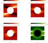 |
Fig. 4 Dα for the isotropic case (upper left graph), the anisotropic cases with w⊥ = 2w, and w∥ = w (upper right graph), and w∥ = 2w, and w⊥ = w (lower left graph), respectively. The lower right graph is the de-or hyperpolarisation for the anisotropic case with w⊥ = 2w, and w∥ = w. All graphs are for the O vi line. |
The signatures displayed are obtained after a LOS integration and it is therefore not a simple task to provide an exhaustive explanation of the outcome. One can, however, say the following. For any point along the arm on the upper right-hand side of the solar atmosphere in Fig. 3a, the rotation of the plane of linear polarisation is positive. It is so because as the direction of the radiation, Ω, becomes more perpendicular to the velocity, the less-Doppler shifted it is. Comparing with Fig. 1d, this means that the radiation coming predominantly from below will be less Doppler-shifted and thus felt more intensely by the scattering atom, and will as a consequence rotate the plane of linear polarisation towards aligning itself with that direction. This is the basic physics that one has to keep in mind when analysing the rotation for each point along the LOS, be that with or without anisotropic velocity distributions. In the latter case, the analysis is obviously much more complicated. The important lesson to learn from the simulations is that non-radial outflows with or without anisotropic velocity distribution functions do have measurable spectropolarimetric consequences.
Is any solution of parameter space unique? Can one tell the sense of the anisotropy, i.e., which of w⊥, w∥ is greater unequivocally? The answer to this question depends heavily on the size of the portion of the plane of the sky that we have data from. The more extensive the region is, the higher the probability of discerning the sense of the anisotropy. On the basis of excursions into parameter space, the sober preliminary answer is probably that one will be unable to distinguish the sense of the anisotropy solely by spectropolarimetry, but this remains unclear.
What other polarimetrically active agents are operative in the area where the signatures of anisotropic velocity distribution functions can be seen? Active regions in the photosphere are capable of modifying the linear polarisation parameters through two effects that occur simultaneously, namely intensity contrasts, ΔIν, that break the locally cylindrical symmetric radiation field brought about by the relatively intense magnetic fields, and the magnetic fields themselves. The breaking of the locally cylindrical symmetric radiation field was discussed thoroughly in Sect. 3 of Sahal-Bréchot et al. (1986), where it is made clear that any attempts to diagnose coronal plasma parameters must be accompanied by spectroheliograms that reveal the presence of active regions that modify the linear polarisation parameters in their immediate vicinity. Modifications may also be caused by the global background field. Our simulation results show that the effects of anisotropic velocity distribution functions should persist substantially beyond the regions that would be affected by active regions, and our recommendation is therefore to do the observations as far away from the photosphere as possible. The presence of magnetic fields can, however, be detected by analysing the region with other lines that have a different sensitivity to the magnetic field, or by classical longitudinal Zeeman spectropolarimetry combined with linear polarisation measurements in forbidden emission lines, as suggested in Judge et al. (2006) and Peter et al. (2012).
Ultimately, the successfulness of this method will depend on how extensive a portion of the plane of the sky one can sample. The smaller the region is, the less likely it will be that we can interpret the measurements correctly.
4.3. Anisotropic velocity distributions of the O VI line
We now repeat the exercise described in the previous subsection for the O vi line. The thermal velocity of the O5 + ions is in this case roughly four times smaller than that of the hydrogen atoms, and is given by  . The isotropic case is morphologically identical to the Lα one, but the rotation angles are one order of magnitude greater, i.e., ±1.35°. This means that the rotations of roughly ±0.15° caused by the magnetic field above the poles are harder to discern.
In Figs. 4b and c, we again double the most probable perpendicular and parallel speeds, respectively, and obtain more or less the same results as we did for the Lα case. The non-intuitive left-right symmetry of Figs. 3b, c is not exactly maintained for this line, and it probably occurs for slightly different values of the parameters. The de-or hyperpolarisation graph for w⊥ = 2w, and w∥ = w shows values ranging from roughly −0.17% to 0.28%, again indicating that anisotropic velocity distribution functions both de-and hyperpolarise. As for the Lα line, the values are very small, the signature lies in the pattern displayed, and one will need as large a portion of the sky as possible in order to detect and decipher it.
Given the overpowering brightness of the Lα line relative to the O vi line, and the much higher degree of linear polarisation due almost to exclusively radiative excitation, and the similarity between the rotations and de-or hyperpolarisations, the Lα line is clearly a more suitable diagnostic than the O vi line.
5. Conclusions
The spectropolarimetric analysis of optically thin UV lines in order to determine vital plasma parameters could prove to be a very promising development in the future. Much theoretical modelling, however, needs to be undertaken.
The preliminary synthesis of LOS-integrated Stokes emission coefficients incorporating as many polarimetrically active agents as possible is pivotal to understanding the true potential of this remote-sensing technique. To what extent do the effects of magnetic fields, non-radial outflows etc. survive LOS integrations, what are their signatures, and how does one disentangle the possible simultaneity of active agents? The goal of papers similar to the present one is to answer these questions by showing the simulation results of the realistic forward modelling of solar coronal physics.
In this paper, we have looked at the spectropolarimetric consequences of anisotropic velocity distribution functions using a self-consistent coronal model with non-radial solar outflows for the 1215.16 Å Lα and the 1032 Å O vi lines. For each of these lines, we have commented on whether the effects survived a LOS integration, and if yes, where to find them, and by how much they rotated the plane of linear polarisation, and whether they had a de-or hyperpolarising effect. Last but not least, we have also tried to relate these findings to previously known active agents.
For the Lα line, the results show that even slight anisotropies survive the LOS integration, and that the global signatures differ radically from the isotropic ones. They are located mid-way between the poles and the equator and extend down to the equator, in the regions of non-radial solar outflows, and, in certain cases, extend all the way out to almost 2 R⊙. Other polarimetrically active agents in the region are active regions on the solar surface, and much care must be taken to disentangle the various contributions correctly. Our recommendation is to do observations as far out as possible, and in as extensive a region of the plane of the sky as possible. Large rotation angles and their sense of rotation will prove to be the spectropolarimetric signatures to look for in order to infer the presence of anisotropic velocity distribution functions. Comparison between observations and a forward-modelled parameter space will do the rest.
For the 1032 Å O vi line, the conclusions are much the same, although the analysis seems less feasible owing to a much smaller number of linearly polarised scattered photons, and a very model-dependent electronic excitation rate. Preferential heating, if present at these relatively low heights ( ≤ 2 R⊙), could prove to be another confounding factor. Simulations in which we have increased the outflow velocity of the O5 + ions artificially (i.e., not self-consistently), show that this effect should have measurable consequences. Notwithstanding these difficulties, however, its differential sensitivity to the magnetic field and the solar wind velocity vector make it complementary to the Lα line, and much interesting information could be obtained from the comparison of measurements of the same region in both lines.
Spectropolarimetry can probably not be set to work beyond 2 R⊙ because of the intrinsic weakness of the signals, which is the reason why our graphs do not extend much beyond this limit. Most interpretations of the UVCS/SOHO data, however, conclude that the observations within 2 R⊙ are consistent with isotropic velocity distributions. The scope of this paper has therefore not been to make an exhaustive parameter study using UVCS-derived results, but merely to assume the presence of slight anisotropies and to show their spectropolarimetric signatures. If these anisotropies are physical even at smaller heights, i.e., within 2 R⊙, one must take their polarimetric effects into account in order to develop a more sound diagnostics of the plasma parameters.
Owing to the extremely low density of the coronal plasma, we omitted the contribution of depolarising collisions in the denominator of this equation.
See Eq. (7.89) in LL04 for an exact definition of this quantity.
There could in principle also be a contribution to the polarisation characteristics, a phenomenon known as impact polarisation. This will only be present if the distribution of colliders (electrons) is anisotropic.
In the absence of symmetry breaking agents such as magnetic fields, non-radial outflows etc., the polarisation angle is always parallel to the nearest solar limb, i.e. Dα = 0.
Acknowledgments
Particular thanks are due to S. Fineschi for many useful discussions and for suggesting to model the spectropolarimetric consequences of anisotropic velocity distribution functions. We also thank M. Romoli for many helpful discussions.
References
- Antonucci, E., Dodero, M. A., & Giordano, S. 2000, Sol. Phys., 197, 115 [NASA ADS] [CrossRef] [Google Scholar]
- Cranmer, S. R., Kohl, J. L., Noci, G., et al. 1999, ApJ, 511, 481 [NASA ADS] [CrossRef] [Google Scholar]
- Cranmer, S. R., Panasyuk, A. V., & Kohl, J. L. 2005, EOS Trans. AGU, 86, SP33A-02 [Google Scholar]
- Cranmer, S. R., Panasyuk, A. V., & Kohl, J. L. 2008, ApJ, 678, 1480 [NASA ADS] [CrossRef] [Google Scholar]
- Fineschi, S. 2001, ASP Conf. Ser., 248, 597 [NASA ADS] [Google Scholar]
- Hassler, D. M., Lemaire, L., & Longval, Y. 1997, Appl. Opt., 36, 353 [NASA ADS] [CrossRef] [Google Scholar]
- Judge, P. G., Low, B. C., & Casini, R. 2006, ApJ, 651, 1229 [NASA ADS] [CrossRef] [Google Scholar]
- Khan, A. 2012, A&A, submitted [Google Scholar]
- Khan, A., & Landi Degl’Innocenti, E. 2011, A&A, 532, A70 [NASA ADS] [CrossRef] [EDP Sciences] [Google Scholar]
- Khan, A., Belluzzi, L., Landi Degl’Innocenti, E., Fineschi, S., & Romoli, M. 2011, A&A, 529, A12 [NASA ADS] [CrossRef] [EDP Sciences] [Google Scholar]
- Kohl, J. L., Esser, R., Gardner, L. D., et al. 1995, Sol. Phys., 162, 313 [NASA ADS] [CrossRef] [Google Scholar]
- Kohl, J. L., Noci, G., Antonucci, E., et al. 1997, Sol. Phys., 175, 613 [NASA ADS] [CrossRef] [Google Scholar]
- Kohl, J. L., Noci, G., Antonucci, E., et al. 1998, ApJ, 501, 127 [Google Scholar]
- Kohl, J. L., Noci, G., Cranmer, S. R., & Raymond, J. C. 2006, A&ARv, 13, 31 [NASA ADS] [CrossRef] [Google Scholar]
- Landi Degl’Innocenti, E., & Landolfi, M. 2004, Polarization in Spectral Lines (Dordrecht: Kluwer) (LL04) [Google Scholar]
- Lemaire, P., Wilhelm, K., Curdt, W., et al. 1997, Sol. Phys., 170, 105 [NASA ADS] [CrossRef] [Google Scholar]
- Lemaire, P., Emerich, C., Vial, J. C., et al. 2005, Adv. Space Res., 35, 384 [NASA ADS] [CrossRef] [Google Scholar]
- Li, X., Habbal, S. R., Kohl, J. L., & Noci, G. 1998, ApJ, 501, L133 [NASA ADS] [CrossRef] [Google Scholar]
- Noci, G., Kohl, J. L., & Withbroe, G. L. 1987, ApJ, 315, 706 [NASA ADS] [CrossRef] [Google Scholar]
- Peter, H., Abbo, L., Andretta, V., et al. 2012, Exp. Astron., 33, 271 [Google Scholar]
- Raouafi, N. E., & Solanki, S. K. 2003, A&A, 412, 271 [NASA ADS] [CrossRef] [EDP Sciences] [Google Scholar]
- Raouafi, N. E., & Solanki, S. K. 2004, A&A, 427, 725 [NASA ADS] [CrossRef] [EDP Sciences] [Google Scholar]
- Raouafi, N. E., & Solanki, S. K. 2006, A&A, 445, 735 [NASA ADS] [CrossRef] [EDP Sciences] [Google Scholar]
- Raouafi, N. E., Lemaire, P., & Sahal-Bréchot, S. 1999, A&A, 345, 999 [NASA ADS] [Google Scholar]
- Raouafi, N. E., Sahal-Bréchot, S., Lemaire, P., & Bommier, V. 2002a, A&A, 390, 691 [NASA ADS] [CrossRef] [EDP Sciences] [Google Scholar]
- Raouafi, N. E., Sahal-Bréchot, S., & Lemaire, P. 2002b, A&A, 396, 1019 [NASA ADS] [CrossRef] [EDP Sciences] [Google Scholar]
- Raymond, J. C., Kohl, J. L., Noci, G., et al. 1997, Sol. Phys., 175, 645 [NASA ADS] [CrossRef] [Google Scholar]
- Sahal-Bréchot, S., Malinovski, M., & Bommier, V. 1986, A&A, 168, 284 [NASA ADS] [Google Scholar]
- Sahal-Bréchot, S., Bommier, V., & Feautrier, N. 1998, A&A, 340, 579 [NASA ADS] [Google Scholar]
- Vial, J. C., Lemaire, P., Artzner, G., & Gouttebroze, P., 1980, Sol. Phys., 68, 187 [NASA ADS] [CrossRef] [Google Scholar]
- Wang, A. H., Wu, T. S., Suess, S. T., & Poletto, G. 1993, Sol. Phys., 147, 55 [NASA ADS] [CrossRef] [Google Scholar]
- Wilhelm, K., Curdt, W., Marsch, E., et al. 1995, Sol. Phys., 162, 189 [NASA ADS] [CrossRef] [Google Scholar]
- Wilhelm, K., Lemaire, P., Curdt, W., et al. 1997, Sol. Phys., 170, 75 [NASA ADS] [CrossRef] [Google Scholar]
All Tables
The rotation angle for various values of the anisotropy parameter c⊥, with c∥ = 1.
All Figures
|
Fig. 1 The solar coronal MHD model. |
| In the text | |
|
Fig. 2 An exploration of some of the vital parameters of spectropolarimetry of the O vi line. |
| In the text | |
|
Fig. 3 Dα for the isotropic case (upper left graph), the anisotropic cases with w⊥ = 2w, and w∥ = w (upper right graph), and w∥ = 2w, and w⊥ = w (lower left graph), respectively. The lower right graph is the de-or hyperpolarisation for the anisotropic case with w⊥ = 2w, and w∥ = w. All graphs are for the Lα line. |
| In the text | |
|
Fig. 4 Dα for the isotropic case (upper left graph), the anisotropic cases with w⊥ = 2w, and w∥ = w (upper right graph), and w∥ = 2w, and w⊥ = w (lower left graph), respectively. The lower right graph is the de-or hyperpolarisation for the anisotropic case with w⊥ = 2w, and w∥ = w. All graphs are for the O vi line. |
| In the text | |
Current usage metrics show cumulative count of Article Views (full-text article views including HTML views, PDF and ePub downloads, according to the available data) and Abstracts Views on Vision4Press platform.
Data correspond to usage on the plateform after 2015. The current usage metrics is available 48-96 hours after online publication and is updated daily on week days.
Initial download of the metrics may take a while.