| Issue |
A&A
Volume 542, June 2012
GREAT: early science results
|
|
|---|---|---|
| Article Number | L1 | |
| Number of page(s) | 7 | |
| Section | Letters | |
| DOI | https://doi.org/10.1051/0004-6361/201218811 | |
| Published online | 10 May 2012 | |
GREAT: the SOFIA high-frequency heterodyne instrument
1 Max-Planck-Institut für Radioastronomie, Auf dem Hügel 69, 53121 Bonn, Germany
e-mail: This email address is being protected from spambots. You need JavaScript enabled to view it.
2 I. Physikalisches Institut der Universität zu Köln, Zülpicher Straße 77, 50937 Köln, Germany
3 Deutsches Zentrum für Luft- und Raumfahrt, Institut für Planetenforschung, Rutherfordstraße 2, 12489 Berlin, Germany
4 Institut für Optik und Atomare Physik, Technische Universität Berlin, Hardenbergstraße 36, 10623 Berlin, Germany
5 Max-Planck-Institut für Sonnensystemforschung, Max-Planck-Straße 2, 37191 Katlenburg-Lindau, Germany
Received: 12 January 2012
Accepted: 1 March 2012
Abstract
We describe the design and construction of GREAT (German REceiver for Astronomy at Terahertz frequencies) operated on the Stratospheric Observatory For Infrared Astronomy (SOFIA). GREAT is a modular dual-color heterodyne instrument for high-resolution far-infrared (FIR) spectroscopy. Selected for SOFIA’s Early Science demonstration, the instrument has successfully performed three Short and more than a dozen Basic Science flights since first light was recorded on its April 1, 2011 commissioning flight. We report on the in-flight performance and operation of the receiver that – in various flight configurations, with three different detector channels – observed in several science-defined frequency windows between 1.25 and 2.5 THz. The receiver optics was verified to be diffraction-limited as designed, with nominal efficiencies; receiver sensitivities are state-of-the-art, with excellent system stability. The modular design allows for the continuous integration of latest technologies; we briefly discuss additional channels under development and ongoing improvements for Cycle 1 observations. GREAT is a principal investigator instrument, developed by a consortium of four German research institutes, available to the SOFIA users on a collaborative basis.
Key words: techniques: spectroscopic / telescopes
© ESO, 2012
1. Introduction
With SOFIA (Becklin & Gehrz 2009; Young et al. 2012) a new platform for inter alia high-resolution far-infrared spectroscopy has began science operation. Building on the legacy of the Kuiper Airborne Observatory (Gillespie 1981), SOFIA with its projected 20 years operational lifetime will complement and carry on the science heritage of Herschel (Pilbratt et al. 2010). Since the first pioneering high-resolution FIR spectrometers were flown on the KAO (Betz & Zmuidzinas 1984; Phillips 1981; Röser et al. 1987, and references therein), new technologies have enabled the development of instruments with – in those days – unobtainable performances and sensitivities. HIFI (de Graauw et al. 2010), the heterodyne spectrometer currently flying onboard Herschel, and GREAT (German REceiver for Astronomy at Terahertz frequencies), the subject of this paper, are the most advanced implementations for actual science operation.
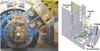 |
Fig. 1 Left: GREAT mounted to the instrument flange, in stow position (the telescope parks at 40° elevation). During observations GREAT (together with the counterweight at top right) rotates ±20° from the vertical. Right: basic structural components of GREAT. One of the two cryostats, the location of the LO compartments and position of the main optics benches are shown. A more detailed view of the optical layout is given in Fig. 2. |
The development of GREAT1 with SOFIA, initially began in 2000, not least as pathfinder for the Herschel satellite mission.
Owing to severe SOFIA project delays, it was not until October 2010, however, that the instrument was shipped to the NASA Dryden Aircraft Operations Facility (DAOF) in Palmdale, CA. On SOFIA’s base there, integration into the aircraft and on-ground commissioning proceeded notably smooth, and first light was recorded already on April 1, 2011, during SOFIA’s observatory characterization flight OCF#4. Since then, GREAT has been operated for more than a dozen flights in SOFIA’s Basic Science program. As a PI-class instrument GREAT is operated by the consortium only, but by agreement with the SOFIA director the instrument has been made available to the SOFIA communities on a collaborative basis.
In the following we focus mainly on the configuration and performance of the instrument as flown during the Short and Basic Science periods of SOFIA. A more detailed technical description of GREAT, including ongoing developments, will be published elsewhere (Heyminck et al., in prep.).
2. Science requirements
The users’ desire for wide radio frequency (RF) coverage (1–5 THz), with highest possible intermediate frequency (IF) bandwidth (>3 GHz) and spectral resolution (<100 kHz) is confronted with current limitations of THz technologies. Despite impressive advances during recent years, the operating bandwidth of the local oscillator (LO) sources in particular is Δν/ν ~ 0.1 only (and significantly less above 2 THz). Therefore, from the beginning (Güsten et al. 2000) GREAT was designed as a highly modular instrument: within the framework of a common infrastructure a choice of two frequency-specific channels can be operated simultaneously. For Early Science three detector channels with a total of four LO sources were flown (Table 1), two more are being developed. The instrument configuration can be changed between flights, while GREAT stays installed on SOFIA.
Science opportunities with GREAT.
3. Instrument description
GREAT is composed of a wide variety of common modules out of which, the desired flight configuration set-up is formed together with the frequency specific subunits (Heyminck et al. 2008).
The mechanical support structure of GREAT (consisting of lightweight, certified aluminum Al-2024 plates) is connected to the science instrument flange of the telescope (Fig. 1). This frame carries the optics box with the common and channel-specific optical components to guide the signals from sky and from the LOs to the mixers. The receiver cryostats and the calibration unit are clamped to the upper side of the structure with tight tolerance, which allows a reproducible re-positioning of the units when the instrument configuration is changed.
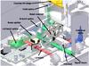 |
Fig. 2 Optics layout: a central polarizer inside the optics compartment splits and re-directs the incoming radiation to the two optics plates of the instrument. A common beam scanning mechanism (for internal alignment) and the calibration loads complete the optical system. |
The structure carries the front-end control electronics on the forward side and the two LOs underneath the optics box (Fig. 1). The optics compartment represents the pressure boundary to the aircraft, is open toward the telescope cavity and hence operates at ambient pressure to minimize absorption losses. The FIR windows maintain the LO compartments at ambient pressure. The total mass of the main structure, including the cryostats, is between 400 and 500 kg, depending on the actual instrument configuration.
Parts of the IF processor and the digital spectrometer back-ends are located in the co-rotating counterweight rack. The so-called PI-rack mounted to the aircraft cabin floor holds the main IF-processor, the acusto-optical spectrometer (AOS) and the chirp transform spectrometer (CTS) back-ends, the power distribution, and the observing computer with ethernet hub.
All GREAT channels flown during Early Science used the same type of liquid nitrogen and liquid helium-cooled cryostat with a similar wiring scheme. Special attention was given to potential safety hazards, and detailed structural analysis was performed. Eight identical units were manufactured so far (Cryovac, Germany), including those assigned for the high-frequency channel. Hold times of 20+ h are adequate for science flights of not more than 10–11 h duration – typically a last top-up is performed four hours before take-off.
These channels all use waveguide-coupled hot-electron bolometers (HEB) as mixing elements, manufactured by KOSMA (see Pütz et al. 2012). Devices are operated at <4.5 K, followed by a cryogenic amplifier (CITLF4, CalTech) without intermediate isolator. All channels work in double-sideband mode. For the calibration a signal-to-image band ratio of 1 is used. Solid-state cascading multiplier chains from Virginia Diodes, Inc., serve as LO reference (Crowe et al. 2011), with commercial synthesizers in the 10−20 GHz frequency range as driver stages. All channels operate a motor-driven Martin-Puplett interferometer as LO diplexer. The LO-power is adjusted via a rotatable wire grid in front of the diplexer.
3.1. Quasi-optical design
GREAT as a dual-color receiver records two frequencies simultaneously (the two beams must co-align on the sky within a fraction of their beam sizes). Except for mirror curvatures, the two L-band channels share a common design consisting of an ambient temperature optics bench and a monolithic cold optics unit inside the cryostat (Wagner-Gentner 2007). The signal from the telescope is separated into the two frequency channels by means of a beam splitter (polarizer grid). The split beams propagate sideways toward “their” optics plate carrying the Martin-Puplett diplexer for LO combining and a focusing off-axis ellipsoidal mirror behind that defines a second beam waist close to the plane of the cryostat window. The LO beam enters from the bottom of the optics compartment and is redirected by a plane mirror through an LO-attenuator toward the diplexer. Inside the cryostat two more off-axis ellipsoids combined with a flat mirror match the beam to the waist of the corrugated mixer feed horn. The Gaussian optics of the L-channels is designed for a lowest frequency of operation of 1.2 THz (here, optical elements are still sized for beam contours of 5.5 times the waist size).
In view of the tighter tolerances required for operation of the M-channel, the optics layout was changed. Following the beam from the beam-splitter, it first is re-imaged by an ellipsoidal mirror creating a broad intermediate waist of 4.4 mm at the beam-splitter of the following Martin-Puplett interferometer. The large intermediate waist size and the now horizontal orientation of the rooftop mirrors make the design more robust against vibrations and alignment errors. The cold optics only consists of one off-axis mirror, matching the beam directly to the horn antenna of the mixer.
For all channels, the wavelength dependence of the diplexer requires mechanical adjustment of its adjustable stage to sub-μm positioning accuracy (see Sect. 3.4.2, for the implementation).
The L1 channel uses high-density polyethelene (HDPE) windows for the cryostat and the LO window in the optics compartment. Since absorption of the material increases with frequency, we chose anti-reflection grooved silicon windows for the L2- and the M-band channels (Wagner-Gentner et al. 2006).
3.2. IF processors and spectrometers
The GREAT IF system operates two IF-processors with remote-control attenuators and total power detectors, one for the AOS and the CTS, one for the fast-Fourier transform (FFT) spectrometer. They shift the IF band (receiver output) to the input band of the individual spectrometer. Both IFs are equipped with remot-control synthesizers for the internal mixing processes, allowing the position of individual spectrometer bands within the IF band to be adjusted.
GREAT offers different types of back-end spectrometers that provide different resolutions and bandwidths. The wide band AOS offers 2 × 4 × 1 GHz of bandwidth with a resolution (equivalent noise bandwidth, ENBW) of ~1.6 MHz (Horn et al. 1999). The IF-processor is capable of stacking four AOS-bands, thus forming two 4 GHz wide bands. The two CTS, however, only have 220 MHz of bandwidth but a spectral resolution of 56 kHz (Villanueva & Hartogh 2004). The fast advancements in digital signal processing during recent years made it possible to equip GREAT with FFT spectrometers (Klein et al. 2006, 2012): each detector channel is serviced by an AFFT spectrometer with 1.5 GHz instantaneous bandwidth and resolution of 212 kHz (ENBW). In June 2011 the latest technology XFFTS was added to the system, providing 2.5 GHz of bandwidth with a resolution of 88 kHz. For the 2012 observing season, the next XFFTS generation with 64 k channels and hence 44 kHz spectral resolution will be available. All back-ends can be operated in parallel.
3.3. Calibration unit
Because frequent receiver gain calibration is essential for high-quality astronomical data, GREAT hosts an internal calibration unit with two black body radiators, one at liquid nitrogen (cold load) and one at ambient temperature (hot load). The cold load cryostat has a hold time of >15 h. A sliding mechanism close to the telescope’s focal plane re-directs the beam to the cold load, to the hot load, or keeps the aperture clear for the sky signal. Depending on the actual observing condition, reference load measurements are taken every 5–10 min.
Proper calibration of losses through the residual atmosphere at flight altitude requires accurate knowledge of the effective load temperatures (see Guan et al. 2012). Therefore we carefully measured the transmission of the HDPE window of the cold load cryostat with a Fourier transform spectrometer and cross-calibrated these measurements against an external windowless liquid nitrogen cooled load (Fig. 3). With the window transmission known, the effective cold load temperature is then calculated individually for each receiver sideband from the physical load temperature measured by three temperature sensors on the cold absorber cone. The overall temperature uncertainty, dominated by the inaccuracy of the window transmission curve (<5%), is <5 K. This corresponds to an approximately 2.5% intensity calibration uncertainty – much lower then the uncertainties in telescope efficiency (Sect. 6) and in atmospheric calibration (see Guan et al. 2012).
3.4. GREAT receiver control
GREAT uses two independent Linux-based computers to control the front-end and to run the observing software, a server for the observing software, and a VME-system for the main tasks of the front-end control.
The optics control electronics provides the calibration unit controls (drive mechanism, temperature readout) and the two controllers for the diplexer drive systems. This system is computer-controlled via RS232 serial lines. The four-channel bias supply for the HEB detectors and the bias supply for the cold low-noise amplifiers together with the cryostat temperature readout are directly connected to the VME-computer I/O hardware, giving full remote control of the front-end.
3.4.1. Software structure
The software that controls the hardware reflects the modularity of the hardware: to each hardware module that can be software-controlled, an individual software task (server) is assigned. In addition, virtual devices exist for modules without direct hardware counterpart. Toghether, these modules provide all necessary functions to operate GREAT. The individual software tasks are spread within the GREAT computer network and communicate via the UDP-protocol. The full software package can be configured by human readable ASCII text files, which also denote which task is running where. All servers use the same code basis and differ only in their configuration files and the hardware-specific code. A hardware simulator to test the higher level software was realized by exchanging the hardware-specific parts only.
All user interfaces, including the graphical user interface, have been realized in Perl/Tk based on a dedicated Perl macro package. The macro package also gives easy access to the full hardware functions within a script-based language. This allows the user to quickly develop special purpose tasks, e.g., for debugging.
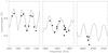 |
Fig. 3 FTS measurements of the cold load window transmission (solid line) and cross calibrations (dots) using an external liquid nitrogen-cooled absorber without window. The two measurements agree well and give confidence in the effective cold load temperature determination, which is important for calibrating the science data accuratly. |
3.4.2. Automatic tuning
Since observing time on an airborne telescope is precious, we have automated the routine operations during observations as much as possible. To change observing frequencies, multiple systems have to be adjusted and re-tuned. For the current GREAT channels we need to set the LO frequency, adjust the LO power level, tune the interferometric diplexer, and level the IF-chain output power. The HEB mixer can be operated on a fixed bias point for all frequencies. Different bias points for the diplexer optimization and for the LO-power adjustment can be chosen.
LO tuning:
the algorithm automatically changes the tuning frequency (following pre-defined procedures to safeguard the hardware) and adjusts its power by measuring the mixer BIAS current at a given point. The optimization is a Newton search using tabulated start values. The L2 channel uses a first incarnation of an electronic LO-power stabilization system. The actual mixer current is kept constant by changing the LO-chain driver amplifier gain. This system also compensates for the direct detection effect (see also below).
Diplexer optimization:
for LO coupling we use Martin-Puplett interferometers in all three channels that are currently in operation. The interferometer is pre-adjusted by calculating a model fit to – previously measured – grid points. This is, if set up well, accurate to better than 5 μm, but an optimum injection of the THz radiation for best noise temperature requires positioning the interferometer to 500 nm accuracy. This final adjustment is made, again relying on a Newton search, by minimizing the total power response (Fig. 4) of the mixer. Setting the LO and tuning the diplexer takes 1–2 min per channel.
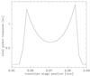 |
Fig. 4 Total power response of the HEB mixer versus diplexer roof top position. The shape of the curve results from decreasing mixer gain with increasing LO pump power (see Pütz et al. 2012, for details). Noise temperature and stability of the system are best at the response minimum. |
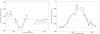 |
Fig. 5 Single-sideband receiver noise temperatures vs. tuning range for bands L1 (left panel) and L2 (right panel). Horizontal lines denote the baseline (dashed lines) and goal performance committed for Early Science. The two curves display average noise temperatures – around the IF-center – for IF bandwidths of 1.0 and 1.5 GHz (higher noise). |
Compensating direct detection:
HEB mixers are known to respond to direct detection (see Pütz et al. 2012), which is the change of the mixer current (and gain) in response to the load by the incoming radiation. Because the effect becomes more prominent with decreasing size of the device, we implemented a correction scheme for the 2.5 THz HEB (this channel showed a noticeable direct-detection effect on the order of 50% in noise temperature, while the lower channels operate with larger devices and showed no measurable effect): after switching to the loads or back to sky we re-adjust the LO power with the optical LO attenuator, and thereby operate the mixer at constant current throughout.
4. Instrument alignment
Rare and expensive flight time together with an estimated turn-around time for optics re-adjustments during flight of >1 h, make it mandatory to ensure proper alignment before flight. The co-alignment between the channels and the optical axis of the telescope is to be established by pre-flight alignment procedures – in the GREAT laboratory at the DAOF and, after installation, in the aircraft. Because of the high athmospheric absorption at sea level, GREAT is blind on sky unless at high flight altitudes, and the determination of the “boresight” offsets to the optical guide cameras can only be performed in flight (once established, the positioning of GREAT toward the astronomical target is defined and maintained by the optical cameras).
In the laboratory, both receiver beams are adjusted to be centered on, and perpendicular to, the instrument mounting flange (consequently also co-aligned). Two beam scanners are used to characterize the beams at two locations, one inside the optics compartment, near the telescope’s focal plane (see Fig. 2), and one at a distance of several meters away from the flange. The reference positions for the beam scanners are defined with a visible laser. Once inside the aircraft, we check that the two beams are well-centered on the secondary mirror by monitoring the total power response of the detectors against cold absorber paddles, but we do not touch their internal alignment. In a last step in flight, the boresight offsets to the guide cameras of SOFIA are determined with pointing scans across a bright planet (that is visible to GREAT and the guide camera, see Fig. 8). The overall pointing accuracy therefore depends on the accuracy of the boresight determination (typically 1–2′′) and the actual co-alignment between the channels (Sect. 6). The stability of the pointing during science operation is controlled with the optical guide cameras to 3–5′′ (in a trade-off between science target integration efficiency and overhead for optical peak-up).
5. GREAT performance during Early Science
GREAT participated in 19 flights, including observatory characterization, commissioning and transfer flights to Europe, during four installation periods. Seven flights (including three for Short Science) were reserved for use by the GREAT consortium, 11 flights assigned for Basic Science community projects on a shared-risk basis; as expected for a new observatory and instrument, not all were successful. Nevertheless, including science data taken during the commissioning flights, a total of 25 science projects were successfully executed.
Three detector channels were operated during Early Science (see Table 1) in the configurations L1a/L2, L1b/L2 and Ma/L2. The successful commissioning of our latest development, the Ma channel operating at 2.5 THz, demonstrates the power of a PI instrument such as GREAT to use state-of-the-art technologies mere weeks after they become available. This capability is unique for SOFIA, as compared to long-planned satellite missions. High-resolution spectroscopy beyond 1.91 THz, above the bands of HIFI on Herschel, is currently only offered by GREAT on SOFIA.
All three GREAT channels show state-of-the-art sensitivity figures combined with a high system stability, allowing for deep integrations and long on-the-fly (OTF) slews. With reference to performance figures presented during the instrument’s pre-shipment review (“baseline”) at many frequencies the sensitivities have improved by factor of 2, some IF bandwidths have been tripled. The 2.5 THz receiver was not even on the horizon at that time. Below we discuss the basic performance figures.
Sensitivities:
Fig. 5 displays single-sideband (SSB) receiver noise temperatures across the RF tuning ranges of the L-band channels. While, fortunately, not impacting at the frequencies of the heavily requested transitions of [CII, 1.90 THz] and [OH, 1.83 THz], increased noise temperatures are recorded in the middle of the L2 band, very likely because of LO noise contributions (a replacement is planed for the 2012 observing season). For the (narrow band) Ma channel the SSB noise temperature (see also Fig. 6) at the OH line is ~7000 K over the usable IF-band of ~900 MHz.
IF bandwidth:
the L-band channels are limited by the mixer roll-off at about 3 GHz and the Martin-Puplett transmission band. For optimum performance with maximized bandwidth we operated at an IF center frequency of 1.625 GHz, with a diplexer center frequency of 1.750 GHz: the higher diplexer frequency partly compensates for the mixer sensitivity roll-off toward higher IF frequencies, while it affects the sensitivity at the lower IF band only negligibly (~5%). The so achieved usable bandwidth is clearly channel-dependent: while for the L1 band a 3 dB noise bandwidth of 1.8 GHz is attainable, the M-band has a bandwidth of 0.9 GHz only (compare Fig. 6). The reason for the limitation in the M-band channel is still under investigation.
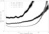 |
Fig. 6 Typical variation of SSB receiver noise temperatures with IF frequency for all three channels. |
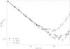 |
Fig. 7 Spectroscopic Allan variance plots for bands L1, L2 and M, calculated between two AFFTS channels separated by 750 MHz. The channel width was set to 850 kHz. |
System stability:
excellent spectroscopic Allan variance minimum times of up to 100 s and longer were measured for the integrated system, while looking at the hot load (Fig. 7). This is excellent for a FIR spectrometer based on HEB detectors, and is the reason for GREAT’s ability to perform long on-the-fly observations with phase times of several 10 s.
5.1. Observing with GREAT
The observing modes supported by GREAT are (1) classical position switching (moving the telescope); (2) beam-switched observations (chopping with the secondary, at a rate of 1–2 Hz), for single-position or raster mapping; and (3) OTF scanning (data are collected while the telescope is slewing across the source). In view of the good stability of the instrument, the OTF mode is most efficient for extended structures, while beam-switching is advised for the observation of weak(er), broad(er) lines toward more compact objects. The wide throw of several arcminutes, with selectable chop direction, is a most valuable asset of the SOFIA chopper.
All Early Science observations were carried out via observing scripts in the environment of the KOSMA-developed kosma_control observing software. For thorough pre-flight testing of the scripts, a realistic stand-alone software simulator is part of this observing package. This simulator was also essential for instrument- and/or telescope-independent software interface testing (toward e.g. the SOFIA Mission Control and Command Software, the front-end or the back-ends).
Almost in real-time, the on-line calibration pipeline displays the science data, which is valuable for real-time decisions. Post-flight, GREAT delivers raw data in modified FITS format into the SOFIA archive, and finally calibrated data (see also Guan et al. 2012) in standard CLASS format, which was adapted to include a SOFIA specific header section.
6. In-flight calibration and efficiencies
By drift scans across bright planets (Saturn in Spring, Jupiter during the Summer flights) we verified the on-sky co-alignment between the two channels that were actually flown, and determined the (common) focus of the instrument. Observations of Mars (size 5.1′′ on Sept. 30) yielded a de-convolved half-power beam width of 21.1″ ± 1″ at 1.337 THz (this frequency is free of terrestrial and Martian atmospheric spectral features), very close to the predicted 21.3′′ for our diffraction-limited optics with a 14 dB edge taper at the subreflector (see Fig. 8). For all flights the pointing of the two channels was co-aligned to better than 4′′.
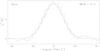 |
Fig. 8 Total power scan of GREAT’s L1-channel tuned to 1.337 THz across Mars. The measured beam is diffraction-limited (fit result shown as dashed line). |
The  calibration scale of GREAT is based on frequent (typically every 10 min) measurements of our integrated hot-cold reference loads. Corrections against atmospheric absorption are performed with the kalibrate-task (Guan et al. 2012) as part of the observing software by spectral fits to the measured sky temperatures across the reception band. The final step to source coupled temperatures, Tmb, requires knowledge of the main-beam coupling efficiencies. On Jupiter and Mars we determined ηmb ~ 0.54 (at 1.3 THz), 0.51 (1.9 THz) and 0.58 (2.5 THz), with estimated 10% uncertainties. This comparatively low throughput is mainly due to the large aperture blockage by the tertiary and the oversized scatter cone at the subreflector. Accumulating only these quantifiable losses (plus blockage through the spiders and the dichroic and reflection losses) we calculated upper limits to the beam efficiencies of 0.56, 0.57 and 0.59, respectively – only slightly higher than what has actually been observed. The differences are attributed to “unspecified losses” such as spill-over, wavefront errors, or optical imperfections (misalignments, incorrect foci).
GREAT performance (during Basic Science).
7. Conclusions and outlook
With GREAT a state-of-the-art dual-color heterodyne receiver for operation onboard of SOFIA has been developed that already during its first observing cycles provided fascinating new insights into the far-infrared universe. The scientific impact is already clearly evident by the large number of scientific contributions to the A&A special feature, which is dedicated to Early Science with GREAT/SOFIA.
The consortium intends to maintain GREAT at the leading edge of THz technologies. GREAT will be continuously upgraded with new opportunities as they become available, improving the performance of existing frequency channels and adding new bands – thereby providing better sensitivities, increasingly wider RF coverage and IF bandwidth to our users. In preparation for Cycle 1, new LO sources will be integrated (band L2, M), including our novel photonic local oscillators, and improved HEB devices will be manufactured (L2, M). New frequency channels (Mb, H) will become available and the FFT spectrometers will then be upgraded to 64 k channels (44 kHz resolution). Once successfully commissioned, the improved GREAT will be available again to the interested SOFIA communities in collaboration with the consortium (following conditions similar to those implemented for Basic Science).
Since last summer upGREAT is on course – a parallel development to the improvements of the existing channels that building on the infrastructure of GREAT, aims at delivering two compact heterodyne detector arrays with 2 × 7 pixels (1.9–2.5 THz) and 1 × 7 pixel (4.7 THz), respectively. Within an ambitious schedule, we aim at commissioning the first of the low-frequency sub-arrays in Cycle 2.
GREAT is a development by the MPI für Radioastronomie (Principal Investigator: R. Güsten) and the KOSMA/Universität zu Köln, in cooperation with the MPI für Sonnensystemforschung and the DLR Institut für Planetenforschung.
Acknowledgments
During its long development many have contributed to the success of GREAT, too many to be named here. We thank the SOFIA engineering and operations teams, whose tireless support and good-spirit teamwork has been essential for the GREAT accomplishments during Early Science. Herzlichen Dank to the DSI telescope engineering team. Finally, we thank the Project Management for bringing SOFIA back on schedule! IRAM/GRENOBLE has implemented the GREAT/SOFIA specific CLASS header extensions. SOFIA Science Mission Operations are conducted jointly by the Universities Space Research Association, Inc., under NASA contract NAS2-97001, and the Deutsches SOFIA Institut under DLR contract 50 OK 0901. The development of GREAT was financed by the participating institutes, the Max-Planck-Society, and the German Research Society within the framework of SFB 494.
References
- Becklin, E. E., & Gehrz, R. D. 2009, in Submillimeter Astrophysics and Technology: a Symposium Honoring Thomas G. Phillips, ASP Conf. Ser., 417, 101 [NASA ADS] [Google Scholar]
- Betz, A., & Zmuidzinas, J. S. 1984, in Airborne Astronomy Symposium, 320 [Google Scholar]
- Crowe, T. W., Hesler, J. L., Retzloff, S. A., Pouzou, C., & Schoenthal, G. S. 2011, in 22nd Int. Symp. on Space Terahertz Technology [Google Scholar]
- de Graauw, T., Helmich, F. P., Phillips, T. G., et al. 2010, A&A, 518, L6 [NASA ADS] [CrossRef] [EDP Sciences] [Google Scholar]
- Gillespie, Jr., C. M. 1981, in SPIE Conf. Ser., 265, 1 [Google Scholar]
- Guan, X., Stutzki, J., Graf, U., et al. 2012, A&A, 542, L4 [Google Scholar]
- Güsten, R., Hartogh, P., Huebers, H.-W., et al. 2000, in SPIE Conf. Ser., 4014, 23 [Google Scholar]
- Heyminck, S., Güsten, R., Hartogh, P., et al. 2008, in SPIE Conf. Ser., 7014 Part 1, 701410 [Google Scholar]
- Horn, J., Siebertz, O., Schmülling, F., et al. 1999, Exper. Astron., 9, 17 [Google Scholar]
- Klein, B., Philipp, S. D., Krämer, I., et al. 2006, A&A, 454, L29 [NASA ADS] [CrossRef] [EDP Sciences] [Google Scholar]
- Klein, B., Hochgürtel, S., Krämer, I., et al. 2012, A&A, 542, L3 [NASA ADS] [CrossRef] [EDP Sciences] [Google Scholar]
- Phillips, T. G. 1981, in SPIE Conf. Ser., 280, 101 [Google Scholar]
- Pilbratt, G. L., Riedinger, J. R., Passvogel, T., et al. 2010, A&A, 518, L1 [CrossRef] [EDP Sciences] [Google Scholar]
- Pütz, P., Honingh, C. E., Jacobs, K., et al. 2012, A&A, 542, L2 [NASA ADS] [CrossRef] [EDP Sciences] [Google Scholar]
- Röser, H. P., Schäfer, F., Schmid-Burgk, J., Schultz, G. V., & van der Wal, P. 1987, International Journal of Infrared and Millimeter Waves, 8, 1541 [NASA ADS] [CrossRef] [Google Scholar]
- Villanueva, G., & Hartogh, P. 2004, Exper. Astron., 18, 77 [Google Scholar]
- Wagner-Gentner, A. 2007, Ph.D. Thesis, University of Cologne, Germany [Google Scholar]
- Wagner-Gentner, A., Graf, U., Rabanus, D., & Jacobs, K. 2006, Infrared Physics & Technology, 48, 249 [NASA ADS] [CrossRef] [Google Scholar]
- Young, E. T., Becklin, E. E., Marcum, P. M., et al. 2012, ApJ, 749, L17 [NASA ADS] [CrossRef] [Google Scholar]
All Tables
All Figures
|
Fig. 1 Left: GREAT mounted to the instrument flange, in stow position (the telescope parks at 40° elevation). During observations GREAT (together with the counterweight at top right) rotates ±20° from the vertical. Right: basic structural components of GREAT. One of the two cryostats, the location of the LO compartments and position of the main optics benches are shown. A more detailed view of the optical layout is given in Fig. 2. |
| In the text | |
|
Fig. 2 Optics layout: a central polarizer inside the optics compartment splits and re-directs the incoming radiation to the two optics plates of the instrument. A common beam scanning mechanism (for internal alignment) and the calibration loads complete the optical system. |
| In the text | |
|
Fig. 3 FTS measurements of the cold load window transmission (solid line) and cross calibrations (dots) using an external liquid nitrogen-cooled absorber without window. The two measurements agree well and give confidence in the effective cold load temperature determination, which is important for calibrating the science data accuratly. |
| In the text | |
|
Fig. 4 Total power response of the HEB mixer versus diplexer roof top position. The shape of the curve results from decreasing mixer gain with increasing LO pump power (see Pütz et al. 2012, for details). Noise temperature and stability of the system are best at the response minimum. |
| In the text | |
|
Fig. 5 Single-sideband receiver noise temperatures vs. tuning range for bands L1 (left panel) and L2 (right panel). Horizontal lines denote the baseline (dashed lines) and goal performance committed for Early Science. The two curves display average noise temperatures – around the IF-center – for IF bandwidths of 1.0 and 1.5 GHz (higher noise). |
| In the text | |
|
Fig. 6 Typical variation of SSB receiver noise temperatures with IF frequency for all three channels. |
| In the text | |
|
Fig. 7 Spectroscopic Allan variance plots for bands L1, L2 and M, calculated between two AFFTS channels separated by 750 MHz. The channel width was set to 850 kHz. |
| In the text | |
|
Fig. 8 Total power scan of GREAT’s L1-channel tuned to 1.337 THz across Mars. The measured beam is diffraction-limited (fit result shown as dashed line). |
| In the text | |
Current usage metrics show cumulative count of Article Views (full-text article views including HTML views, PDF and ePub downloads, according to the available data) and Abstracts Views on Vision4Press platform.
Data correspond to usage on the plateform after 2015. The current usage metrics is available 48-96 hours after online publication and is updated daily on week days.
Initial download of the metrics may take a while.