| Issue |
A&A
Volume 541, May 2012
|
|
|---|---|---|
| Article Number | A84 | |
| Number of page(s) | 5 | |
| Section | Cosmology (including clusters of galaxies) | |
| DOI | https://doi.org/10.1051/0004-6361/201118130 | |
| Published online | 03 May 2012 | |
Research Note
A brief analysis of self-gravitating polytropic models with a non-zero cosmological constant
1
University of Rome “La Sapienza”Department of Physics,
Piazzale Aldo Moro 2,
00185
Rome,
Italy
e-mail: This email address is being protected from spambots. You need JavaScript enabled to view it.
2
Space Research Institute (IKI) Profsoyuznaya 84/32,
117997
Moscow,
Russia
e-mail: This email address is being protected from spambots. You need JavaScript enabled to view it.
3
National Research Nuclear University MEPHI,
Kashirskoe Shosse
31, 115409
Moscow,
Russia
e-mail: This email address is being protected from spambots. You need JavaScript enabled to view it.
Received:
21
September
2011
Accepted:
24
February
2012
Abstract
Context. We investigate the equilibrium and stability of polytropic spheres in the presence of a non-zero cosmological constant.
Aims. We solve the Newtonian gravitational equilibrium equation for a system with a polytropic equation of state of the matter P = Kργ introducing a non-zero cosmological constant Λ.
Methods. We consider the cases of n = 1, 1.5, 3 and construct series of solutions with a fixed value of Λ. For each value of n, the non-dimensional equilibrium equation has a family of solutions, instead of the unique solution of the Lane-Emden equation at Λ = 0.
Results. The equilibrium state exists only for central densities ρ0 higher than the critical value ρc. There are no static solutions at ρ0 < ρc. We investigate the stability of equilibrium solutions in the presence of a non-zero Λ and show that dark energy reduces the dynamic stability of the configuration. We apply our results to the analysis of the properties of the equilibrium states of clusters of galaxies in the present universe with non-zero Λ.
Key words: dark matter / dark energy / galaxies: clusters: general
© ESO, 2012
1. Introduction
Detailed analysis of the observations of distant SN Ia (Riess et al. 1998; Perlmutter et al. 1999) and the spectrum of fluctuations in the cosmic microwave background radiation (CMB) (see e.g. Spergel et al. 2003) have lead to the conclusion that the term representing “dark energy” (DE) contains about 70% of the average energy density in the present universe and its properties are very close (identical) to the properties of the Einstein cosmological Λ term. In the papers of Chernin (see review 2008), the question was raised about the possible influence of any cosmological constant on the properties of the Hubble flow in the local galaxy cluster (LC) and whether the LC can exist in the equilibrium state, at present values of the DE density, where the LC densities of matter consist of the baryonic and dark matter.
Here, we construct Newtonian self-gravitating models with a polytropic equation of state in the presence of DE. In this case, we have a family instead of the single model for each polytropic index n. The additional parameter β represents the ratio of the density of DE to the matter central density of the configuration. For values of n = 1, 1.5, 3, corresponding to the polytropic powers γ = 2, 5/3, 4/3, we find the limiting values of βc, such that at β > βc there are no equilibrium configurations but only an expanding cluster, possibly affected by the Hubble flow.
We derive a virial theorem and analyze the influence of DE on the dynamic stability of the equilibrium models, by using an approximate energetic method. It is shown that DE produces an effect that counteracts the stabilizing influence of the cold dark matter (McLaughlin & Fuller 1996; Bisnovatyi-Kogan 1998).
2. Main equations
We consider a spherically symmetric equilibrium configuration in Newtonian gravity, in the
presence of DE, represented by the cosmological constant Λ. In this case, the gravitational
force Fg that a unit mass undergoes in a spherically symmetric
body is written as  , where
m = m(r) is the mass inside the radius
r. Its connections with the matter density ρ and the
equilibrium equation are written respectively as
, where
m = m(r) is the mass inside the radius
r. Its connections with the matter density ρ and the
equilibrium equation are written respectively as 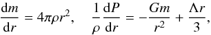 (1)and the DE density
ρv is connected with Λ as
(1)and the DE density
ρv is connected with Λ as
 .
We consider a polytropic equation of state
P = Kργ,
with
.
We consider a polytropic equation of state
P = Kργ,
with  . By
introducing the non-dimensional variables ξ and
θn such that
. By
introducing the non-dimensional variables ξ and
θn such that 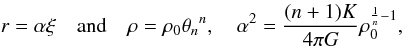 (2)we obtain the
Lane-Emden equation for polytropic models with DE (see also Balaguera-Antolínez et al. 2007)
(2)we obtain the
Lane-Emden equation for polytropic models with DE (see also Balaguera-Antolínez et al. 2007) 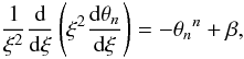 (3)where
ρ0 is the matter central density, α is the
characteristic radius, and
β = Λ/4πGρ0 = 2ρv/ρ0
is twice the ratio of the DE density to the central density of the configuration.
(3)where
ρ0 is the matter central density, α is the
characteristic radius, and
β = Λ/4πGρ0 = 2ρv/ρ0
is twice the ratio of the DE density to the central density of the configuration.
3. The virial theorem
We first calculate the Newtonian gravitational energy of the configuration in the presence
of the cosmological constant. The spherically symmetric Poisson equation for the
gravitational potential ϕ∗ in the presence of DE is given by
 (4)The gravitational energy of
a spherical body εg is given by
(4)The gravitational energy of
a spherical body εg is given by 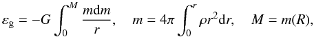 (5)where R is
the total radius. For ϕΛ with uniform density
ρv the normalization ϕ = 0
at r = ∞ is impossible. We can then choose
ϕΛ = 0 at r = 0 as the most convenient
normalization. This choice, using Eq. (4),
leads to the potential
ϕΛ = −4πGρvr2/3.
Consequently, the energy εΛ, representing the interaction of the
matter with DE, is given by
(5)where R is
the total radius. For ϕΛ with uniform density
ρv the normalization ϕ = 0
at r = ∞ is impossible. We can then choose
ϕΛ = 0 at r = 0 as the most convenient
normalization. This choice, using Eq. (4),
leads to the potential
ϕΛ = −4πGρvr2/3.
Consequently, the energy εΛ, representing the interaction of the
matter with DE, is given by 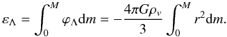 (6)We find the relations
between the gravitational εg and thermal
εth energies, and the energy εΛ.
For the gravitational energy, we have
(6)We find the relations
between the gravitational εg and thermal
εth energies, and the energy εΛ.
For the gravitational energy, we have 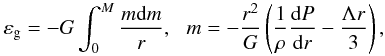 (7)where
M = m(R), and m is
written using Eq. (1). For adiabatic systems
with a polytropic equation of state, we have ρE = nP and
(7)where
M = m(R), and m is
written using Eq. (1). For adiabatic systems
with a polytropic equation of state, we have ρE = nP and
 , where E and
I are thermal energy and enthalpy per mass unit. After some
transformations, we obtain
, where E and
I are thermal energy and enthalpy per mass unit. After some
transformations, we obtain 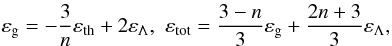 (8)where
εtot = εth + εg + εΛ,
(8)where
εtot = εth + εg + εΛ,
 , while
 is
defined by Eq. (6), and the additive constant
in the energy definition of εΛ is chosen so that
εΛ = 0 at Λ = 0 or M = 0. The gravitational
energy may also be written as
is
defined by Eq. (6), and the additive constant
in the energy definition of εΛ is chosen so that
εΛ = 0 at Λ = 0 or M = 0. The gravitational
energy may also be written as 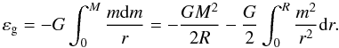 (9)We can transform the last
integral for polytropic matter by using Eq. (7) and making partial integrations. We have
(9)We can transform the last
integral for polytropic matter by using Eq. (7) and making partial integrations. We have 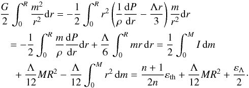 (10)Then,
by using Eqs. (8) and (10), we obtain from Eq. (9) the relations
(10)Then,
by using Eqs. (8) and (10), we obtain from Eq. (9) the relations 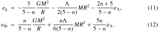 Finally,
by inserting Eq. (12) into (8), we get
Finally,
by inserting Eq. (12) into (8), we get 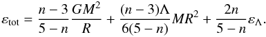 (13)We can calculate
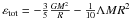
εtot for some particular cases. For
n = 3, 1, and 0, we
have, respectively,
(13)We can calculate
εtot for some particular cases. For
n = 3, 1, and 0, we
have, respectively,  , and
, and
 . The Lane-Emden model
with n = 5 has an analytical solution with finite mass M,
finite values of the energies, and an infinite radius R, so that must be
(5 − n)R → constant (const.) at n → 5.
In the presence of DE, the finiteness of values of all kinds of energies requires that
. The Lane-Emden model
with n = 5 has an analytical solution with finite mass M,
finite values of the energies, and an infinite radius R, so that must be
(5 − n)R → constant (const.) at n → 5.
In the presence of DE, the finiteness of values of all kinds of energies requires that
 The
Lane-Emden solution (without DE) at n = 3 has zero total energy at any
given radius and corresponds to a neutral equilibrium. Hence, the knowledge of the total
energy of the configuration permits us to identify the boundary between dynamically stable
(n < 3,
εtot < 0) and unstable
(n > 3,
εtot > 0) configurations. In our case,
the virial theorem does not permit us to do this, because the value of
εΛ is not properly defined, while the presence of DE in the
whole space does not permit us to choose, in a simple way, a universal additive constant of
the energy. Therefore, in spite of
εtot = 3εΛ < 0
at n = 3 and in accordance with the stability analysis made in Sect. 4, the
polytropic solution at n = 3 in the presence of DE becomes unstable. Some
aspects of the virial theorem in the presence of Λ were investigated by Balaguera-Antolínez
et al. (2007).
The
Lane-Emden solution (without DE) at n = 3 has zero total energy at any
given radius and corresponds to a neutral equilibrium. Hence, the knowledge of the total
energy of the configuration permits us to identify the boundary between dynamically stable
(n < 3,
εtot < 0) and unstable
(n > 3,
εtot > 0) configurations. In our case,
the virial theorem does not permit us to do this, because the value of
εΛ is not properly defined, while the presence of DE in the
whole space does not permit us to choose, in a simple way, a universal additive constant of
the energy. Therefore, in spite of
εtot = 3εΛ < 0
at n = 3 and in accordance with the stability analysis made in Sect. 4, the
polytropic solution at n = 3 in the presence of DE becomes unstable. Some
aspects of the virial theorem in the presence of Λ were investigated by Balaguera-Antolínez
et al. (2007).
4. Equilibrium solutions
The equilibrium mass Mn for a generic
polytropic configuration that is a solution of the Lane-Emden equation is written as
![Mathematical equation: \begin{equation} M_n=4\pi \!\int_0^{R}\!\rho r^2 {\rm d}r\!=\!4\pi \left[\frac{(n\!+\!1)K}{4\pi G}\right]^{3/2}\rho_0^{\frac{3}{2n}-\frac{1}{2}}\! \int_0^{\xi_{\rm out}}\!{\theta_n}^n\xi^2 {\rm d}\xi. \label{eq13} \end{equation}](/articles/aa/full_html/2012/05/aa18130-11/aa18130-11-eq78.png) (14)Using Eq. (3), the integral on the right side may be
calculated by partial integration, giving the relation for the mass of the configuration
(14)Using Eq. (3), the integral on the right side may be
calculated by partial integration, giving the relation for the mass of the configuration
![Mathematical equation: \begin{equation} M_n=4\pi \rho_0 \alpha^3\left[-\xi_{\rm out}^2\left(\frac{{\rm d}\theta_n}{{\rm d}\xi}\right)_{\rm out}+ \frac{\beta\xi_{\rm out}^3}{3}\right], \label{eq15} \end{equation}](/articles/aa/full_html/2012/05/aa18130-11/aa18130-11-eq79.png) (15)where
θn(ξ) is not a unique
function, but depends on the parameter β, according to Eq. (3). For the limiting configuration, with
β = βc, we have on the outer boundary
(15)where
θn(ξ) is not a unique
function, but depends on the parameter β, according to Eq. (3). For the limiting configuration, with
β = βc, we have on the outer boundary
 , and the mass
Mn,lim of the limiting configuration is
written as
, and the mass
Mn,lim of the limiting configuration is
written as 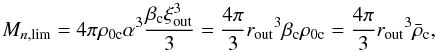 (16)such that the limiting
value βc is exactly equal to the ratio of the average matter
density
(16)such that the limiting
value βc is exactly equal to the ratio of the average matter
density  of the limiting configuration to its central density ρ0c:
 .
For the Lane-Emden solution (with β = 0), we have
.
For the Lane-Emden solution (with β = 0), we have
 for n = 1, 1.5, 3,
respectively. We consider the curve M(ρ0) for a
constant DE density
ρv = Λ/8πG.
In order to plot this curve in the non-dimensional form, we introduce an arbitrary scaling
constant ρch and write the expression for the mass in the form
for n = 1, 1.5, 3,
respectively. We consider the curve M(ρ0) for a
constant DE density
ρv = Λ/8πG.
In order to plot this curve in the non-dimensional form, we introduce an arbitrary scaling
constant ρch and write the expression for the mass in the form
![Mathematical equation: \hbox{$M_n=4\pi \left[\frac{(n+1)K}{4\pi G}\right]^{3/2}\rho_{\rm ch}^{\frac{3}{2n} -\frac{1}{2}}{\hat M_n},$}](/articles/aa/full_html/2012/05/aa18130-11/aa18130-11-eq93.png) with
with ![Mathematical equation: \begin{equation} {\hat M_n}=\hat\rho_0^{\frac{3}{2n}-\frac{1}{2}} \left[\frac{\beta\xi_{\rm out}^3}{3}-\xi_{\rm out}^2 \left(\frac{{\rm d}\theta_n}{{\rm d}\xi}\right)_{\rm out}\right], \label{eq20} \end{equation}](/articles/aa/full_html/2012/05/aa18130-11/aa18130-11-eq94.png) (17)where
(17)where
 is the non-dimensional central density. We also introduced the non-dimensional mass
 .
.
At n = 1, Eq. (3) is linear
and has an analytic solution (Chandrasekhar 1939). The
solution satisfying the boundary conditions at the center,
θ1(0) = 1, θ1′(0) = 0, is
written as 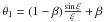 . The radius of the configuration
is determined by the transcendental equation
. The radius of the configuration
is determined by the transcendental equation 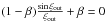 . This equation only has real
solutions at β < βc,
such that at the outer boundary not only does θ1 = 0, but also
θ1′ = 0 for
β = βc. We have
. This equation only has real
solutions at β < βc,
such that at the outer boundary not only does θ1 = 0, but also
θ1′ = 0 for
β = βc. We have
 .
Therefore, the parameters βc and
ξout,c of the limiting equilibrium solution
in the presence of DE are determined by the algebraic equations
.
Therefore, the parameters βc and
ξout,c of the limiting equilibrium solution
in the presence of DE are determined by the algebraic equations
 and
tanξout,c = ξout,c,
where
π < ξout,c < 3π/2.
At large ξ, the solutions asymptotically approach the horizontal line
θ1 = β. Our numerical analysis indicates that
ξout = π, 3.490, 4.493,
for
β = 0, β = 0.5βc = 0.089,
and β = βc = 0.178, respectively. We plot the
non-dimensional curve
and
tanξout,c = ξout,c,
where
π < ξout,c < 3π/2.
At large ξ, the solutions asymptotically approach the horizontal line
θ1 = β. Our numerical analysis indicates that
ξout = π, 3.490, 4.493,
for
β = 0, β = 0.5βc = 0.089,
and β = βc = 0.178, respectively. We plot the
non-dimensional curve  ,
at constant
ρv = βρ0/2.
We construct the curve starting from the model with
,
at constant
ρv = βρ0/2.
We construct the curve starting from the model with  at different β, and then following the sequence by varying the central
density
at different β, and then following the sequence by varying the central
density  assuming that
  ,
at β ≤ βc. For n = 1, we have
,
at β ≤ βc. For n = 1, we have
![Mathematical equation: \begin{equation} \hat M_1=\hat\rho_0\left[(1-\beta)(\sin\xi_{\rm out}-\xi_{\rm out}\cos\xi_{\rm out}) + \frac{\beta \xi_{\rm out}^3}{3}\right],\quad \label{eq22} \end{equation}](/articles/aa/full_html/2012/05/aa18130-11/aa18130-11-eq120.png) (18)where
(18)where
 .
The behavior of
.
The behavior of  is given in Fig. 1 for
βin = 0, βin = 0.5βc,
and βin = βc, for which
is given in Fig. 1 for
βin = 0, βin = 0.5βc,
and βin = βc, for which
 at .
We note that for βin = βc there are
equilibrium models only for
at .
We note that for βin = βc there are
equilibrium models only for  .
.
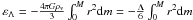
 |
Fig. 1 Non-dimensional mass |

At n = 3, the mass of the configuration is given by
![Mathematical equation: \hbox{$ M_3=4\pi \left[\frac{K}{\pi G}\right]^{3/2}{\hat M_3}$}](/articles/aa/full_html/2012/05/aa18130-11/aa18130-11-eq130.png) ,
where
,
where  is derived by Eq. (17). The Lane-Emden model
(β = 0) has a unique value of the mass that is independent of the density
(equilibrium configuration with neutral dynamical stability). At β ≠ 0, the
model’s dependence on the density appears because the function
θ3 is different for different values of β
and, along the curve
is derived by Eq. (17). The Lane-Emden model
(β = 0) has a unique value of the mass that is independent of the density
(equilibrium configuration with neutral dynamical stability). At β ≠ 0, the
model’s dependence on the density appears because the function
θ3 is different for different values of β
and, along the curve  ,
the value of β is inversely proportional to
.
,
the value of β is inversely proportional to
.
The density distribution for equilibrium configurations with
β = 0, β = 0.5βc,
and β = βc is shown in Fig. 2. At large ξ, these solutions
asymptotically approach the horizontal line
θ3 = β1/3, with
damping oscillations around this value. The numerical solution of the equilibrium equation
gives
ξout = 6.897, 7.489, 9.889,
for
β = 0, β = 0.5βc = 0.003,
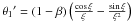
and β = βc = 0.006, respectively. In Fig. 3, we show the behavior of
,
for different values of
βin = 0, βin = 0.5βc,
and βin = βc, for which
 ,
at ,
respectively.
,
at ,
respectively.
 |
Fig. 2 The density distribution for configurations at n = 3 with β = 0, β = 0.5βc, and β = βc. The curves are marked with the values of β. The non-physical solution at β = 1.5βc, which does not have an outer boundary, is given by the dash-dot line. The non-physical parts of the solutions at β ≤ βc, behind the outer boundary, are given by the dash lines. The solutions asymptotically approach, at large ξ, the horizontal line θ3 = β1/3. |
The behavior of  in Fig. 3, showing a decreasing mass with increasing
central density, corresponds, for an adiabatic index equal to the polytropic one, to
dynamically unstable configurations, according to the static criterion of stability
(Zel’dovich 1963). When the vacuum influence is
small, it is possible to investigate the stability of the adiabatic configuration by the
approximate energetic method (Zeldovich & Novikov 1966; Bisnovatyi-Kogan 2001). For n = 3, at
ρ0 ≫ ρv, the
density in the configuration is distributed according to the Lane-Emden solution
in Fig. 3, showing a decreasing mass with increasing
central density, corresponds, for an adiabatic index equal to the polytropic one, to
dynamically unstable configurations, according to the static criterion of stability
(Zel’dovich 1963). When the vacuum influence is
small, it is possible to investigate the stability of the adiabatic configuration by the
approximate energetic method (Zeldovich & Novikov 1966; Bisnovatyi-Kogan 2001). For n = 3, at
ρ0 ≫ ρv, the
density in the configuration is distributed according to the Lane-Emden solution
 . In this case, we may
investigate the stability to homologous perturbations by changing only the central density
at fixed density distribution, given by the function θ3.
. In this case, we may
investigate the stability to homologous perturbations by changing only the central density
at fixed density distribution, given by the function θ3.
We consider configurations close to the polytropic (adiabatic) equilibrium solution at
n = 3 (and β = 0), where the turning point of stability
is expected. In this case, the presence of DE does not affect significantly the
gravitational equilibrium, thus the unperturbed polytropic solution at
n = 3 can be used to calculate the gravitational energy
εg. The energy ε∗ will then be
given by  (19)thus
 , where,
taking into account the non-dimensional variables in Eq. (2), the energy εΛ can be written as
, where,
taking into account the non-dimensional variables in Eq. (2), the energy εΛ can be written as
 (20)where
 (see Bisnovatyi-Kogan 2001). In the analysis of the dynamical stability, we
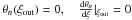
consider the total energy ε of the configuration, taking into account a
small correction εGR due to general relativistic effects. We
have
(see Bisnovatyi-Kogan 2001). In the analysis of the dynamical stability, we
consider the total energy ε of the configuration, taking into account a
small correction εGR due to general relativistic effects. We
have  (21)where
we used the relations for the polytropic configuration with n = 3,
ξout = 6.897, and
(21)where
we used the relations for the polytropic configuration with n = 3,
ξout = 6.897, and 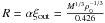 . The
equilibrium configuration is determined by the zero of the first derivative of
ε over ρ0, at constant entropy
S and mass M, while the stability of the configuration
is analyzed in terms of the sign of the second derivative: if positive, the configuration is
dynamically stable, if negative, the configuration is unstable. It is more convenient to
take derivatives over
. The
equilibrium configuration is determined by the zero of the first derivative of
ε over ρ0, at constant entropy
S and mass M, while the stability of the configuration
is analyzed in terms of the sign of the second derivative: if positive, the configuration is
dynamically stable, if negative, the configuration is unstable. It is more convenient to
take derivatives over  than over ρ0. Thus
 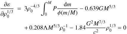 (22)for
the equilibrium, and the sign of the second derivative
(22)for
the equilibrium, and the sign of the second derivative  (23)for
the analysis of the dynamical stability, where
(23)for
the analysis of the dynamical stability, where  and
and
 are the adiabatic index γ at constant entropy S and the
non-dimensional function φ, which both remain constant during homologous
perturbations, respectively. It follows from Eq. (23) that DE input in the stability of the configuration is negative, as in the
general relativistic correction (Chandrasekhar 1964;
Merafina & Ruffini 1989). Therefore, an
adiabatic star with a polytropic index of 4/3 becomes unstable in the
presence of DE. The dynamic stability of pure polytropic models was also investigated by
Balaguera-Antolínez et al. (2006, 2007), by using a static criterion of stability. Our
criterion is valid for any equation of state P(ρ,T).
are the adiabatic index γ at constant entropy S and the
non-dimensional function φ, which both remain constant during homologous
perturbations, respectively. It follows from Eq. (23) that DE input in the stability of the configuration is negative, as in the
general relativistic correction (Chandrasekhar 1964;
Merafina & Ruffini 1989). Therefore, an
adiabatic star with a polytropic index of 4/3 becomes unstable in the
presence of DE. The dynamic stability of pure polytropic models was also investigated by
Balaguera-Antolínez et al. (2006, 2007), by using a static criterion of stability. Our
criterion is valid for any equation of state P(ρ,T).
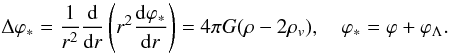
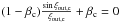
At n = 1.5, the mass of the configuration is written as
![Mathematical equation: \hbox{$M_{3/2}=4\pi \left[\frac{5K}{8\pi G}\right]^{3/2}\rho_{\rm ch}^{1/2}{\hat M_{3/2}}$}](/articles/aa/full_html/2012/05/aa18130-11/aa18130-11-eq169.png) ,
where
,
where  is derived by Eq. (17). At large
ξ, these solutions asymptotically approach the horizontal line
θ3/2 = β2/3.
The numerical solution gives
ξout = 3.654, 3.984, 5.086,
for
β = 0, β = 0.5βc = 0.041, β = βc = 0.082,
respectively. In Fig. 4, we show the behavior of
is derived by Eq. (17). At large
ξ, these solutions asymptotically approach the horizontal line
θ3/2 = β2/3.
The numerical solution gives
ξout = 3.654, 3.984, 5.086,
for
β = 0, β = 0.5βc = 0.041, β = βc = 0.082,
respectively. In Fig. 4, we show the behavior of
 ,
for different values of
βin = 0, βin = 0.5βc,
and βin = βc, for which
,
for different values of
βin = 0, βin = 0.5βc,
and βin = βc, for which
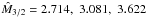 ,
at ,
respectively.
,
at ,
respectively.
5. Discussion
The question about the importance of DE to the dynamics of the Local Cluster (LC) was
raised by Chernin (2008). For presently accepted
values of the DE density
ρv = (0.72 ± 0.03) × 10-29 g/cm3,
the mass of the Local Group, including its dark matter input, is between
MLC ~ 3.5 × 10¹² M⊙,
according to Chernin et al. (2009), and
MLC ~ 1.3 × 10¹² M⊙,
according to Karachentsev et al. (2006). The radius
RLC of the LC is even more poorly known. It can be estimated
by measuring the velocity dispersion vt of galaxies in the LC
and by the application of the virial theorem, such that
 . The estimated velocity
dispersion of galaxies in the LC, which has been found to equal
vt = 63 km s-1, is very close to the value of the
local Hubble constant H = 68 km s-1 Mpc-1
(Karachentsev et al. 2006). The similarity between
these values indicates the great difficulties in dividing the measured velocities between
regular and chaotic components. The radius of the LC may be estimated to be
. The estimated velocity
dispersion of galaxies in the LC, which has been found to equal
vt = 63 km s-1, is very close to the value of the
local Hubble constant H = 68 km s-1 Mpc-1
(Karachentsev et al. 2006). The similarity between
these values indicates the great difficulties in dividing the measured velocities between
regular and chaotic components. The radius of the LC may be estimated to be
 , and to have values between
1.5 Mpc and 4 Mpc and a very large error box that we cannot estimate properly. Chernin
et al. (2009) identifies the radius
RLC with the radius
Rv of the zero-gravity force, which is
identical to the one corresponding to our critical model with
β = βc, in which the average matter density
is equal to 2ρv:
1.2 < MLC < 3.7 × 10¹² M⊙
and
1.1 < Rv < 1.6 Mpc.
All these estimations show the importance of the presently accepted value of DE density on
the structure and dynamics of the outer parts of LC, and its vicinity. Polytropic solutions
with DE are inappropriate for describing the LC, but may be more applicable to rich galactic
clusters.
, and to have values between
1.5 Mpc and 4 Mpc and a very large error box that we cannot estimate properly. Chernin
et al. (2009) identifies the radius
RLC with the radius
Rv of the zero-gravity force, which is
identical to the one corresponding to our critical model with
β = βc, in which the average matter density
is equal to 2ρv:
1.2 < MLC < 3.7 × 10¹² M⊙
and
1.1 < Rv < 1.6 Mpc.
All these estimations show the importance of the presently accepted value of DE density on
the structure and dynamics of the outer parts of LC, and its vicinity. Polytropic solutions
with DE are inappropriate for describing the LC, but may be more applicable to rich galactic
clusters.
Acknowledgments
The work of GSBK and SOT was partially supported by RFBR grant 11-02-00602, the Presidium RAN program P20 and RF President Grant NSh-3458.2010.2.
References
- Balaguera-Antolínez, A., Mota, D. F., & Nowakowski, M. 2006, Class. Quant. Grav., 23, 4497 [NASA ADS] [CrossRef] [Google Scholar]
- Balaguera-Antolínez, A., Mota, D. F., & Nowakowski, M. 2007, MNRAS, 382, 621 [NASA ADS] [CrossRef] [Google Scholar]
- Bisnovatyi-Kogan, G. S. 1998, ApJ, 497, 559 [NASA ADS] [CrossRef] [Google Scholar]
- Bisnovatyi-Kogan, G. S. 2001, Stellar Physics, II. Stellar Structure and Stability (Heidelberg: Springer) [Google Scholar]
- Chandrasekhar, S. 1939, An Introduction to the Study of Stellar Structure (Chicago: Univ. Chicago Press) [Google Scholar]
- Chandrasekhar, S. 1964, ApJ, 140, 417 [NASA ADS] [CrossRef] [MathSciNet] [Google Scholar]
- Chernin, A. D. 2008, Phys. Usp., 51, 267 [Google Scholar]
- Chernin, A. D., Teerikorpi, P., Valtonen, M. J., et al. 2009, ApJL, submitted [arXiv:astro-ph0902.3871v1] [Google Scholar]
- Karachentsev, I. D., Dolphin, A., Tully, R. B., et al. 2006, AJ, 131, 1361 [NASA ADS] [CrossRef] [Google Scholar]
- McLaughlin, G., & Fuller, G. 1996, ApJ, 456, 71 [NASA ADS] [CrossRef] [Google Scholar]
- Merafina, M., & Ruffini, R. 1989, A&A, 221, 4 [NASA ADS] [Google Scholar]
- Perlmutter, S., Aldering, G., Goldhaber, G., et al. 1999, ApJ, 517, 565 [NASA ADS] [CrossRef] [Google Scholar]
- Riess, A. G., Filippenko, A. V., Challis, P., et al. 1998, AJ, 116, 1009 [NASA ADS] [CrossRef] [Google Scholar]
- Spergel, D. N., Verde, L., Peiris, H. V., et al. 2003, ApJS, 148, 175 [NASA ADS] [CrossRef] [Google Scholar]
- Zel’dovich, Ya. B. 1963, Voprosy Kosmogonii, 9, 157 [Google Scholar]
- Zel’dovich, Ya. B., & Novikov, I. D. 1966, Phys. Usp., 8, 522 [NASA ADS] [CrossRef] [Google Scholar]
All Figures
|
Fig. 1 Non-dimensional mass |
| In the text | |
|
Fig. 2 The density distribution for configurations at n = 3 with β = 0, β = 0.5βc, and β = βc. The curves are marked with the values of β. The non-physical solution at β = 1.5βc, which does not have an outer boundary, is given by the dash-dot line. The non-physical parts of the solutions at β ≤ βc, behind the outer boundary, are given by the dash lines. The solutions asymptotically approach, at large ξ, the horizontal line θ3 = β1/3. |
| In the text | |
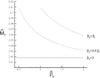 |
Fig. 3 Same as in Fig. 1, for n = 3. |
| In the text | |
 |
Fig. 4 Same as in Fig. 1, for n = 3/2. |
| In the text | |
Current usage metrics show cumulative count of Article Views (full-text article views including HTML views, PDF and ePub downloads, according to the available data) and Abstracts Views on Vision4Press platform.
Data correspond to usage on the plateform after 2015. The current usage metrics is available 48-96 hours after online publication and is updated daily on week days.
Initial download of the metrics may take a while.