| Issue |
A&A
Volume 540, April 2012
|
|
|---|---|---|
| Article Number | A92 | |
| Number of page(s) | 11 | |
| Section | Astronomical instrumentation | |
| DOI | https://doi.org/10.1051/0004-6361/201118568 | |
| Published online | 03 April 2012 | |
Spherical 3D isotropic wavelets
1 Laboratoire AIM, UMR CEA-CNRS-Paris 7, Irfu, SEDI-SAP, Service d’Astrophysique, CEA Saclay, 91191 Gif-sur-Yvette Cedex, France
e-mail: jstarck@cea.fr
2 Laboratoire d’Astrophysique, École Polytechnique Fédérale de Lausanne (EPFL), Observatoire de Sauverny, 1290 Versoix, Switzerland
Received: 2 December 2011
Accepted: 20 January 2012
Context. Future cosmological surveys will provide 3D large scale structure maps with large sky coverage, for which a 3D spherical Fourier-Bessel (SFB) analysis in spherical coordinates is natural. Wavelets are particularly well-suited to the analysis and denoising of cosmological data, but a spherical 3D isotropic wavelet transform does not currently exist to analyse spherical 3D data.
Aims. The aim of this paper is to present a new formalism for a spherical 3D isotropic wavelet, i.e. one based on the SFB decomposition of a 3D field and accompany the formalism with a public code to perform wavelet transforms.
Methods. We describe a new 3D isotropic spherical wavelet decomposition based on the undecimated wavelet transform (UWT) described in Starck et al. (2006). We also present a new fast discrete spherical Fourier-Bessel transform (DSFBT) based on both a discrete Bessel transform and the HEALPIX angular pixelisation scheme. We test the 3D wavelet transform and as a toy-application, apply a denoising algorithm in wavelet space to the Virgo large box cosmological simulations and find we can successfully remove noise without much loss to the large scale structure.
Results. We have described a new spherical 3D isotropic wavelet transform, ideally suited to analyse and denoise future 3D spherical cosmological surveys, which uses a novel DSFBT. We illustrate its potential use for denoising using a toy model. All the algorithms presented in this paper are available for download as a public code called MRS3D at http://jstarck.free.fr/mrs3d.html
Key words: large-scale structure of Universe / surveys / methods: analytical / methods: numerical / methods: statistical
© ESO, 2012
1. Introduction
Challenges in modern cosmology
The wealth of cosmological data in the last few decades (Larson et al. 2011; Schrabback et al. 2010; Percival et al. 2007b) has led to the establishment of a standard model of cosmology, which describes the Universe as composed today of approximately 4% baryons, 22% dark matter and 74% dark energy. The main challenges in modern cosmology are to understand the nature of both dark energy and dark matter, as well as the initial conditions of the Universe (Albrecht et al. 2006; Peacock et al. 2006). A thorough understanding of these three topics may lead to a revision of Einstein’s theory of General Relativity and our view of the early Universe.
New surveys are planned who aim to answer these important questions e.g. Planck for the CMB (Planck Collaboration 2011), DES (Dark Energy Survey, Annis et al. 2005), BOSS (Baryon Oscillation Spectroscopic Survey, Schlegel et al. 2007), LSST (Large Synoptic Survey Telescope, Tyson & LSST 2004) and Euclid (Laureijs et al. 2011) for weak lensing and the study of large scale structure with galaxy surveys.
The challenge with these upcoming large data-sets is to extract the cosmological information in the most suitable manner in order to test the cosmological paradigm. Depending on the signal one wishes to extract, and/or survey geometry, different bases may be more or less suitable (e.g., Fourier, spherical harmonic, configuration or wavelet space). Moreover, future surveys may be in 2D (e.g. Planck) or in 3D (e.g. galaxy or weak lensing surveys). Where 3D data is available, a tomographic analysis is possible (also known as 2D 1/2), or a full 3D analysis can be done. For data in spherical coordinates, this corresponds to a spherical Fourier-Bessel (SFB) decomposition (Heavens & Taylor 1995; Fisher et al. 1995; Castro et al. 2005; Erdoğdu et al. 2006a,b; Leistedt et al. 2012; Rassat & Refregier 2012).
Wavelet transform on the sphere
Wavelets are particularly well suited to the analysis of cosmological data (Martinez et al. 1993; Starck et al. 2006), since cosmological data can often be sparsely represented in wavelet space. 2D Wavelets have been used in many astrophysical studies (Starck & Murtagh 2006) for a broad range of applications such as denoising, deconvolution, detection, etc. CMB studies have motivated the development of 2D spherical wavelet decompositions. Continuous wavelet transforms on the sphere (Antoine 1999; Tenorio et al. 1999; Cayón et al. 2001; Holschneider 1996) have been proposed, mainly for non Gaussianity studies. In Starck et al. (2006), an invertible isotropic undecimated wavelet transform (UWT) on the sphere based on spherical harmonics was described, that can be also used for other applications such as deconvolution, component separation (Moudden et al. 2005; Bobin et al. 2008; Delabrouille et al. 2009), inpainting (Abrial et al. 2007, 2008), or Poisson denoising (Schmitt et al. 2010). A similar wavelet construction has been published in (Marinucci et al. 2008; Faÿ & Guilloux 2008; Faÿ et al. 2008) using so-called “needlet filters”, and in Wiaux et al. (2008), an algorithm was proposed which allows us to reconstruct an image from its steerable wavelet transform. Other multiscale transforms on the sphere such as ridgelets and curvelets have been developed (Starck et al. 2006), and are well adapted to detect anisotropic features. Other multiscale transforms on the sphere, such as ridgelets and curvelets, have been developed (Starck et al. 2006) and are well adapted to detect anisotropic features. An extension of this UWT has also been developed for polarised CMB data in Starck et al. (2009).
In this paper, we describe a new 3D isotropic spherical wavelet decomposition, which is reversible, and could therefore be useful for many different applications. It is based on the UWT proposed by Starck et al. (2006) and extended into 3D. The 3D-UWT proposed here can be used to analyse 3D data in spherical coordinates, such as a 3D galaxy or weak lensing survey with large (but not necessarily full) sky coverage.
2. Spherical 3D filtering using the spherical Fourier-Bessel transform
2.1. Spherical Fourier-Bessel transform
The SFB transform of a square integrable scalar field f(r,θ,φ) can be defined as: 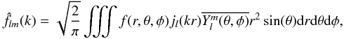 (1)where
  are spherical harmonics and jl are spherical Bessel functions and
  represents the complex conjugate of Y. Note Eq. (1) uses the same convention as Heavens & Taylor (1995) which differs slightly from that of Castro et al. (2005), Leistedt et al. (2012) and Rassat & Refregier (2012), as explained below. This expression allows the expansion of a 3D field provided in spherical coordinates onto a set of orthogonal functions:
  (2)From the orthogonality of the Ψlmk’s, the original field f(r,θ,φ) can be reconstructed from its SFB transform
  using the following inversion formula:
  (3)From this definition, the SFB transform can also be regarded as the commutative composition of two different transforms: a spherical harmonics transform (SHT) for the angular dimension and a spherical Bessel transform (SBT) for the radial dimension. In this work, the following convention is adopted to define the SHT of a function f(θ,φ) defined on the sphere:
  Our choice for Ψlmk allows us to give a symmetrical expression for the SBT and its inverse:
 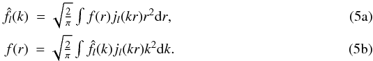 Although this symmetrical formulation for the SBT may differ from other works (e.g., Castro et al. 2005; Leistedt et al. 2012; Rassat & Refregier 2012), it will prove very convenient, especially to obtain a discretised transform (see Sect. 4).
2.2. Frequency filtering using the SFB transform
Spherical 3D filtering can be defined as the 3D convolution product of a 3D field in spherical coordinates with a 3D filter also provided in spherical coordinates. Using the relations presented in Sects. A.1 and A.2, it is possible to express such a product in terms of SFB coefficients and to relate those coefficients to regular Fourier coefficients.
To illustrate spherical 3D filtering on a simple case, let us consider a simple isotropic low-pass filter u whose 3D Fourier transform is U(k,θk,φk). The 3D Fourier transform of such a filter has a spherical symmetry and takes a simple form in spherical coordinates. Indeed, U(k,θk,φk) is a function only of k because of its symmetry, therefore U(k,θk,φk) = U(k). Furthermore, since U(k,θk,φk) is constant on every sphere centred on the origin in Fourier space, its SHT for a given k verifies ∀(l,m) ≠ (0,0), Ulm(k) = 0. As a result, the SFB transform of u has the following simple expression: 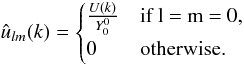 (6)Let us now consider a 3D field f defined in spherical coordinates. The filtered field v resulting from applying u to f is obtained using Eq. (A.8) simplified by the properties of g:
 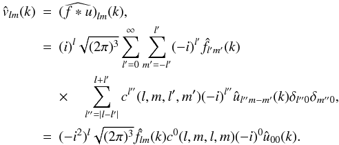 (7)Knowing that
  , the following expression is finally obtained:
  (8)In the special case of a 3D isotropic filter, frequency filtering is therefore easily obtained using the SFB transform and the filtered coefficients are simply the original coefficients multiplied by a function of k.
Although this filter seems overly simplistic, it will be shown in the following sections that such a low-pass filter is at the heart of the isotropic undecimated spherical 3D wavelet transform which makes direct use of Eq. (8).
3. Isotropic undecimated spherical 3D wavelet transform
An isotropic undecimated spherical wavelet transform defined on the sphere and based on the SHT was proposed in Starck et al. (2006). Now the aim is to transpose the ideas behind this transform to the case of data in 3D spherical coordinates. Indeed, the isotropic wavelet transform can be defined using only an isotropic low-pass filter. In the last section the necessary relations to apply such a filter have been obtained and the Isotropic Undecimated Spherical 3D Wavelet transform can now be defined.
3.1. Wavelet decomposition
Using the formalism introduced in the previous section, a Wavelet transform can be defined with the SFB transform. This isotropic transform is based on a scaling function φkc(r,θr,φr) with cut-off frequency kc and spherical symmetry. The symmetry of this function is preserved in the Fourier space and therefore, its SFB transform verifies  whenever (l,m) ≠ (0,0). Furthermore, due to its cut-off frequency, the scaling function verifies
  for all k ≥ kc. In other terms, the scaling function verifies:
 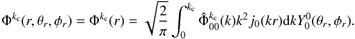 (9)Using relation (8) the convolution of the original data f(r,θ,φ) with Φkc becomes very simple:
 ![\begin{equation} \hat{c}^0_{l m}(k) = \widehat{\left[\Phi_{k_{\rm c}} \ast f\right]}_{l m}(k) = \sqrt{2} \pi \hat{\Phi}^{k_{\rm c}}_{0 0}(k) \hat{f}_{l m}(k). \end{equation}](/articles/aa/full_html/2012/04/aa18568-11/aa18568-11-eq37.png) (10)Using this scaling function, it is possible to define a sequence of smoother approximations cj(r,θr,φr) of a function f(r,θr,φr) on a dyadic resolution scale. Let Φ2 − jkc be a rescaled version of Φkc with cut-off frequency 2 − jkc. Then cj(r,θr,φr) is obtained by convolving f(r,θr,φr) with Φ2 − jkc:
(10)Using this scaling function, it is possible to define a sequence of smoother approximations cj(r,θr,φr) of a function f(r,θr,φr) on a dyadic resolution scale. Let Φ2 − jkc be a rescaled version of Φkc with cut-off frequency 2 − jkc. Then cj(r,θr,φr) is obtained by convolving f(r,θr,φr) with Φ2 − jkc: 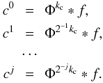 (11)Applying the SFB transform to the last relation yields:
 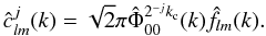 (12)This leads to the following recurrence formula:
 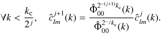 (13)Just like with the à trous algorithm by Starck et al. (2010), the wavelet coefficients { wj } can now be defined as the difference between two consecutive resolutions:
  (14)This choice for the wavelet coefficients is equivalent to the following definition for the wavelet function Ψkc:
 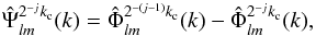 (15)so that:
 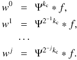 (16)By applying the SFB transform to the definition of the wavelet coefficients and using the recurrence formula verified by the cjs yields:
 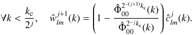 (17)Equations (17) et (13) which define the wavelet decomposition are in fact equivalent to convolving the resolution at a given scale j with a low-pass and a high-pass filter in order to obtain respectively the resolution and the wavelet coefficients at scale j + 1.
The low-pass filter, denoted here by hj, can be defined for each scale j by: 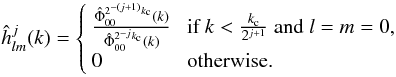 (18)Then the approximation at scale j + 1 is given by the convolution of scale j with hj:
 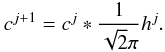 (19)In the same way, a high pass filter gj can be defined on each scale j by:
 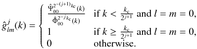 (20)Given the definition of Ψ, gj can also be expressed in the simple form:
 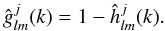 (21)The wavelet coefficients at scale j are obtained by convolving the resolution at scale j − 1 with gj − 1:
 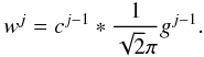 (22)In summary, the two relations necessary to recursively define the wavelet transform are:
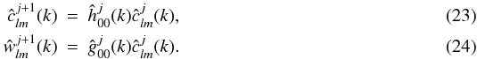
3.2. Reconstruction
Since the wavelet coefficients are defined as the difference between two resolutions, the reconstruction from the wavelet decomposition 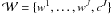 is straightforward and corresponds to the reconstruction formula of the à trous algorithm:
  (25)However, given the redundancy of the transform, the reconstruction is not unique. It is possible to take advantage of this redundancy to reconstruct cj from cj + 1 and wj + 1 by using a least squares estimate.
 |
Fig. 1 Scaling function and wavelet function for kc = 1. The y-axis represents the amplitude and the x-axis the frequency associated with the scaling function. The units of the amplitude must be those of the SFB transform. |
From the previous paragraph, the wavelet decomposition can be then recursively defined by:  If these relations are respectively multiplied by
  and
and  and then added together, the following expression is obtained for the least squares estimate of cj from cj + 1 and wj + 1:
  (28)where
  and
and  are defined as follows:
  Among the advantages of using this reconstruction formula instead of the raw sum over the wavelet coefficients is that there is no need to perform an inverse and then direct SFB transform to reconstruct the coefficients of the original data. Indeed, both the wavelet decomposition and reconstruction procedures only require access to SFB coefficients and there is no need to revert back to the direct space (although this will be required if one wishes to observe the power of each coefficient in real space as we do in Sect. 5 for denoising purposes).
3.3. Choice of a scaling function
Any function with spherical symmetry and a cut-off frequency kc would do as a scaling function but in this work we choose to use a B-spline function of order 3 to define our scaling function:  (31)where
  (32)The scaling function and its corresponding wavelet function are plotted in SFB space for different values of j in Fig. 1.
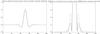 |
Fig. 2 Comparaison between spline and needlet wavelet functions on the sphere. The y-axis corresponds to amplitude and the x-axis to position. |
Other functions such as Meyer wavelets or the needlet function (Marinucci et al. 2008) can be used as well. Needlet wavelet functions have a much better frequency localisation than the wavelet function derived from the B3-spline but present more oscillations in the direct space. To illustrate this, we show in Fig. 2 two different wavelet functions. Figure 2 left shows 1D profile of the spline (continuous line) and the needlet wavelet function (dotted line) at a given scale. Figure 2 right shows the same function, but we have plotted the absolute value in order to better visualise their respective ringing. As it can be seen, for wavelet functions with the same main lob, the needlet wavelet oscillates much more than the spline wavelet. Hence, the best wavelet choice certainly depends on the desired applications. For statistical analysis, detection or restoration applications, we may prefer to use a wavelet which does not oscillate too much and with a smaller support, in this case the spline wavelet is clearly the correct choice. For spectral or bispectral analysis, where the frequency localisation is fundamental, then needlets should be preferred to the spline wavelet.
4. The discrete spherical Fourier-Bessel transform (DSFBT)
The spherical 3D wavelet formalism derived in the previous section is based on a continuous SFB transform. However, a continuous transform is not practical numerically and a discrete equivalent is required. In the case of galaxy surveys, where the underlying density field is sampled at discrete points, this problem can be addressed by combining a boundary condition with the discrete nature of the survey (see for e.g. Eqs. (5) and (7) in Leistedt et al. 2012, even though they use a slightly different SFB expansion as in this paper) which yields in this specific case a practical way to estimate discrete SFB coefficients. However this method cannot be used for the purpose of performing wavelet treatments since this requires a continuous field.
Indeed, to perform operations on the wavelet scales (e.g. for denoising purposes), one first needs to recover the wavelet coefficients in physical space, apply a treatment to those coefficients (e.g. thresholding) and then convert them back into SFB space (as required by the wavelet transform algorithm which operates in SFB space). This last operation requires a SFB transform which takes as input fields and not discrete galaxy surveys.
In this section, we show how a discretisation of the k spectrum in combination with a Healpix type angular pixelisation, can be used to build a fast Discrete SFB Transform (DSFBT) which allows for a novel and practical two-way conversion between the discrete SFB coefficients and discrete values of the field in physical space sampled on a spherical 3D grid.
4.1. The discrete spherical Bessel transform
The discretisation of the SFB transform along the radial component uses the well known orthogonality property of the spherical Bessel functions on the interval [0,R] . If f is a continuous function defined on [0,R] which verifies the boundary condition f(R) = 0 then the SBT defined by Eq. (5) can be expressed using SFB series: 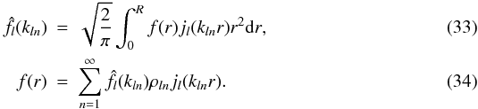 In this expression,
  where qln is the nth zero of the Bessel function of order l and the weights ρln are defined as:
  (35)Although this formulation provides a discretisation of the inverse SBT and of the k spectrum, the direct transform is still continuous and another discretisation step is required.
If a boundary condition of the same kind is applied to  so that
  , then by using the same result, the SFB expansion of is obtained by:
  where
where  and where the weights κln are defined as:
 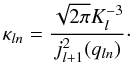 (37)The SBT being an involution,
  so that
  . Much like the previous set of equations had introduced a discrete kln grid, a discrete rln grid is obtained for the radial component. Since Eqs. (34) and (36b) can be used to compute f and
  for any value of r and k, they can in particular be used to compute f(rln) and
  where l′ does not have to match l. The SBT and its inverse can then be expressed only in terms of series:
 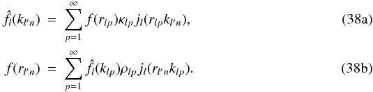 With these equations one can easily compute the SBT and its inverse without the need of evaluating any integral. Furthermore only discrete values of f and
  respectively sampled on rln and kln are required.
In practical applications, for a given value of l only a limited number Nmax of  and f(rln) coefficients can be stored so that rlNmax = R and klNmax = Kl. Since rln is defined by , for n = NmaxR and Kl are bound by the following relationship:
  (39)Therefore, from the value of R one can easily determine the appropriate value for Kl. Furthermore, because of the boundary conditions on and f, the series (38a) and (38b) can now be truncated to Nmax terms.
This truncation allows the use of a very convenient matrix formalism to represent the transform. In their explicit form, the two truncated sums can be rewritten as: 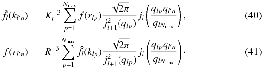 From these equations, a transform matrix Tll′ can be defined as:
 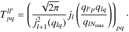 (42)This matrix allows the computation of on any grid kl′n from the values of f sampled on rln:
 ![\begin{equation} \left[\begin{matrix} \hat{f}_l(k_{l' 1}) \\ \hat{f}_l(k_{l' 2}) \\ \vdots \\ \hat{f}_l(k_{l' N_{\rm max}}) \end{matrix}\right] = \frac{1}{K_l^3} T^{l l'} \left[\begin{matrix} f(r_{l 1}) \\ f(r_{l 2}) \\ \vdots \\ f(r_{l N_{\rm max}}) \end{matrix}\right].\label{Direct_DSBT} \end{equation}](/articles/aa/full_html/2012/04/aa18568-11/aa18568-11-eq120.png) (43)Reciprocally, the inverse the values of f can be computed on any rl′n grid from sampled on kl′n using the exact same matrix:
(43)Reciprocally, the inverse the values of f can be computed on any rl′n grid from sampled on kl′n using the exact same matrix: ![\begin{equation} \left[\begin{matrix} f(r_{l' 1}) \\ f(r_{l' 2}) \\ \vdots \\ f(r_{l' N}) \end{matrix}\right] = \frac{1}{R^3} T^{l l'} \left[\begin{matrix} \hat{f}_l(k_{l 1}) \\ \hat{f}_l(k_{l 2}) \\ \vdots \\ \hat{f}_l(k_{l N}) \end{matrix}\right] .\label{Inverse_DSBT} \end{equation}](/articles/aa/full_html/2012/04/aa18568-11/aa18568-11-eq122.png) (44)The discrete SBT is defined by the set of Eqs. (43) and (44).
(44)The discrete SBT is defined by the set of Eqs. (43) and (44).
A simplified form of the transform could have been defined only for l = l′ so that Tll′ = Tl. However, keeping the distinction between the order of the transform l and the order of the grid on which the results are provided l′ will be crucial to the implementation of the DSFBT. Indeed, the order of the grid on which the function is sampled has to match the order of the transform but the resulting transform coefficients do not. Therefore, it will be possible to compute the result of the inverse SBT of any order l on a grid of order l0 so that only one radial grid of order l0 will be required. Nevertheless, for the direct transform, if the field is sampled on the radial grid of order l0, only the transform of order l0 can be computed. An additional result is required to be able to relate the SBT of different orders between them. This is achieved by combining relations (33) and (34):
![\begin{eqnarray} \hat{f}_l(k_{l n}) & = & \sqrt{\frac{2}{\pi}} \int_0^R \left[ \sum\limits_{m = 1}^{\infty} \hat{f}_{l_0}(k_{l_0 m}) \rho_{l_0 m} j_{l_0} (k_{l_0 m} r) \right] j_{l} ( k_{l n} r) r^2 {\rm d}r \nonumber ,\\ & = & \sqrt{\frac{2}{\pi}} \sum\limits_{m = 1}^{\infty} \hat{f}_{l_0}(k_{l_0 m}) \rho_{l_0 m} \int_0^R j_{l_0} (k_{l_0 m} r) j_{l} ( k_{l n} r) r^2 {\rm d}r \nonumber ,\\ & = & \sum\limits_{m = 1}^{\infty} \hat{f}_{l_0}(k_{l_0 m}) \frac{2}{ j_{l_0+1}^2(q_{l_0 m})} \int_0^1 j_{l_0} (q_{l_0 m} x) j_{l} ( q_{l n} x) x^2 {\rm d}x \nonumber ,\\ & = & \sum\limits_{m = 1}^{\infty} \hat{f}_{l_0}(k_{l_0 m}) \frac{2}{ j_{l_0+1}^2(q_{l_0 m})} W_{n m}^{l_0 l} ,\label{TransformConversion} \end{eqnarray}](/articles/aa/full_html/2012/04/aa18568-11/aa18568-11-eq126.png) (45)where the weights
(45)where the weights  are defined as:
  (46)The final expression in Eq. (45) is an important result which shows that the SBT of a given order can be expressed as the sum of the coefficients obtained for a different order of the transform, with the appropriate weighting. This means we can convert the Spherical Bessel coefficients of order l0 into coefficients of any other order l, which considerably speeds up calculations for the SBT. It is also worth noticing that the weights are simply geometric terms, i.e. independent of the field and can thus be tabulated.
We note that this approach is an extension of the discrete SBT presented in Lemoine (1994) using spherical Bessel functions and where the transform in Lemoine (1994) can be considered as a special case where l = l′.
4.2. A spherical 3D grid compatible with a discrete spherical Fourier-Bessel spectrum
As presented in Sect. 2.1, the SFB transform is the composition of a SHT for the angular component and a SBT for the radial component. Since these two transforms can commute, they can be treated independently and by combining discrete algorithms for both transforms, one can build a DSFBT. In this work, the angular part of the transform is implemented using the HEALPix pixelisation scheme while the radial component uses the discrete SBT algorithm presented in Sect. 4.1. The choice of these two algorithms introduces a discretisation of the SFB coefficients as well as a 3D gridding of the density in physical space.
The SFB coefficients are defined by Eq. (1) for continuous values of k. Assuming a boundary condition on the density field f, the discrete SBT can be used to discretise the values of k. The Discrete SFB coefficients are therefore defined as:  (47)for 0 ≤ l ≤ Lmax, − l ≤ m ≤ l and 1 ≤ n ≤ Nmax. These discrete coefficients are simply obtained by sampling the continuous coefficients on the kln grid introduced in the previous section.
To this discretised SFB spectrum corresponds a dual grid of the 3D space defined by combining the HEALPix pixelisation scheme and the discrete SBT.
Used for the computation of the SHT, the HEALPix scheme maps the sphere using curvilinear quadrilaterals of different shapes but equal area. Although other pixelisation schemes for the sphere such as IGLOO or GLESP could have been used, the choice of HEALPix is essentially motivated by the homogeneity of the pixelisation and by its comprehensive software package. For a given value of r, the field f(r,θ,φ) can therefore be sampled on a finite number of points using HEALPix.
The radial component of the transform is conveniently performed using the discrete SBT. Indeed, this algorithm introduces a radial grid compatible with the discretised kln spectrum. Although this radial grid rln depends on the order l of the SBT, it will be justified in the next section that only one grid rl0n is required to sample the field along the radial dimension. The value of l0 is set to 0 because in this case the properties of the zeros of the Bessel function ensure that r0n will be regularly spaced between 0 and R:  (48)For given values of θ and φ, the field f(r,θ,φ) can now be sampled on discrete values of r = r0n.
Combining angular and radial grids, the 3D spherical grid is defined as a set of Nmax HEALPix maps equally spaced between 0 and R. An illustration of this grid is provided in Fig. 3 where only one quarter of the space is represented for clarity.
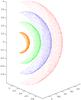 |
Fig. 3 Representation of the spherical 3D grid for the DSFBT (R = 1 and Nmax = 4) as described in Sect. 4 where the axes represent x,y,z and the grid points correspond to the centre of Healpix pixels and the radial grid is defined in Sect. 4.1. |
With this 3D grid, it will be possible to compute back and forth the SFB transform between a density field and its SFB coefficients. The details of the actual algorithm are provided in the next section.
4.3. Algorithm for the discrete spherical Fourier-Bessel transform (DSFBT)
Although the SHT and the SBT formally commute, some practical considerations on the order between the two operations are to be taken into account for their actual implementation. Here, a detailed algorithm of both the direct and inverse DSFBT is provided.
4.3.1. Direct transform
Given a density field f sampled on the spherical 3D grid, the SFB coefficients flmn are computed in three steps:
-
1)
For each n between 1 and Nmax the SHT of the HEALPix map of radius rl0n is computed. This yields flm(rl0n) coefficients.
-
2)
The next step is to compute the SBT of order l0 from the flm(rl0n) coefficients for every (l,m). This operation is a simple matrix product:
![\begin{equation} \left\lbrace\begin{matrix}\forall & 0 &\leq & l & \leq & L_{\rm max} \\ \forall & -l & \leq & m & \leq & l,\end{matrix} \right. \left[\begin{matrix} \hat{f}^{l_0}_{l m}(k_{l_0 1}) \\ \hat{f}^{l_0}_{l m}(k_{l_0 2}) \\ \vdots \\ \hat{f}^{l_0}_{l m}(k_{l_0 N_{\rm max}}) \end{matrix}\right] = \frac{T^{l_0 l_0}}{K^3} \left[\begin{matrix} f_{l m}(r_{l_0 1}) \\ f_{l m}(r_{l_0 2}) \\ \vdots \\ f_{l m}(r_{l_0 N_{\rm max}}) \end{matrix}\right]. \end{equation}](/articles/aa/full_html/2012/04/aa18568-11/aa18568-11-eq147.png) (49)This operation yields
(49)This operation yields  coefficients which are not yet SFB coefficients because the order of the SBT l0 does not match the order of the spherical harmonics coefficients l. An additional step is required.
 -
3)
The last step required to gain access to the SFB coefficients flmn is to convert the Spherical Bessel coefficients for order l0 to the correct order l that matches the spherical harmonics order. This is done by using relation (45):
 (50)where
  are defined by Eq. (46). This operation finally yields the
  coefficients.
4.3.2. Inverse transform
Let flmn be the coefficients of the SFB transform of the density field f, where the flmn coefficients can be calculated for a continuous density field using the direct transform described above or for a galaxy or halo catalogue using the public code 3DEX (Leistedt et al. 2012). Note that the 3DEX code can account for masked regions of missing data. The reconstruction of f on the spherical 3D grid requires two steps:
-
1)
First, from theflmn, the inverse discrete SBT is computed for all l and m. Again, this transform can be easily evaluated using a matrix product:
![\begin{equation} \left\lbrace\begin{matrix}\forall & 0 &\leq & l & \leq & L_{\rm max} \\ \forall & -l & \leq & m & \leq & l,\end{matrix} \right. \quad \left[\begin{matrix} f_{l m}(r_{l_0 1}) \\ f_{l m}(r_{l_0 2}) \\ \vdots \\ f_{l m}(r_{l_0 N_{\rm max}}) \end{matrix}\right] = \frac{T^{l l_0}}{R^3} \left[\begin{matrix} f_{l m 1} \\ f_{l m 2} \\ \vdots \\ f_{l m N_{\rm max}} \end{matrix}\right]. \end{equation}](/articles/aa/full_html/2012/04/aa18568-11/aa18568-11-eq153.png) (51)Here, it is worth noticing that the matrix Tll0 allows the evaluation of the SBT of order l and provides the results on the grid of order l0.
(51)Here, it is worth noticing that the matrix Tll0 allows the evaluation of the SBT of order l and provides the results on the grid of order l0. -
2)
From the spherical harmonics coefficients flm(rl0n) given at specific radial distances rl0n it is possible to compute the inverse SHT. For each n between 1 and Nmax the HEALPix inverse SHT is performed on the set of coefficients { flm(rl0n) } l,m. This yields Nmax HEALPix maps which constitute the sampling of the reconstructed density field on the 3D spherical grid.
5. Wavelet decomposition of a test density field
To illustrate the wavelet transform described in Sect. 3, a set of SFB Coefficients was extracted from a 3D density field using the DSFBT described in in Sect. 4. The test density field was provided by a cosmological N-body simulation which was carried out by the Virgo Supercomputing Consortium using computers based at Computing Centre of the Max-Planck Society in Garching and at the Edinburgh Parallel Computing Centre. We use their large box simulations1.
We first compute the SFB coefficients of the test density field by sampling the Virgo density field on the 3D grid illustrated in Fig. 3, for nside = 2048, lmax = 1023 and nmax = 512. In order to perform the SFB decomposition, we place ourselves in the middle of the box, and calculate the SFB coefficients out to r = 479/2 h-1 Mpc, setting the over-density field to zero outside of this spherical volume. In order to better visualise the data, we present in Fig. 4a the data in a cube spanning half the size of the original box (i.e. 239.5 h-1 Mpc), where the field has been reconstructed from the SFB coefficients, using the discrete inverse transform we discuss in Sect. 4.
From the SFB coefficients we calculate the wavelet decomposition, which yields the SFB coefficients of the various wavelet scales and the smoothed density field. Using the inverse DSFBT, the actual wavelet coefficients can be retrieved in the form of 3D density fields. These density fields corresponding to different wavelet scales are shown in Figs. 4b to e. The smoothed density field which arises from the wavelet decomposition is also shown in Fig. 4f, which is simply given by:  (52)
(52)
 |
Fig. 4 Spherical 3D wavelet decomposition of a density field for a box with side 239.5 h-1 Mpc. Panel a) shows the reconstructed density field directly using the initial SFB coefficients. Panels b–e) show the first four wavelet scales, while panel f) shows the smoothed density field. |
6. Application to wavelet hard thresholding (denoising)
In this section, a noise removal application based on wavelet thresholding is presented as an example of a potential use for the Isotropic Undecimated Spherical 3D Wavelet transform.
 |
Fig. 5 Wavelet Hard thresholding applied to a test density field. |
6.1. Thresholding
Many wavelet filtering methods have been proposed in the last twenty years. Hard thresholding consists of setting to 0 all wavelet coefficients which have an absolute value lower than a threshold Tj (non-significant wavelet coefficient):  where wj,k is a wavelet coefficient at scale j and at spatial position k.
Soft thresholding consists of replacing each wavelet coefficient by the value  where
where 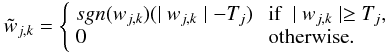 This operation is generally written as:
  (53)where (x) + = max(0,x).
In the case of Gaussian noise with a given standard deviation σ, a reasonable choice for the threshold Tj is Tj = Kσj, where j is the scale of the wavelet coefficient, σj is the noise standard deviation at the scale j, and K is a constant generally chosen between to 3 and 5. The standard deviation σj depends only on the chosen wavelet function and the noise level σ. More details can be found in Starck et al. (2010).
Other threshold methods have been proposed, like the universal threshold (Donoho & Johnstone 1994; Donoho 1993), or the SURE (Stein unbiased risk estimate) method (Coifman & Donoho 1995), but they generally do not yield as good results as the hard thresholding method based on the significant coefficients. Concerning the threshold level, the universal threshold corresponds to a minimum risk. The larger the number of pixels, the larger the risk is, and it is normal that the threshold T depends on the number of pixels ( , n being the number of pixels). The Kσ threshold corresponds to a false detection probability, the probability to detect a coefficient as significant when it is due to the noise. The 3σ value corresponds to 0.27% false detection.
6.2. Denoising experiment
We test the hard thresholding algorithm by using it to remove artificially added Gaussian noise on the Virgo density field (the simulation is described in Sect. 5). To conduct this experiment, the original density field taken from the n-body simulation has been used to compute an initial set of SFB coefficients (with lmax = 1023 and Nmax = 512) and out to r = 479 h-1 Mpc. Figure 5a shows a slice of the 3D density field reconstructed from these coefficients. A Gaussian noise was then added to the SFB coefficients, the reconstruction of this noisy density field is shown in Fig. 5b. The hard thresholding algorithm was subsequently applied to the noisy SFB coefficients using 5 wavelet scales. The resulting density field is reconstructed in Fig. 5c. The residuals are shown in Fig. 5d. The wavelet analysis means we can successfully remove the noise we artificially added on entry, without much loss to the large scale structure, though some of the smaller structures are removed.
7. Conclusion
Modern cosmology requires the analysis of 3D fields on large areas of the sky, i.e. where the field is best viewed in spherical coordinates. In this configuration, a spherical Fourier Bessel (SFB) transform is the most natural way to statistically analyse the field. Wavelet transforms have been shown to be ideally suited for cosmological fields, which tend to be sparse in wavelet space. The wavelet transform can be used e.g. for denoising, but there is yet no 3D wavelet transform in spherical coordinates.
We present in this paper a new 3D spherical wavelet transform, based on the undecimated wavelet transform (UWT) described in (Starck et al. 2006). In order to perform operations on the wavelet transforms (such as denoising), we require a discrete version of the SFB transform for both the direct and inverse transforms. We show a novel way to perform such a fast discrete spherical Fourier-Bessel transform (DSFBT) based on both a discrete Bessel transform and the HEALPIX angular pixelisation scheme.
Using the 3D wavelet transform and the DSFBT, both introduced in this paper, we denoise a test large scale structure data set, taken from the Virgo large box simulations2. We find we can satisfactorily remove artificially added Gaussian noise without much loss to the large scale structure. All the algorithms presented in this paper are available for download as a public code called MRS3D at http://jstarck.free.fr/mrs3d.html.
http://www.mpa-garching.mpg.de/Virgo/VLS.html, a ΛCDM simulation at z = 0, which was calculated using 5123 particles for the following cosmology: Ωm = 0.3,ΩΛ = 0.7,H0 = 70 km s-1 Mpc-1,σ8 = 0.9. The data cube provided is 479 h-1 Mpc in length.
Acknowledgments
The authors are grateful to Boris Leistedt, Pirin Erdoğdu, Ofer Lahav and Alexandre Réfrégier for useful discussions regarding the Spherical Fourier-Bessel decomposition and discretisation scheme. The 3D wavelet library uses Healpix software (Górski et al. 2002, 2005). This research is in part supported by the Swiss National Science Foundation (SNSF).
References
- Abrial, P., Moudden, Y., Starck, J., et al. 2007, J. Fourier Anal. Appl., 13, 729 [Google Scholar]
- Abrial, P., Moudden, Y., Starck, J., et al. 2008, Stat. Meth., 5, 289 [NASA ADS] [CrossRef] [Google Scholar]
- Albrecht, A., Bernstein, G., Cahn, R., et al. 2006 [arXiv:astro-ph/0609591] [Google Scholar]
- Annis, J., Bridle, S., Castander, F. J., et al. 2005 [arXiv:astro-ph/0510195] [Google Scholar]
- Antoine, J.-P. 1999, in Wavelets in Physics, ed. J. van den Berg (Cambridge University Press), 23 [Google Scholar]
- Baddour, N. 2010, J. Opt. Soc. Am. A, 27, 2144 [NASA ADS] [CrossRef] [Google Scholar]
- Bobin, J., Moudden, Y., Starck, J. L., Fadili, M., & Aghanim, N. 2008, Stat. Meth., 5, 307 [NASA ADS] [CrossRef] [Google Scholar]
- Castro, P. G., Heavens, A. F., & Kitching, T. D. 2005, Phys. Rev. D, 72, 023516 [NASA ADS] [CrossRef] [Google Scholar]
- Cayón, L., Sanz, J. L., Martínez-González, E., et al. 2001, MNRAS, 326, 1243 [NASA ADS] [CrossRef] [Google Scholar]
- Coifman, R., & Donoho, D. 1995, in Wavelets and Statistics, ed. A. Antoniadis, & G. Oppenheim (Springer-Verlag), 125 [Google Scholar]
- Delabrouille, J., Cardoso, J.-F., Le Jeune, M., et al. 2009, A&A, 493, 835 [NASA ADS] [CrossRef] [EDP Sciences] [Google Scholar]
- Donoho, D. 1993, in Proc. Symposia in Applied Mathematics, ed. A. M. Society, 47, 173 [Google Scholar]
- Donoho, D., & Johnstone, I. 1994, Biometrika, 81, 425 [CrossRef] [MathSciNet] [Google Scholar]
- Erdoğdu, P., Huchra, J. P., Lahav, O., et al. 2006a, MNRAS, 368, 1515 [Google Scholar]
- Erdoğdu, P., Lahav, O., Huchra, J. P., et al. 2006b, MNRAS, 373, 45 [NASA ADS] [CrossRef] [Google Scholar]
- Faÿ, G., & Guilloux, F. 2008 [arXiv:0807.2162] [Google Scholar]
- Faÿ, G., Guilloux, F., Betoule, M., et al. 2008, Phys. Rev. D, 78, 083013 [NASA ADS] [CrossRef] [Google Scholar]
- Fisher, K. B., Lahav, O., Hoffman, Y., Lynden-Bell, D., & Zaroubi, S. 1995, MNRAS, 272, 885 [NASA ADS] [Google Scholar]
- Górski, K. M., Banday, A. J., Hivon, E., & Wandelt, B. D. 2002, in Astronomical Data Analysis Software and Systems XI, ed. D. A. Bohlender, D. Durand, & T. H. Handley, ASP Conf. Ser., 281, 107 [Google Scholar]
- Górski, K. M., Hivon, E., Banday, A. J., et al. 2005, ApJ, 622, 759 [NASA ADS] [CrossRef] [Google Scholar]
- Heavens, A. F., & Taylor, A. N. 1995, MNRAS, 275, 483 [NASA ADS] [Google Scholar]
- Holschneider, M. 1996, J. Math. Phys., 37, 4156 [NASA ADS] [CrossRef] [Google Scholar]
- Larson, D., Dunkley, J., Hinshaw, G., et al. 2011, ApJS, 192, 16 [NASA ADS] [CrossRef] [Google Scholar]
- Laureijs, R., Amiaux, J., Arduini, S., et al. 2011 [arXiv:1110.3193] [Google Scholar]
- Leistedt, B., Rassat, A., Refregier, A., & Starck, J.-L. 2012, A&A, 540, A60 [NASA ADS] [CrossRef] [EDP Sciences] [Google Scholar]
- Lemoine, D. 1994, J. Chem. Phys., 101, 3936 [NASA ADS] [CrossRef] [Google Scholar]
- Marinucci, D., Pietrobon, D., Balbi, A., et al. 2008, MNRAS, 383, 539 [NASA ADS] [CrossRef] [Google Scholar]
- Martinez, V., Paredes, S., & Saar, E. 1993, MNRAS, 260, 365 [NASA ADS] [Google Scholar]
- Moudden, Y., Cardoso, J.-F., Starck, J.-L., & Delabrouille, J. 2005, EURASIP J. Appl. Signal Process., 15, 2437 [Google Scholar]
- Peacock, J. A., Schneider, P., Efstathiou, G., et al. 2006, ESA-ESO Working Group on Fundamental Cosmology, Tech. Rep. [Google Scholar]
- Percival, W. J., Cole, S., Eisenstein, D. J., et al. 2007b, MNRAS, 381, 1053 [NASA ADS] [CrossRef] [MathSciNet] [Google Scholar]
- Planck Collaboration 2011, A&A, 536, A1 [NASA ADS] [CrossRef] [EDP Sciences] [Google Scholar]
- Rassat, A., & Refregier, A. 2012, A&A, in press, DOI: 10.1051/0004-6361/201118638 [Google Scholar]
- Schlegel, D. J., Blanton, M., Eisenstein, D., & et al. 2007, in AAS Meeting Abstracts, 211, 132.29 [Google Scholar]
- Schmitt, J., Starck, J. L., Casandjian, J. M., Fadili, J., & Grenier, I. 2010, A&A, 517, A26 [NASA ADS] [CrossRef] [EDP Sciences] [Google Scholar]
- Schrabback, T., Hartlap, J., Joachimi, B., et al. 2010, A&A, 516, A63 [NASA ADS] [CrossRef] [EDP Sciences] [Google Scholar]
- Starck, J.-L., & Murtagh, F. 2006, Astronomical Image and Data Analysis (Springer), 2nd edn. [Google Scholar]
- Starck, J.-L., Moudden, Y., Abrial, P., & Nguyen, M. 2006, A&A, 446, 1191 [NASA ADS] [CrossRef] [EDP Sciences] [Google Scholar]
- Starck, J., Moudden, Y., & Bobin, J. 2009, A&A, 497, 931 [NASA ADS] [CrossRef] [EDP Sciences] [Google Scholar]
- Starck, J.-L., Murtagh, F., & Fadili, M. 2010, Sparse Image and Signal Processing (Cambridge University Press) [Google Scholar]
- Tenorio, L., Jaffe, A. H., Hanany, S., & Lineweaver, C. H. 1999, MNRAS, 310, 823 [NASA ADS] [CrossRef] [Google Scholar]
- Tyson, J. A., & LSST. 2004, in BAAS, 36, AAS Meeting Abstracts, 108.01 [Google Scholar]
- Wiaux, Y., McEwen, J. D., Vandergheynst, P., & Blanc, O. 2008, MNRAS 388, 770 [Google Scholar]
Appendix A: Spherical Fourier-Bessel transform and 3D convolution products
A.1. Spherical Fourier-Bessel transform and relation to the 3D Fourier transform
In order to have a better understanding of the SFB coefficients and of how to use them to perform filtering, the SFB transform can be related to the 3D Fourier transform. We follow a similar definition as the one presented in Baddour (2010), but using our conventions for the different transforms.The following convention will be used for the Fourier transform:  (A.1)where F denotes the Fourier transform of f. This formulation does not assume any coordinate system. However, to relate this transform to the SFB transform, it is possible to express this equation in spherical coordinates using the following expansion for the Fourier kernel:
  (A.2)where (k,θk,φk) and (r,θr,φr) are respectively the spherical coordinates of vectors k and r.
Substituting this expression for the kernel in the definition of the 3D Fourier transform yields: ![\appendix \setcounter{section}{1} \begin{eqnarray} F(k,\theta_k,\phi_k) & = & \frac{4\pi}{\sqrt{(2 \pi)^3}} \int_0^\infty \int_\Omega \sum_{l = 0}^{\infty} \sum_{m = -l}^{l} (-i)^l f(r, \theta_r, \phi_r) \nonumber \\ & & \times \quad j_l (k r) \overline{Y_l^m(\theta_r,\phi_r)} Y_l^m(\theta_k,\phi_k) {\rm d}\Omega r^2 {\rm d}r \nonumber ,\\ & = & \sum_{l = 0}^{\infty} \sum_{m = -l}^{l} (-i)^l \left[ \sqrt{\frac{2}{\pi}} \int_0^\infty \int_\Omega f(r, \theta_r, \phi_r) \right. \nonumber \\ & & \times \quad \left. j_l (k r) \overline{Y_l^m(\theta_r,\phi_r)} {\rm d}\Omega r^2 {\rm d}r \right] Y_l^m(\theta_k,\phi_k) \nonumber ,\\ & = & \sum_{l = 0}^{\infty} \sum_{m = -l}^{l} \left[ (-i)^l \hat{f}_{l m} (k) \right] Y_l^m(\theta_k,\phi_k) .\label{Relationship_Fourier_Bessel} \end{eqnarray}](/articles/aa/full_html/2012/04/aa18568-11/aa18568-11-eq190.png) (A.3)In the last equation, the expression of the Spherical Harmonics Expansion of F(k,θk,φk) for a given value of k can be recognised from Eq. (4b). In the Fourier space, the
(A.3)In the last equation, the expression of the Spherical Harmonics Expansion of F(k,θk,φk) for a given value of k can be recognised from Eq. (4b). In the Fourier space, the  are the spherical harmonics coefficients of F on a sphere of given radius k. In other words, the spherical harmonics coefficients Flm(k) of the 3D Fourier transform F(k,θk,φk) on a sphere of given radius k in Fourier space are the SFB coefficients for the same value k but multiplied by factor ( − i)l.
The relationship between 3D Fourier transform and SFB transform is therefore very simple. The SFB transform can be sought of as a mere Fourier transform in spherical coordinates. In the next sections, this relationship will be used to derive convolution and filtering relations for the SFB transform using the well known relations verified by the Fourier transform.
A.2. Expression of a 3D convolution product using the SFB transform
A prerequisite to the establishment of filtering relations is the expression of a 3D convolution product in terms of SFB coefficients. Let v(r,θr,φr) be the 3D convolution of f(r,θr,φr) and u(r,θr,φr). Then the 3D Fourier transform of v verifies:  (A.4)where ℱ denotes the 3D Fourier transform. From Eq. (A.3) the expression of the 3D Fourier transform in spherical coordinates is known in terms of SFB coefficients. Applying this relationship to V(k,θk,φk) in the last equation yields:
  (A.5)Then, by applying Eq. (A.3) to F and U one gets:
 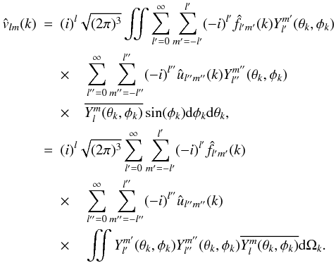 (A.6)The last integral over the two angular variables can be expressed as a Slater integral (which is a special case of the Gaunt integral) defined as:
 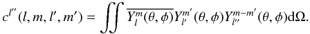 (A.7)The Slater integrals are only nonzero for | l − l′ | ≤ l′′ ≤ l + l′ which simplifies the expression of
  .
.
The SFB transform of the 3D convolution product is therefore: 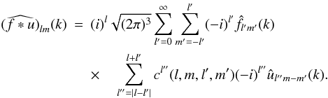 (A.8)
(A.8)
All Figures
|
Fig. 1 Scaling function and wavelet function for kc = 1. The y-axis represents the amplitude and the x-axis the frequency associated with the scaling function. The units of the amplitude must be those of the SFB transform. |
| In the text | |
|
Fig. 2 Comparaison between spline and needlet wavelet functions on the sphere. The y-axis corresponds to amplitude and the x-axis to position. |
| In the text | |
|
Fig. 3 Representation of the spherical 3D grid for the DSFBT (R = 1 and Nmax = 4) as described in Sect. 4 where the axes represent x,y,z and the grid points correspond to the centre of Healpix pixels and the radial grid is defined in Sect. 4.1. |
| In the text | |
|
Fig. 4 Spherical 3D wavelet decomposition of a density field for a box with side 239.5 h-1 Mpc. Panel a) shows the reconstructed density field directly using the initial SFB coefficients. Panels b–e) show the first four wavelet scales, while panel f) shows the smoothed density field. |
| In the text | |
|
Fig. 5 Wavelet Hard thresholding applied to a test density field. |
| In the text | |
Current usage metrics show cumulative count of Article Views (full-text article views including HTML views, PDF and ePub downloads, according to the available data) and Abstracts Views on Vision4Press platform.
Data correspond to usage on the plateform after 2015. The current usage metrics is available 48-96 hours after online publication and is updated daily on week days.
Initial download of the metrics may take a while.