| Issue |
A&A
Volume 540, April 2012
|
|
|---|---|---|
| Article Number | A11 | |
| Number of page(s) | 15 | |
| Section | Extragalactic astronomy | |
| DOI | https://doi.org/10.1051/0004-6361/201118357 | |
| Published online | 15 March 2012 | |
The ionized gas in the CALIFA early-type galaxies
I. Mapping two representative cases: NGC 6762 and NGC 5966⋆
1 Leibniz-Institut für Astrophysik Potsdam, innoFSPEC Potsdam, An der Sternwarte 16, 14482 Potsdam, Germany
2 Instituto de Astrofísica de Andalucía (CSIC), Apartado 3004, 18080 Granada, Spain
e-mail: This email address is being protected from spambots. You need JavaScript enabled to view it.
3 Centro de Astrofísica and Faculdade de Ciências, Rua das Estrelas 4150-762 Porto, Portugal
4 Centro Astronómico Hispano Alemán, Calar Alto (CSIC-MPG), C/ Jesús Durbán Remón 2, 04004 Almería, Spain
5 GEPI, Observatoire de Paris, UMR 8111, CNRS, Université Paris Diderot, 5 place Jules Janssen, 92190 Meudon, France
6 Departamento de Física-CFM, Universidade Federal de Santa Catarina, CP 476, 88040-900, Florianópolis, SC, Brazil
7 Sydney Institute for Astronomy, School of Physics, University of Sydney, NSW 2006, Australia
8 Astronomical Institute of the Ruhr-University Bochum, Universitaetsstr. 150, 44801 Bochum, Germany
9 Astrofísica de Canárias (IAC), vía Láctea s/n, 38200 La Laguna, Spain
10 Australian Astronomical Observatory, PO Box 296, Epping, Sydney NSW 1710, Australia
11 Department of Physics and Astronomy, Macquarie University, Sydney NSW 2109, Australia
12 Departamento de Astrofísica y CC. de la Atmósfera, Facultad de CC. Físicas, Universidad Complutense de Madrid, Avda. Complutense s/n, 28040 Madrid, Spain
13 Astronomisches Rechen Institut, Zentrum fuer Astronomie der Universitaet Heidelberg, Moenchhofstrasse 12–14, 69120 Heidelberg, Germany
14 Dep. Física Teórica y del Cosmos, Campus de Fuentenueva, Universidad de Granada, 18071 Granada, Spain
15 Departamento de Física Teórica, Universidad Autonoma de Madrid, Cantoblanco, 28049 Madrid, Spain
16 University of Vienna, Türkenschanzstrasse 17, 1180 Vienna, Austria
Received: 28 October 2011
Accepted: 23 December 2011
Abstract
As part of the ongoing CALIFA survey, we have conducted a thorough bidimensional analysis of the ionized gas in two E/S0 galaxies, NGC 6762 and NGC 5966, aiming to shed light on the nature of their warm ionized ISM. Specifically, we present optical (3745–7300 Å) integral field spectroscopy obtained with the PMAS/PPAK integral field spectrophotometer. Its wide field-of-view (1′ × 1′) covers the entire optical extent of each galaxy down to faint continuum surface brightnesses. To recover the nebular lines, we modeled and subtracted the underlying stellar continuum from the observed spectra using the STARLIGHT spectral synthesis code. The pure emission-line spectra were used to investigate the gas properties and determine the possible sources of ionization. We show the advantages of IFU data in interpreting the complex nature of the ionized gas in NGC 6762 and NGC 5966. In NGC 6762, the ionized gas and stellar emission display similar morphologies, while the emission line morphology is elongated in NGC 5966, spanning ~6 kpc, and is oriented roughly orthogonal to the major axis of the stellar continuum ellipsoid. Whereas gas and stars are kinematically aligned in NGC 6762, the gas is kinematically decoupled from the stars in NGC 5966. A decoupled rotating disk or an “ionization cone” are two possible interpretations of the elongated ionized gas structure in NGC 5966. The latter would be the first “ionization cone” of such a dimension detected within a weak emission-line galaxy. Both galaxies have weak emission-lines relative to the continuum[EW(Hα) ≲ 3 Å] and have very low excitation, log([Oiii]λ5007/Hβ) ≲ 0.5. Based on optical diagnostic ratios ([Oiii]λ5007/Hβ, [Nii]λ6584/Hα, [Sii]λ6717, 6731/Hα, [Oi]λ6300/Hα), both objects contain a LINER nucleus and an extended LINER-like gas emission. The emission line ratios do not vary significantly with radius or aperture, which indicates that the nebular properties are spatially homogeneous. The gas emission in NGC 6762 can be best explained by photoionization by pAGB stars without the need of invoking any other excitation mechanism. In the case of NGC 5966, the presence of a nuclear ionizing source seems to be required to shape the elongated gas emission feature in the “ionization cone” scenario, although ionization by pAGB stars cannot be ruled out. Further study of this object is needed to clarify the nature of its elongated gas structure.
Key words: galaxies: ISM / galaxies: elliptical and lenticular, cD / galaxies: individual: NGC 6762 / galaxies: individual: NGC 5966
Based on observations collected at the Centro Astronómico Hispano Alemán (CAHA) at Calar Alto, operated jointly by the Max-Planck-Institut für Astronomie and the Instituto de Astrofísica de Andalucía (CSIC).
© ESO, 2012
1. Introduction
Decades ago, early-type galaxies (ETGs) were thought to contain very little, if any, gas (e.g. Mathews & Baker 1971; Bregman 1978; White & Chevalier 1983). Subsequently, there have been many multiwavelength studies of ETGs that reveal a substantial multiphase interstellar medium (ISM; e.g. Trinchieri & di Serego Alighieri 1991; Goudfrooij et al. 1994; Macchetto et al. 1996; Caon et al. 2000; Kaviraj et al. 2011). The dominant component of their ISM is a hot (T ~ 106 − 107 K) gaseous component that emits in the X-rays (e.g. Forman et al. 1979; Fabbiano et al. 1992; O’Sullivan et al. 2001). Moreover, a warm (T ~ 104 K), less significant phase of the ISM has been generally detected with masses that are an order of magnitude lower than observed in spiral galaxies (Macchetto et al. 1996). The frequency of ETGs with a detectable warm ionized component in their ISM is significant, ranging from 60% to 80%, despite the differences in sample selection criteria and sample sizes. Narrowband Hα images of ETGs often reveal extended line emission, with radii of 5–10 kpc, which mostly have morphologies similar to the underlying stellar population (Demoulin-Ulrich et al. 1984; Kim 1989; Trinchieri & di Serego Alighieri 1991).
The nebular emission lines provide information about the physical properties and the ionization source(s) of the warm ISM. Understanding the sources required to ionize the gas is needed to investigate fundamental questions of the origin and the nature of the ionized gas in ETGs, which are still largely unsolved despite many studies. Most of the ETGs are optically classified as Seyfert nuclei or low-ionization nuclear emission-line regions (LINERs) based on their spectroscopic properties (see Annibali et al. 2010, and references therein). Several studies have discussed possible excitation mechanisms in ETGs, for example post-AGB (pAGB) stars, shocks, active galactic nuclei (AGNs), and OB stars (e.g. Binette et al. 1994; Stasińska et al. 2008; Sarzi et al. 2010; Annibali et al. 2010; Finkelman et al. 2010). Binette et al. (1994) claimed that white dwarfs and hot post-AGB stars provide sufficient ionizing photons to explain the observed generally low Hα equivalent widths (EW) and the LINER-like emission-line ratios observed in such galaxies (see also Sodré & Stasińska 1999; Stasińska et al. 2008). Sarzi et al. (2010) investigate the ionizing sources for the gas in ETGs based on SAURON integral-field spectroscopy (IFS) data whose spectra are limited to a relatively narrow wavelength range. The authors conclude that pAGB stars are the main source of ionizing photons in ETGs, and not fast shocks. In contrast, Annibali et al. (2010), by analyzing optical long-slit spectra of 65 ETGs, claim that their nuclear line-emission can be explained by excitation from the hard ionizing continuum from an AGN and/or fast shocks. However, they do not completely rule out a contribution from pAGB stars at large radii, even if their study of spatial variations in the warm ISM was limited by the area covered by their slits. Furthermore, it seems that ongoing star formation might be occurring in some ETGs, and the photoionization by hot young stars in some of these galaxies cannot be dismissed (e.g. Vílchez & Iglesias-Páramo 1998; Schawinski et al. 2007; Shapiro et al. 2010). This leaves us in the puzzling situation where all processes (photoionization from the old stellar population, young stellar population, and an AGN, or heating owing to fast shocks) may or may not all contribute to the excitation of the warm ionized medium in ETGs.
Basic data.
To address questions like “What are the sources of ionization that contribute to exciting line emission in ETGs?”, we initiated a program to analyze the warm ISM in ETGs within the context of the Calar Alto Legacy Integral Field Area (CALIFA) survey (Sánchez et al. 2012). CALIFA, through the use of wide-field, optical IFS, offers a unique observing capability to study the detailed properties of the extended optical emission-line gas in galaxies.
In this paper, we describe the results of a pilot study of two ETGs, NGC 6762 and NGC 5966. Our goal is to probe the properties of their warm ISM via spatially resolved emission-line diagnostics. These objects represent the two morphological types (S0 and E) among those ETGs first observed within CALIFA showing extended gas emission. As far as we know, this is the first investigation of the properties of the ionized gas in NGC 6762 and NGC 5966. The results for the remaining CALIFA ETGs hosting ionized gas will be presented in forthcoming papers.
The paper is organized as follows. In Sect. 2 we provide an overview of our two galaxies. Section 3 describes the observations and data reduction. The methodology used to subtract the stellar population from our spectra is presented in Sect. 4. In Sects. 5 and 6 we present a detailed analysis of the properties of the warm ionized medium in both galaxies. In Sect. 7 we discuss our results. Finally, in Sect. 8 we summarize our main conclusions from this study.
2. The sample: NGC 6762 and NGC 5966
Both NGC 6762 and NGC 5966 belong to the Uppsala General Catalogue (UGC) of Galaxies (Nilson 1973) and are among the most luminous objects (in z-band absolute magnitude, Mz) in the CALIFA survey sample (see Fig. 3 in Sánchez et al. 2012). The basic data of both galaxies are summarized in Table 1.
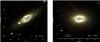 |
Fig. 1 Left panel: three-color, g, r, and i, composite SDSS image of NGC 6762. Foreground sources that have been disregarded in the subsequent spectral modeling and analysis are marked by crosses. Contours delineate an extremely faint spiral feature with a projected size of 31′′ × 9′′ disclosed by unsharp masking in the bulge of the galaxy. Right panel: SDSS color composite of NGC 5966 with contours from an unsharp masked image delineating a faint bar-like feature centered at the nucleus. North is up and east to the left in both images. |
In Fig. 1 we show three-color broad band image from the Sloan Digital Sky Survey (SDSS, York et al. 2000) of NGC 6762 (left panel) and NGC 5966 (right panel). For the lenticular galaxy NGC 6762, the SDSS images reveal a featureless disk-like morphology with no spiral arms, as expected from its morphological type. However, applying a flux-conserving unsharp masking technique (Papaderos et al. 1998) on the SDSS images reveals an extended (31″ × 9″) inclined spiral-like pattern that is traceable at extremely faint ( ≤ 1%) levels. Although not detected in the color maps owing to its extreme faintness, this feature indicates a complex formation history for the bulge component of NGC 6762 than what a cursory inspection of SDSS images may suggest. For this galaxy, we found overall red colors (g − i = 1.13 ± 0.03; g − r = 0.76 ± 0.04), characteristic of an old dominant stellar component (>6 Gyr) in both the disk and the bulge. In NGC 5966 (right panel of Fig. 1) unsharp masking reveals a compact bar-like structure 24′′ across centered on the compact nucleus. This structure has been associated with a radio source that is very likely powered by an AGN, instead of star formation, due to its low far-infrared flux upper limit (see Condon et al. 2002, and references therein). NGC 5966 shows approximately constant colors across its optical continuum emission with colors of g − i = 1.20 ± 0.02 and g − r = 0.80 ± 0.01. These red and uniform colors imply that NGC 5966 has an old dominant stellar population. As is the case for NGC 6762, no X-ray detection has been reported for NGC 5966.
3. Observations and data reduction
The observations of NGC 6762 and NGC 5966 were performed within the CALIFA survey, which aims to carry out a statistically complete IFS survey of over the full range of Hubble types present in the local universe (Sánchez et al. 2012). The survey is being conducted at the 3.5 m telescope of the Calar Alto observatory using the Potsdam MultiAperture Spectrograph (PMAS) in its PPAK mode (Roth et al. 2005; Kelz et al. 2006). A new CCD was installed in PMAS in 2009 (Roth et al. 2010) which is being used for the entire survey. Fibers in the PPAK bundle have a projected diameter on the sky of 2.7′′ and 331 out of 382 of the fibers form a hexagonal area covering a field of view of ~72′′ × 64′′ with a filling factor of ~65%. The remaining 51 fibers are dedicated to sky background (36 fibers) or used to obtain exposures of calibration lamps (15 fibers).
NGC 6762 and NGC 5966 were observed on 12 July 2010 and 1 April 2011, respectively, under photometric conditions and with a seeing of about 0 8-12. For this study, we used the V500 grating, which covers from 3745 to 7300 Å and has an effective spectral resolution of ~6.5 Å full width at half-maximum (FWHM) at ~5000 Å and a resolving power of R ~ 850. A dithering scheme with three pointings was used to sample the whole optical extent of each galaxy (see Sánchez et al. 2012, for details). Each pointing was observed for a total of 900 s, divided into three individual exposures to facilitate the removal of cosmic rays. The estimated limiting surface brightness in the V band for NGC 6762 and NGC 5966 are ~23.9 and 23.4 mag arcsec-2, respectively.
Data was reduced using the CALIFA pipeline (version 1.2). A detailed description of the steps followed during the reduction can be found in Sánchez et al. (2012) and the references therein. Briefly, first a master bias was created by averaging all the bias frames observed during the night and then subtracted from the science frames. Second, the location of the spectra in the CCD was determined using a continuum illuminated exposure taken before the science exposures. Then each spectrum was extracted from the science frames. Next, wavelength calibration and distortion correction were performed using arc lamps. Differences in the fiber-to-fiber transmission throughput were corrected by comparing the wavelength-calibrated extracted science frames with the corresponding continuum illuminated ones. The night-sky background spectrum, obtained by combining the spectra from the 36 dedicated sky fibers, is subtracted from the science-fiber spectra of the corresponding frame. Flux calibration was performed by comparing the extracted spectra of spectrophotometric standards stars from the Oke Catalogue (Oke 1990). The data were also corrected for the atmospheric extinction, using the airmass and the extinction of the observations as measured by the Calar Alto Extinction monitor. Both galaxies were observed with airmass <1.14. To construct the final data cube, all three pointings are combined. Using their relative positions and the PPAK position table, they are reformated into a single datacube with a spatial sampling of 1′′. Finally, the present version of the pipeline corrects for the effect of the Galactic extinction as reported by Schlegel et al. (1998): E(B − V) = 0.055 and 0.023 for NGC 6762 and NGC 5966, respectively.
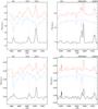 |
Fig. 2 NGC 6762: the panels to the left and right illustrate the main output from spectral synthesis in the blue and red spectral range, respectively, for a single spaxel in the brightest nuclear zone (top panels) and in the fainter periphery of the galaxy (~10′′ from the nucleus; bottom panels). The red and blue lines correspond to the observed and modeled stellar spectrum, respectively. By subtracting the latter from the former we obtain the pure nebular emission line spectrum (black). The spectra are offset in arbitrary units (au) for the sake of clarity. |
4. 2D modeling of the underlying stellar population
The emission lines in ETGs are generally extremely faint and often have EWs that are less than a few Å. This is a particular problem for the Balmer lines since the underlying absorption features from the stellar population can have EWs of the same order or more (e.g. Annibali et al. 2010). Determining emission-line intensities and intensity ratios is therefore a challenging task. To measure precisely emission-line fluxes and EWs, it is critical to model and remove the underlying stellar continuum that dilutes emission-line features. For this purpose, we used the STARLIGHT1 spectral synthesis code (Cid Fernandes et al. 2004) to model the stellar spectral energy distribution (SED) at each spaxel of the PPAK data cube.
The best-fitting stellar SED was then subtracted from the observed spectrum in order to isolate the pure emission line spectrum, which was then used to study the nebular component in ETGs. This way, in many cases, even weak emission lines (such as, e.g. the [Oi]λ6300 line) that seem to be absent in the observed spectra could be detected and measured accurately enough to yield astrophysically constraining results on the sources ionizing the gas. STARLIGHT uses various techniques for combining synthetic stellar populations to compute the best-fitting stellar SED. The best-fitting linear combination of N⋆ single stellar populations (SSPs), is obtained by using a nonuniform sampling of the parameter space based on the Markov Chain Monte Carlo algorithm, plus an approach called simulated annealing, and a convergence criterion similar to that proposed by Gelman & Rubin (1992), to approximately determine a global χ2 minimum.
We chose for our analysis SSPs from Bruzual & Charlot (2003, hereafter, BC03), which are based on the Padova 2000 evolutionary tracks (Girardi et al. 2000) and the Salpeter initial mass function (IMF) between 0.1 and 100 M⊙. The SSP library used here consists of three metallicities (0.5, 1 and 1.5 Z⊙) for 34 ages between 5 Myr and 13.6 Gyr. The intrinsic extinction was modeled as an uniform dust screen, adopting the extinction law by Cardelli et al. (1989). Line broadening effects, due to line-of-sight stellar motions, are accounted for in STARLIGHT by a convoluted Gaussian function.
The spectral synthesis models were computed spaxel by spaxel in an automatic manner using a pipeline written in the MIDAS2 script language and in Fortran, with additional modules that make use of PGplot and CFITSIO routines. Prior to fitting, the spectrum at each spaxel of the binned data cube was extracted, shifted to the rest frame, and resampled to a 1 Å resolution. Emission lines and spurious spectral features were flagged using either a predefined spectral mask or, additionally, a 3σ clipping routine applied on the net emission line component of each spectrum, after a coarse prefitting with a reduced SSP library. Spectral fits were carried out in the spectral region between 4000 Å and 6900 Å, because the signal-to-noise (S/N) bluewards of 4000 Å is generally too low for a reliable modeling of the stellar component. We disregarded the red end of the spectra (6900–7300 Å) because of its generally lower S/N, as well as spectral artifacts induced by vignetting in the outer zones of the PPAK FOV (see Sánchez et al. 2012)
The output from the pipeline was then put into data cubes of dimension 80 × 75 × 2800 where each spaxel contains the post-processed observed spectrum (3Dobs), best-fitting stellar SED (3Dmod), and pure emission line spectrum (3Dneb). Additionally, the pipeline stores in a fourth data cube (3Dres) the spatially resolved distribution of various relevant quantities returned by STARLIGHT or computed subsequently from its output. These include, among others, the reduced χ2 and the absolute deviation (ADEV) between the input spectrum and its best-fitting SED, the derived V band extinction (AV) for the stellar component, the stellar velocity, the luminosity-weighted and mass-weighted stellar age and metallicity, and the surface density, as well as mass and luminosity fraction of stellar population older than 108 yr. Illustrative examples of the observed, modeled, and emission-line spectrum for single spaxels in central and peripheral zones of NGC 6762 and NGC 5966 are displayed in Figs. 2 and 3.
As an approximate check of systematic uncertainties in the derived emission line fluxes (Sect. 3), we additionally ran STARLIGHT models based on MILES SSPs (Sánchez-Blázquez et al. 2006; Vazdekis et al. 2010) for similar range of stellar population parameters. We find that the typical variation of emission line fluxes for the two analyses is lower than 10%, or about the same order of magnitude as those due to uncertainties in emission line measurements themselves.
5. A 2D view of the warm ISM
5.1. Line fitting and map creation
After subtracting the underlying stellar population from the data cubes, we performed a Gaussian fit to the emission lines using the IDL-based routine mpfitexpr (Markwardt 2009) and derived the quantities of interest for each individual spaxel following the methodology described in Monreal-Ibero et al. (2011) and references therein. Then, we used these with the position of the spaxels within the data cube to create an image suitable to manipulation with standard astronomical software.
Line fitting in these galaxies is challenging since emission lines are very weak even after stellar continuum subtraction. Therefore, the solutions in velocity for Hα, and [Nii]λ6584 were used as initial guesses for the other remaining significant emission lines in order to guarantee robust flux estimates. In the emission-line maps presented in the following section, we show only the line fluxes with relative error <0.10 and spaxels with ADEV < 4%. This empirical threshold was found to provide a reasonable compromise between the galaxy area studied and the goodness of the fits to individual spaxels. Furthermore, such a conservative cut-off ensures that Balmer absorption features are adequately reproduced by synthetic stellar SEDs. The chosen ADEV cutoff selects spaxels within approximately the 22 and 22.5 g mag/◻″ isophote for NGC 6762 and NGC 5966, respectively, or equivalently the inner 8 and 13 zones of the respective plots in Fig. A.1. These isophotal levels correspond to photometric radii of ~1.5 reff for NGC 6762 and ~1.7 reff for NGC 5966, and thus the area studied contains most of the galaxy’s optical luminosity for both galaxies.
5.2. Continuum and emission line intensity maps
We constructed continuum and flux maps of the relevant emission lines in NGC 6762 and NGC 5966 (Figs. 4 and 5). Not all emission-line maps display the same area. The Hα and [Nii]λ6584 maps show a larger area than the [Oi]λ6300 maps, for example, because those lines are the brightest optical emission lines in our data sets. It is important to note that the quality criteria outlined in Sect. 5.1 are relatively conservative. There are regions of emission at greater distances from the nucleus than what is shown in Figs. 4 and 5, particularly in Hα, [Nii]λ6584, and [Sii]λλ6717, 6731. However, in such regions, the residuals due to the subtraction of the continuum are about the same order as the flux of the lines, so the line flux estimates are unreliable.
Figures 4 and 5 also present the distribution of the Hα equivalent width, EW(Hα), defined as the ratio between the Hα line flux and the neighboring, line-free continuum flux (~6390–6490 Å). This was measured in the observed spectra. The values of EW(Hα) are very low ( ≤ 3 Å) in comparison to values measured in star-forming galaxies, indicating that the stellar continuum dominates the overall emission in our galaxies. Our EW(Hα) measurements are within the range of values derived by Annibali et al. (2010) for their sample of ETGs.
The emission line morphology of NGC 6762 is disk-like and similar to the continuum emission. However, this is not the case for NGC 5966. The emission line maps of NGC 5966 show an elongated structure (along an axis at PA ~ 30°) extending out to at least 10′′ (~3 kpc) on either side of the nucleus, while the stellar continuum map displays an elliptical shape. The difference or similarity of the line and continuum emission is interesting and provides important clues to the nature of the gas that we discuss in Sect. 7.
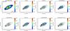 |
Fig. 4 Maps of the emission from NGC 6762. Upper row from left to right: the stellar component distribution as traced by a continuum map made from the median flux between 6390–6490 Å, a spectral region free of line emission (“pure continuum”); the EW(Hα); Hβ; [Oiii]λ5007. Bottom row from left to right: [Oi]λ6300; Hα; [Nii]λ6584; [Sii]λ6717, 6731. All maps are presented in logarithmic scale to emphasize the relevant morphological features. Flux units are 10-16 erg cm-2 s-1. The axis origin (i.e. the center of the PPak bundle) is marked with a cross. Contours corresponding to the stellar continuum map are overplotted on all maps for reference. The contour corresponding to the minimun level is − 1.70 dex and the interval between contours is 0.25 dex. North is up and east to the left. The pixel size is 1″ (~217 pc at our assumed distance to NGC 6762 of 45 Mpc). A bar showing the physical scale of 5 kpc is plotted at the lower righthand corner in the continuum map. |
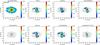 |
Fig. 5 Maps of the emission from NGC 5966. The panels show the same maps as outlined in Fig. 4. See the caption to that figure for details. The pixel size (1″) corresponds to ~334 pc at our assumed distance to NGC 5966 of 69 Mpc. |
5.3. The physical conditions in the warm ISM
The integral field spectra allow us to spatially probe the relative role of the various sources of ionization that could be responsible for the nebular emission observed in ETGs. In this section we present the radial and 2D spatial distribution of diagnostic emission-line ratios used to distinguish between different excitation mechanisms, and compare our measurements with those predicted by ionization models available in the literature.
5.3.1. Spatial distribution of diagnostic line ratios
The [Oiii]λ5007/Hβ, [Nii]λ6584/Hα, [Sii]λλ6717, 6731/Hα, and [Oi]λ6300/Hα line ratio maps for NGC 6762 and NGC 5966 are displayed in Fig. 6. For each galaxy, all the excitation maps display similar morphology, with relatively small spaxel-to-spaxel variations.
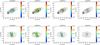 |
Fig. 6 Emission line ratio maps for NGC 6762 (top row) and NGC 5966 (bottom row). All maps are in logarithmic scale. The label at the top of each map indicates what emission line ratios are being displayed. The contours, linear scale, and orientation are the same as in Figs. 4 and 5. |
The radial profiles of the diagnostic line ratios provide constraints on the nature of the warm ionized medium in ETGs. We calculated the values of [Oiii]λ5007/Hβ and [Nii]λ6584/Hα within different annuli (computed as described in Appendix A) and plotted them as a function of the photometric radius R ⋆ , for both galaxies (Fig. 7). Emission-line fluxes are measured in the integrated pure emission line spectrum in each annulus using the IRAF3 task splot. The derived line fluxes were computed by fitting a Gaussian to each line. The line-flux errors are calculated using the expression by Castellanos et al. (2002), 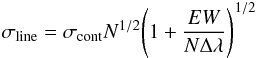 (1)where σcont is the standard deviation of the continuum near the emission line, N the width of the region used to measure the lines in pixels, Δλ the spectral dispersion in Å pix-1, and EW represents the EW of the line in Å. The EW values are obtained from the ratio between the line flux (measured in the pure emission line spectra) and the corresponding adjacent continuum flux (measured in the observed spectra). Since we are dealing with very faint emission with EW values < 3 Å (EW/NΔλ ≪ 1; see Figs. 10 and 11), we can neglect the addendum that involves the EW in the equation above.
Figure 7 shows that no significant radial trend is apparent in both [Oiii]λ5007/Hβ and [Nii]λ6584/Hα, well outside the nucleus with merely a weak tendency for decreasing values in NGC 6762. This suggests that there is no significant variation in nebular properties within the two objects and that the dominant ionization source is not confined to the nucleus since a decrease in excitation is expected for central source photoionization (e.g. Robinson et al. 1994; Whittle et al. 2005).
The majority of the spaxels in the cubes of NGC 6762 and NGC 5966 are characterized by log([Oiii]λ5007/Hβ) ≤ 0.5, indicating relatively low excitation (Figs. 6 and 7). Sarzi et al. (2010) find that 75% of their sample of ETGs show log([Oiii]λ5007/Hβ) in the range 0.0–0.5. High values of [Nii]λ6584/Hα, [Sii]λλ6717, 6731/Hα, and [Oi]λ6300/Hα are found in both galaxies, unlike in star-forming galaxies (e.g. Alonso-Herrero et al. 2010). In our galaxies, generally [Nii]λ6584 is brighter than Hα ([Nii]λ6584/Hα > 1.00 for most of spaxels), and [Oi]λ6300/Hα can be as high as ~0.40.
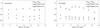 |
Fig. 7 Radial distribution of the [Oiii]λ5007/Hβ (triangle), [Nii]λ6584/Hα (square), and Hβpred./Hβobs. (cross; this ratio is discussed in Sect. 7) for NGC 6762 (left panel) and NGC 5966 (right panel). |
5.3.2. Diagnostic diagrams
The standard diagnostic diagrams (Baldwin et al. 1981, hereafter BPT) are widely used to probe the dominant ionizing source in galaxies (e.g. Kewley et al. 2006; Kehrig et al. 2008; Monreal-Ibero et al. 2010). The BPT diagrams, on a spaxel-by-spaxel basis, for NGC 6762 and NGC 5966 are shown in Figs. 8 and 9, respectively: [Oiii]λ5007/Hβ vs. [Nii]λ6584/Hα (left panels), [Oiii]λ5007/Hβ vs. [Sii]λλ6717, 6731/Hα (middle panels), and [Oiii]λ5007/Hβ vs. [Oi]λ6300/Hα (right panels). The line ratios are not corrected for reddening, but their reddening dependence is negligible since they are calculated from lines which are close to each other in wavelength space. As a guide to the reader, the data points with highest F(Hα) (i.e. 0.20 ≲ F(Hα)/F(Hα)peak ≲ 1.00; the high surface brightness zone) are the closest to the nucleus, within a circular area with radius ~4′′ (bottom rows of Figs. 8 and 9). The spaxels covering the more external regions of each galaxy (where F(Hα)/F(Hα)peak ≤ 0.20) are shown in the top rows of Figs. 8 and 9. For the galaxy NGC 5966, the [Oi]λ6300/Hα diagram is presented only for its inner region owing to the faintness of the [Oi]λ6300 emission (Fig. 9). According to the spectral classification scheme indicated in each figure, our emission line ratios in the diagnostic diagrams for most positions in both galaxies fall in the general locus of LINER-like objects. The relative uncertainty of our line-ratio measurements plotted in Figs. 8 and 9 is typically ≲ 15%. An analysis of the ionized gas in the central region of NGC 6762 suggests that it is dominated by a ionization source other than star formation (Sánchez et al. 2012).
Three grids of ionization models are overplotted on the BPT diagrams (Figs. 8 and 9). The plotted AGN models have an electron density, ne = 100 cm-3, metallicities of solar (Z = Z⊙) and twice solar, a range of ionization parameter (−3.6 < logU < 0.0) and a power-law ionizing spectrum with spectral index α = −1.4. While the AGN photoionization models of Groves et al. (2004) are consistent with most of the spaxels in the [Nii]λ6584/Hα diagrams for NGC 5966, this is not the case of NGC 6762 where the measurements of [Nii]λ6584/Hα in the brightest area are not reproduced well by the AGN grids (bottom-left panel of Fig. 8). In the [Sii]λλ6717, 6731 diagram the data are merely fit by the AGN models in NGC 6762, and no match between observations and models is seen for NGC 5966. The measurements of [Oi]λ6300/Hα are not reproduced by these models for either of the two galaxies. A harder ionizing continuum, with α = −1.2, will boost [Sii]λλ6717, 6731 and [Oi]λ6300 relative to Hα, yielding a better fit in the [Oi]λ6300/Hα BPT diagram, while providing a poorer match with the [Sii]λλ6717, 6731/Hα measurements.
We also compared our results with shock models (Allen et al. 2008). In Figs. 8 and 9, we plot the grids with Z = Z⊙, preshock densities between 0.1 cm-3 and 100 cm-3, shock velocities from 100 to 1000 km s-1, and preshock magnetic field B = 1 μG. Shock models with a range of magnetic field strengths (e.g. B = 5, 10 μG) match our observations. Interstellar magnetic fields of B ~ 1−10 μG are typical of what is observed in elliptical galaxies (e.g. Mathews & Brighenti 1997). The low ne of these models are consistent with the values derived here (Tables 2 and 3). Overall, shock models reproduce the majority of our data in the three emission-line ratio diagrams. The shock grids with lower metallicity (e.g. LMC and SMC metallicities) are not consistent with our measurements.
Furthermore, we compare our observations to the photoionization models for pAGB stars with Z = Z⊙ (Binette et al. 1994). These models are consistent with most of our observations, except for the highest values of [Nii]λ6584/Hα [log([Nii]λ6584/Hα) > 0.1]. The model with Z = 1/3 Z⊙ is shifted towards lower values on the x-axis of the three BPTs, and it gives a much poorer match to the measurements in the [Nii]λ6584/Hα diagram. The pAGB scenario has recently been revisited by Stasińska et al. (2008), whose extensive grid of photoionization models (see their Fig. 5) cover most of the regions occupied by our spatially resolved measurements.
Since all of our emission line ratios appear to fall in the LINER region of the BPT diagrams (Figs. 8 and 9), we also put our spatially resolved line measurements in the WHAN diagram (EW(Hα) vs. log([Nii]λ6584/Hα); Figs. 10 and 11) introduced by Cid Fernandes et al. (2010). The authors argue that such a diagram is useful in distinguishing between two different types of objects that may lead to emission line ratios like those observed in LINERs and similar to what we observe in NGC 6762 and NGC 5966. In the WHAN diagram, galaxies with LINER (-like) emission are thus classified either as objects that present a weak AGN or the so-called retired galaxies (RG), objects that are not forming stars anymore and are ionized by their pAGB stars. Just as in the BPT diagrams, we split our data into two bins: the left and righthand panels of Figs. 10 and 11 show the spaxels for the outer (F(Hα)/F(Hα)peak ≤ 0.20) and inner (0.20 ≲ F(Hα)/F(Hα)peak ≲ 1.00) regions, respectively. The location of our data in this diagram are, for most emission line regions, compatible with the gas emission expected for photoionization by pAGB stars.
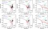 |
Fig. 8 Diagnostic diagrams for NGC 6762. From left to right: log ([Oiii]λ5007/Hβ) vs. log ([Nii]λ6584/Hα), log ([Oiii]λ5007/Hβ) vs. log ([Sii]λ6731,6717/Hα) and log ([Oiii]λ5007/Hβ) vs. log ([Oi]λ6300/Hα). The upper and bottom rows show the spaxels with F(Hα)/F(Hα)peak ≤ 0.20 and 0.20 ≲ F(Hα)/F(Hα)peak ≲ 1.00, respectively. The black solid curve (in all three panels) is the theoretical maximum starburst model from Kewley et al. (2001), devised to isolate objects whose emission line ratios can be accounted for by the photoionization by massive stars (below and to the left of the curve) from those where some other source of ionization is required. The black-dashed curves in the [Sii]λ6731,6717/Hα and [Oi]λ6300/Hα diagrams represent the Seyfert-LINER dividing line from Kewley et al. (2006) and transposed to the [Nii]λ6584/Hα by Schawinski et al. (2007). The predictions of different ionization models for ionizing the gas are overplotted in each diagram. The red lines represent the shock grids of Allen et al. (2008) with solar metallicity and preshock magnetic field B = 1.00 μG. For the grid of shock models, the solid lines show models with increasing shock velocity Vs = 100, 200, 300, 1000 km s-1, and dotted lines the grids with densities ne from 0.1 cm-3 to 100 cm-3. Grids of photoionization by an AGN (Groves et al. 2004) are indicated by green curves, with ne = 100 cm-3 and a power-law spectral index of − 1.4. The corresponding dashed-lines show models for Z = Z⊙ and Z = 2 Z⊙ (from left to right), and solid lines trace the ionization parameter log U, which increases with the [Oiii]λ5007/Hβ ratio from log U = −3.6, − 3.0, 0.0. We downloaded the shock and AGN grids from the web page http://www.strw.leidenuniv.nl/~brent/itera.html. The boxes show the predictions of photoionization models by pAGB stars for Z = Z⊙ and a burst age of 13 Gyr (Binette et al. 1994). |
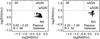 |
Fig. 10 EW(Hα) vs. log([Nii]λ6584/Hα) for NGC 6762. The left and right panels show the spaxels with F(Hα)/F(Hα)peak ≤ 0.20 and 0.20 ≲ F(Hα)/F(Hα)peak ≲ 1.00, respectively. SF = pure star-forming galaxies; sAGN = strong AGN; wAGN = weak AGN; RG = retired galaxies. The dividing lines are transpositions of the SF/AGN borders from Kewley et al. (2001, 2006) and Stasińska et al. (2006), and the Kewley et al. (2006) Seyfert/LINER division (see Cid Fernandes et al. 2010). |
5.4. Kinematics
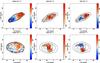 |
Fig. 12 Kinematics maps of NGC 6762 (top row) and NGC 5966 (bottom row): stellar velocity field (left panels), corrected velocity dispersion maps (middle panels) and radial velocity maps (right panels), as measured from Hα. The contours, orientation, and linear scale are the same as in Figs. 4 and 5. |
Figure 12 shows, for both galaxies, the stellar velocity field and the maps of corrected velocity dispersion, σ(Hα), and of radial velocity of the ionized gas, derived from the Hα emission line. The values of σ(Hα) are corrected for the instrumental profiles as measured from arc lines. The relative radial velocity of the Hα lines ranges from ~−130 km s-1 to ~180 km s-1 for NGC 6762, and from ~−100 km s-1 to ~ 160 km s-1 for NGC 5966. The typical uncertainty in the velocities are < 15 km s-1 (see Sánchez et al. 2012). The typical value of σ(Hα) is ~200 km s-1 in both NGC 6762 and NGC 5966. We estimated the errors for σ(Hα) based on a Monte Carlo simulation. The corresponding errors are ~10−20 km s-1 for NGC 6762 and 30−40 km s-1 for NGC 5966. For a sample of ~50 ETGs, Sarzi et al. (2006) find ionized gas velocities (estimated using the [Oiii]λ5007 line), between ~−250 km s-1 and ~250 km s-1 and gas velocity dispersions as high as 250 km s-1.
NGC 6762 displays an overall smooth rotation pattern along the SE-NW direction in both the gas and stellar velocity fields. NGC 5966 shows gas kinematics that are decoupled with respect to that of the stars. The orientation of the stellar component is roughly aligned SE to NW, with the stars in the NW part having a higher recessional velocity. The axis of the ionized gas in NGC 5966 is roughly orthogonal to that of the stars. Both cases, i.e. stars-ionized gas kinematically aligned and misaligned, have been observed in ETGs and help for determining the origin of the ionized gas in these galaxies (e.g. Davis et al. 2011, references therein). For instance, Sarzi et al. (2006) conclude that in half of their objects with gas kinematics decoupled from the stellar kinematics, this decoupling suggests an external origin for the gas. A deeper analysis of the complex kinematics in NGC 5966 is beyond the scope of this paper and will be presented elsewhere.
6. Spectral classification vs. aperture size
Observed emission line fluxes in units of 10-16 erg cm-2 s-1 and physical properties from different apertures for NGC 6762.
Observed emission line fluxes in units of 10-16 erg cm-2 s-1 and physical properties from different apertures for NGC 5966.
In this section we present the analysis of 1D spectra extracted within circular apertures of increasing diameter (5′′, 10′′ and 30′′) centered on the intensity maximum of the red stellar continuum. These apertures correspond to radii of 0.35, 0.7, and 2.1 reff for NGC 6762 and to 0.24, 0.47 and 1.4 reff for NGC 5966. We also extracted the integral spectrum by summing the emission from each spaxel within the [Nii]-Hα emitting area of each ETG, covering ~300 arcsec2 for both galaxies (~14 kpc2 ~ 5  and 33 kpc
 for NGC 6762 and NGC 5966, respectively). Two additional 1D spectra were extracted for NGC 5966, corresponding to the SW and NE regions of the elongated gas structure observed in the emission-line and velocity maps (Figs. 5 and 12). Emission-line fluxes were measured in the 1D spectra as described in Sect. 5.3.1 and given in Tables 2 and 3, together with the spectroscopic properties. Line fluxes quoted in the tables are not corrected for internal reddening.
We obtained the ne from the [Sii]λ6717/λ6731 line ratio using the IRAF nebular package (Shaw & Dufour 1995). The derived estimates for ne place all of the n-diameter aperture zones in the low-density regime of the [Sii] doublet (ne < 100 cm-3).
The logarithmic reddening, c(Hβ), was computed from the ratio of the measured-to-theoretical Hα/Hβ, assuming the Galactic reddening law of Cardelli et al. (1989) and an intrisic value of Hα/Hβ = 2.86 (Case B, electron temperature Te = 104 K, ne = 100 cm-3). At relatively low densities, the theoretical Hα/Hβ values vary from ~3.00 (Te = 5 × 10³ K) to ~2.75 (Te = 20 × 103 K). Since we are not able to estimate the Te of the warm ISM, we decided to adopt the intermediate value of 2.86 in this work. For some zones in NGC 5966, we adopt c(Hβ) = 0.0 since the corresponding Hα/Hβ values are consistent with no reddening within the errors. A different assumption from 2.86 would not change our results since most of quantities treated in this paper [e.g. [Oiii]λ5007/Hβ, [Nii]λ6584/Hα, EW(Hα)] slightly depend on reddening corrections.
From the integrated spectra (covering all of the Hα emitting region from each galaxy), we estimate the values of the reddening-corrected Hα luminosities, L(Hα): 6.0 ± 0.5 × 1039 erg s-1 (NGC 6762) and 5.8 ± 0.2 × 1039 erg s-1 (NGC 5966). These values are within the Hα luminosity range measured for luminous ETGs generally (Macchetto et al. 1996). For NGC 6762, we checked how much L(Hα) would change by adopting various values of Hα/Hβ (2.75 to 3.00), and found that the variations are within the quoted uncertainties.
Spectra constructed from apertures with a range of diameters allow us to evaluate how aperture effects may affect the spectral classification of the ETGs under study. The observed flux ratios ([Oiii]λ5007/Hβ, [Nii]λ6584/Hα, [Sii]λλ6717, 6731/Hα, and [Oi]λ6300/Hα), for both galaxies, are consistent with LINER-type emission based on the BPT diagrams (Figs. 8 and 9), independent of the aperture size (Tables 2 and 3). Splitting the elongated gas emission in NGC 5966 into two separate regions on either side of the nucleus suggests that both regions have the same spectral classification in the diagnostic BPT diagrams (Table 3). This indicates that the properties of the ionized gas do not vary significantly across the PPAK FOV for both galaxies. This is consistent with the results of an analysis of the radial profiles (Sect. 5.3.1). However, one should be cautious when interpreting the nebular spectra from integrated apertures. The presence of different ionization sources and the way they are spatially distributed might play roles in the spectral classification in the various apertures. For instance, from a sample of luminous infrared galaxies, Alonso-Herrero et al. (2009) find that the nuclear and integrated line-ratios give different spectral classifications in the BPT diagrams for some of their objects. In this case, this was interpreted as the result of an increased contribution of extra-nuclear high surface-brightness HII regions to the integrated emission of these galaxies.
7. Discussion
Based on our EW and diagnostic line ratios measurements, both NGC 6762 and NGC 5966 are weak emission-line galaxies in which most of spaxels can be classified as LINER-like (Figs. 8–11). Different ionizing mechanisms (e.g. pAGB stars, AGN, shocks, massive stars) have been proposed to explain LINER-like excitation in ETGs, but it is still a matter of debate (Sect. 1). In the previous sections we presented diagnostics that help distinguish between these different ionizing sources, including the overall morphology of the emission line gas. In the following we discuss which one(s) might be more likely to power the emission lines in these two galaxies based on our analysis.
According to the WHAN diagrams (Figs. 10 and 11), NGC 6762 and NGC 5966 are classified as RG, objects that have stopped forming stars and are ionized by the pAGB stars contained in them (Cid Fernandes et al. 2010). A central black hole may be present in RGs, but it is not expected to dominate the ionization budget (Cid Fernandes et al. 2011). Solar-metallicity photoionization models for pAGB stars are able to reproduce the majority of our spatially resolved data (Figs. 8 and 9; Binette et al. 1994), except for the high [Nii]λ6584/Hα ratios in the central region of NGC 6762, which are not reproduced even by a high metallicity model (Z = 3 Z⊙). However, one should bear in mind that in these photoionization models, the metallicity, Z, is a scaling factor of relative abundances of every element with respect to H, although it is known that the N/O ratio in galaxies is not (necessarily) constant (e.g. Mollá et al. 2006). The models by Stasińska et al. (2008), which are essentially updated versions of the Binette et al. (1994) ones, do not consider N/O to be a constant and do extend towards larger [Nii]λ6584/Hα. Photoionization models by pAGB stars are therefore consistent with the line ratios in both ETGs studied here.
To investigate whether pAGB stars can account for the ionizing flux in NGC 6762 and NGC 5966, we also computed the rate of the Lyman continuum photons expected from the surface density and age distribution of pAGB stars that we derived in each spaxel and used it to predict the Balmer emission fluxes, assuming case B, Te of 104 K and low densities (ne ≪ 104 cm-3). We also allow for calculating the Balmer emission line fluxes under the assumption that the warm ISM has the same foreground extinction as the stars. Since the stellar extinction derived is generally low (AV ≲ 0.3 mag), this assumption has only a minor influence on the final results. The predicted Balmer Hβ intensity was computed for different annuli (see the Appendix). In Fig. 7 we plot the Hβ predicted-to-observed flux ratio (Hβpred./Hβobs.) for both galaxies as a function of R ⋆ . Typical values of Hβpred./Hβobs. are close to 1 for NGC 6762, suggesting that pAGB stars can produce enough ionizing photons to explain the Balmer line fluxes. In the case of NGC 6762, the morphology of gas and stellar emission following each other is an additional and strong argument supporting the hypothesis that pAGB stars are responsible for ionizing the gas. In NGC 5966, the Hβpred./Hβobs. values are slightly greater than 1 on average for R ⋆ ≲ 8 arcsec, and decrease to < 1 for larger radii where the elongated gas emission dominates, indicating that another excitation source is likely needed. We discuss this further at the end of this section.
To probe the ionization by an AGN, we compare our observed line ratios ([Oiii]λ5007/Hβ, [Nii]λ6584/Hα, [Sii]λλ6717, 6731/Hα, [Oi]λ6300/Hα) with the AGN models of Groves et al. (2004). In Figs. 8 and 9 we represent the AGN-grids that better reproduce the majority of the spaxels in both galaxies (see Sect. 5.3.2 for details). However, for both galaxies, none of the AGN photoionization models are able to reproduce our spatially-resolved line ratios in all of the three BPT diagrams simultaneously. The relative radial constancy of the [Oiii]λ5007/Hβ and [Nii]λ6584/Hα ratios (Fig. 7) also argue against an AGN as the dominant ionization source in both NGC 6762 and NGC 5966 unless the ratio of ionizing photon intensity to the gas density is approximately constant.
Examples of extended LINER-like excitation from shocks can be found in the literature (e.g. Monreal-Ibero et al. 2006; Farage et al. 2010; Rich et al. 2011). Here, the detection of [Oi]λ6300 suggests the presence of shocks (e.g. Dopita 1976). To assess the role of excitation by shocks, the observations in the BPTs are compared to the fast shock models from Allen et al. (2008) (Figs. 8 and 9). A large fraction of the spaxels in both galaxies are reproduced by shock grids with velocities higher than ~200 km s-1. Outflows and accretion into a central black hole and collisions between gas clouds have been suggested as possible sources of mechanical energy that are able to account for such high velocity shocks (e.g. Dopita & Sutherland 1995; Dopita et al. 1997; Annibali et al. 2010, and references therein). From our data, the estimated average gas velocity dispersion σ, as measured from the Hα line, is ~200 km s-1 for both objects (Sect. 5.4), suggesting that fast shock-ionization cannot be ruled out in our galaxies. X-ray data would help in constraining the role of shocks in ionizing the gas at such velocities. In any case, if shock excitation was the dominant ionizing source in the two galaxies, we would expect to see a more extended [Oi]λ6300 emission, following the morphology of the strong emission lines (e.g. Farage et al. 2010).
NGC 5966 is especially interesting because it has similar ionization characteristics to NGC 6762 but presents a gas emission morphology that is completely different from its underlying stellar population (again, unlike NGC 6762). NGC 5966 exhibits an elongated emitting gas component spanning ~6 kpc that is roughly orthogonal to the stellar emission (Sect. 5.2). This component could represent a decoupled rotating disk resulting from a merger event, as found previously in other ETGs galaxies (e.g. Serra et al. 2006). The outflow scenario appears as an alternative interpretation for the gas with biconical gas emission. Similar features, called “ionization cones” have been seen in starburst, Seyfert, and LINER-(like) galaxies with strong line emission for the gas (e.g. Marquez et al. 1998; Morse et al. 1998; Arribas et al. 2001; Monreal-Ibero et al. 2006; Sharp & Bland-Hawthorn 2010). As far as we know, this would be the first time that such a large gaseous bicone has been discovered in a weak emission-line galaxy. In the outflow scenario, what could power the gas motion? Our analysis shows that star formation cannot be this source. The STARLIGHT fits do indicate a small contribution (0.1% by mass) of young stars in the nucleus, but these are almost certainly old blue stars that are not well accounted for by current evolutionary synthesis models (Koleva et al. 2008; Cid Fernandes & González Delgado 2010). The weakness of Hα reinforces the conclusion that these are “fake bursts” as described by Ocvirk (2010), otherwise EW(Hα) should be much stronger. As discussed above, our energetic balance approach indicates that an additional excitation mechanism other than pABG stars might operate at large radii (Fig. 7). Morphologically, a nuclear power source appears the most likely alternative to form a symmetrical biconical feature like the one we observe (e.g. Tadhunter & Tsvetanov 1989). The radio source associated with the nucleus in NGC 5966 argue in favor of the presence of an AGN, and in fact this galaxy has been classified as an AGN based on its FIR/radio flux ratio (e.g. Condon et al. 2002, and references therein). High-resolution spectroscopic analysis is needed to determine the presence of an outflow. Clearly, NGC 5966 deserves closer investigation to unveil the origin of its elongated ionized gas which will be presented in a future paper. The case of NGC 5966 suggests the exciting possibility that the CALIFA survey may reveal more of them, allowing us to investigate the nature and ionizing source of such biconical emission in ETGs generally.
8. Summary
In this work we present the first optical IFS study of the warm ionized ISM in the two ETGs, NGC 6762 and NGC 5966, which are part of the CALIFA survey. Using the STARLIGHT spectral synthesis code, we modeled and subtracted the stellar component from the observed spectra at each spaxel of the PPak data cubes. The pure nebular emission-line spectra were then used to probe the nature of the ionized gas. In the following we list the main results derived from this work.
-
The warm ionized gas was probed through the use of the optical emission lines (Hβ, [Oiii]λ5007, [Oi]λ6300, [Nii]λ6584, Hα, [Sii]λ6717, 6731) in both NGC 6762 and NGC 5966. The two galaxies are very faint emission-line objects relative to their stellar continua with EW(Hα) values ≲ 3.00 Å. While in NGC 6762, the gas and stellar morphology are strikingly similar, this is not the case for NGC 5966. This galaxy shows an elongated ionized gas structure, oriented approximately orthogonally to the major axis of the stellar ellipsoid. Differences are also reflected in their kinematics where the stellar and gas kinematics are aligned in NGC 6762 and misaligned in NGC 5966.
-
The radial profiles of diagnostic line ratios, [Oiii]λ5007/Hβ and [Nii]λ6584/Hα, show that they are roughly constant with radius for both galaxies. This indicates that the dominant ionizing source is not confined to the nuclear region in the two objects and that the ionized gas properties are homogeneous in the emission line regions across each galaxy.
-
We showed that the spectral classification of both ETGs does not depend on the aperture size. This result might have implications for interpreting the nebular spectra of more distant ETGs where spatially-resolved data are more difficult to obtain.
-
From an analysis of the BPT diagrams, [Nii]λ6584/Hα, [Sii]λ6717, 6731/Hα, and [Oi]λ6300/Hα, for the spatially-resolved emission lines, both galaxies contain a LINER nucleus and extended LINER-like emission across the PPak FOV. According to the WHAN diagram [EW(Hα) vs. log([Nii]λ6584/Hα)], both objects are located in the region, which suggests that the emission line gas is ionized by pAGB stars.
-
In NGC 6762, different lines of evidence (e.g. Hβpred./Hβobs. ~ 1, gas and stellar emission showing the same morphology) argue in favor of pAGB stars being the dominant ionization source. In the case of NGC 5966, the differing gas and stellar morphologies, and the energetic balance indicate that an additional ionization source other than pAGB stars is needed. The existence of a nuclear radio source in NGC 5966 suggests that an AGN might be present in this galaxy, and may be responsible for the extended (~6 kpc) elongated ionized gas emission. Shock-ionization cannot be ruled out in either galaxy.
-
An ionization cone is a possible interpretation for the elongated gas feature in NGC 5966, which would be the first ionization cone associated with a weak emission-line galaxy. A decoupled rotating disk appears as an alternative way to explain the morphology of the ionized gas. At present we are unable to make a definitive statement about the origin of this elongated gas structure. A deeper study of this object will be presented in a subsequent paper.
The CALIFA survey will ultimately provide a sample of ~100 ETGs. We will extend the analysis presented in this work to the remaining CALIFA ETGs and address many of the issues discussed here statistically. Further, multiwavelength data will be helpful for better understanding which of the mechanisms for photoionizing the gas is dominant. For example, MIR and X-ray high spatial resolution data would help in detecting a central unresolved source and checking for any spatial correlation with the optical spectral maps.
The STARLIGHT project is supported by the Brazilian agencies CNPq, CAPES and FAPESP and by the France-Brazil CAPES/Cofecub program.
Munich Image Data Analysis System, provided by the European Southern Observatory (ESO).
IRAF is distributed by the National Optical Astronomical Observatories, which are operated by the Association of Universities for Research in Astronomy, Inc., under cooperative agreement with the National Science Foundation.
Acknowledgments
This paper is based on data of the Calar Alto Legacy Integral Field Area Survey, CALIFA4, funded by the Spanish Ministery of Science under grant ICTS-2009-10, and the Centro Astronómico Hispano-Alemán. We wish to thank the anonymous referee for his/her useful comments and suggestions. This work has been partially funded by research projects AYA2007-67965-C03-02 and AYA2010-21887-C04-01 from the Spanish PNAYA and CSD2006-00070 1st Science with GTC of the MICINN. C.K., as a Humboldt Fellow, acknowledges support from the Alexander von Humboldt Foundation, Germany. P.P. is supported by a Ciencia 2008 contract, funded by FCT/MCTES (Portugal) and POPH/FSE (EC). A.M.-I. is grateful for the hospitality of the 3D Spectroscopy group at the Leibniz-Institut für Astrophysik Potsdam where part of this work was performed. J.M.G. is supported by a post-doctoral grant, funded by FCT/MCTES (Portugal) and POPH/FSE (EC). J.B.H. is supported by a Federation Fellowship from the Australian Research Council. R.C.F. is supported by grant 5760-10-0 from CAPES (Brazil). RAM is funded by the spanish programme of International Campus of Excellence (CEI). Financial support from the Spanish grant AYA2010-15169 and from the Junta de Andalucia through TIC-114 and the Excellence Project P08-TIC-03531 is acknowledged. The STARLIGHT project is supported by the Brazilian agencies CNPq, CAPES, and FAPESP. This paper uses the plotting package jmaplot developed by Jesús Maíz-Apellániz (available at http://dae45.iaa.csic.es:8080~jmaiz/software). This research made use of the NASA/IPAC Extragalactic Database (NED) which is operated by the Jet Propulsion Laboratory, California Institute of Technology, under contract with the National Aeronautics and Space Administration. This paper makes use of the Sloan Digital Sky Survey data. Funding for SDSS and SDSS-II has been provided by the Alfred P. Sloan Foundation, the Participating Institutions, the National Science Foundation, the US Department of Energy, the National Aeronautics and Space Administration, the Japanese Monbukagakusho, the Max Planck Society, and the Higher Education Funding Council for England. The SDSS web site is http://www.sdss.org/. SDSS is managed by the Astrophysical Research Consortium for the Participating Institutions. The Participating Institutions are the American Museum of Natural History, Astrophysical Institute Potsdam, University of Basel, University of Cambridge, Case Western Reserve University, University of Chicago, Drexel University, Fermilab, the Institute for Advanced Study, the Japan Participation Group, Johns Hopkins University, the Joint Institute for Nuclear Astrophysics, the Kavli Institute for Particle Astrophysics and Cosmology, the Korean Scientist Group, the Chinese Academy of Sciences (LAMOST), Los Alamos National Laboratory, the Max-Planck-Institute for Astronomy (MPIA), the Max-Planck-Institute for Astrophysics (MPA), New Mexico State University, Ohio State University, University of Pittsburgh, University of Portsmouth, Princeton University, the United States Naval Observatory, and the University of Washington.
References
- Allen, M. G., Groves, B. A., Dopita, M. A., Sutherland, R. S., & Kewley, L. J. 2008, ApJS, 178, 20 [Google Scholar]
- Alonso-Herrero, A., García-Marín, M., Monreal-Ibero, A., et al. 2009, A&A, 506, 1541 [NASA ADS] [CrossRef] [EDP Sciences] [Google Scholar]
- Alonso-Herrero, A., García-Marín, M., Rodríguez Zaurín, J., et al. 2010, A&A, 522, A7 [NASA ADS] [CrossRef] [EDP Sciences] [Google Scholar]
- Annibali, F., Bressan, A., Rampazzo, R., et al. 2010, A&A, 519, A40 [NASA ADS] [CrossRef] [EDP Sciences] [Google Scholar]
- Arribas, S., Colina, L., & Clements, D. 2001, ApJ, 560, 160 [NASA ADS] [CrossRef] [Google Scholar]
- Baldwin, J. A., Phillips, M. M., & Terlevich, R. 1981, PASP, 93, 5 [NASA ADS] [CrossRef] [EDP Sciences] [Google Scholar]
- Binette, L., Magris, C. G., Stasińska, G., & Bruzual, A. G. 1994, A&A, 292, 13 [NASA ADS] [Google Scholar]
- Bregman, J. N. 1978, ApJ, 224, 768 [NASA ADS] [CrossRef] [Google Scholar]
- Bruzual, G., & Charlot, S. 2003, MNRAS, 344, 1000 [NASA ADS] [CrossRef] [Google Scholar]
- Caon, N., Macchetto, D., & Pastoriza, M. 2000, ApJS, 127, 39 [NASA ADS] [CrossRef] [Google Scholar]
- Cardelli, J. A., Clayton, G. C., & Mathis, J. S. 1989, ApJ, 345, 245 [NASA ADS] [CrossRef] [Google Scholar]
- Castellanos, M., Díaz, A. I., & Terlevich, E. 2002, MNRAS, 329, 315 [NASA ADS] [CrossRef] [Google Scholar]
- Cid Fernandes, R., & González Delgado, R. M. 2010, MNRAS, 403, 780 [NASA ADS] [CrossRef] [Google Scholar]
- Cid Fernandes, R., Gu, Q., Melnick, J., et al. 2004, MNRAS, 355, 273 [NASA ADS] [CrossRef] [Google Scholar]
- Cid Fernandes, R., Stasińska, G., Schlickmann, M. S., et al. 2010, MNRAS, 403, 1036 [NASA ADS] [CrossRef] [Google Scholar]
- Cid Fernandes, R., Stasińska, G., Mateus, A., & Vale Asari, N. 2011, MNRAS, 413, 1687 [NASA ADS] [CrossRef] [Google Scholar]
- Condon, J. J., Cotton, W. D., & Broderick, J. J. 2002, AJ, 124, 675 [NASA ADS] [CrossRef] [Google Scholar]
- Davis, T. A., Alatalo, K., Sarzi, M., et al. 2011, MNRAS, 417, 882 [NASA ADS] [CrossRef] [Google Scholar]
- Demoulin-Ulrich, M., Butcher, H. R., & Boksenberg, A. 1984, ApJ, 285, 527 [NASA ADS] [CrossRef] [Google Scholar]
- Dopita, M. A. 1976, ApJ, 209, 395 [NASA ADS] [CrossRef] [Google Scholar]
- Dopita, M. A., & Sutherland, R. S. 1995, ApJ, 455, 468 [NASA ADS] [CrossRef] [Google Scholar]
- Dopita, M. A., Koratkar, A. P., Allen, M. G., et al. 1997, ApJ, 490, 202 [NASA ADS] [CrossRef] [Google Scholar]
- Fabbiano, G., Kim, D.-W., & Trinchieri, G. 1992, ApJS, 80, 531 [NASA ADS] [CrossRef] [EDP Sciences] [Google Scholar]
- Farage, C. L., McGregor, P. J., Dopita, M. A., & Bicknell, G. V. 2010, ApJ, 724, 267 [NASA ADS] [CrossRef] [Google Scholar]
- Finkelman, I., Brosch, N., Funes, J. G., Kniazev, A. Y., & Väisänen, P. 2010, MNRAS, 407, 2475 [NASA ADS] [CrossRef] [Google Scholar]
- Forman, W., Schwarz, J., Jones, C., Liller, W., & Fabian, A. C. 1979, ApJ, 234, L27 [NASA ADS] [CrossRef] [Google Scholar]
- Gelman, A., & Rubin, D. B. 1992, Stat. Sci., 457, 7 [Google Scholar]
- Girardi, L., Bressan, A., Bertelli, G., & Chiosi, C. 2000, A&AS, 141, 371 [NASA ADS] [CrossRef] [EDP Sciences] [Google Scholar]
- Goudfrooij, P., Hansen, L., Jorgensen, H. E., & Norgaard-Nielsen, H. U. 1994, A&AS, 105, 341 [NASA ADS] [Google Scholar]
- Groves, B. A., Dopita, M. A., & Sutherland, R. S. 2004, ApJS, 153, 75 [NASA ADS] [CrossRef] [Google Scholar]
- Kaviraj, S., Ting, Y. S., Bureau, M., et al. 2011, MNRAS, submitted [arXiv:1107.5306] [Google Scholar]
- Kehrig, C., Vílchez, J. M., Sánchez, S. F., et al. 2008, A&A, 477, 813 [NASA ADS] [CrossRef] [EDP Sciences] [Google Scholar]
- Kelz, A., Verheijen, M. A. W., Roth, M. M., et al. 2006, PASP, 118, 129 [NASA ADS] [CrossRef] [Google Scholar]
- Kewley, L. J., Dopita, M. A., Sutherland, R. S., Heisler, C. A., & Trevena, J. 2001, ApJ, 556, 121 [Google Scholar]
- Kewley, L. J., Groves, B., Kauffmann, G., & Heckman, T. 2006, MNRAS, 372, 961 [NASA ADS] [CrossRef] [Google Scholar]
- Kim, D. 1989, ApJ, 346, 653 [NASA ADS] [CrossRef] [Google Scholar]
- Koleva, M., Prugniel, P., Ocvirk, P., Le Borgne, D., & Soubiran, C. 2008, MNRAS, 385, 1998 [NASA ADS] [CrossRef] [Google Scholar]
- Macchetto, F., Pastoriza, M., Caon, N., et al. 1996, A&AS, 120, 463 [NASA ADS] [CrossRef] [EDP Sciences] [Google Scholar]
- Markwardt, C. B. 2009, in ASP Conf. Ser. 411, ed. D. A. Bohlender, D. Durand, & P. Dowler, 251 [Google Scholar]
- Marquez, I., Boisson, C., Durret, F., & Petitjean, P. 1998, A&A, 333, 459 [NASA ADS] [Google Scholar]
- Mathews, W. G., & Baker, J. C. 1971, ApJ, 170, 241 [NASA ADS] [CrossRef] [Google Scholar]
- Mathews, W. G., & Brighenti, F. 1997, ApJ, 488, 595 [NASA ADS] [CrossRef] [Google Scholar]
- Mollá, M., Vílchez, J. M., Gavilán, M., & Díaz, A. I. 2006, MNRAS, 372, 1069 [NASA ADS] [CrossRef] [Google Scholar]
- Monreal-Ibero, A., Arribas, S., & Colina, L. 2006, ApJ, 637, 138 [NASA ADS] [CrossRef] [Google Scholar]
- Monreal-Ibero, A., Vílchez, J. M., Walsh, J. R., & Muñoz-Tuñón, C. 2010, A&A, 517, A27 [NASA ADS] [CrossRef] [EDP Sciences] [Google Scholar]
- Monreal-Ibero, A., Relaño, M., Kehrig, C., et al. 2011, MNRAS, 413, 2242 [NASA ADS] [CrossRef] [Google Scholar]
- Morse, J. A., Cecil, G., Wilson, A. S., & Tsvetanov, Z. I. 1998, ApJ, 505, 159 [NASA ADS] [CrossRef] [Google Scholar]
- Ocvirk, P. 2010, ApJ, 709, 88 [NASA ADS] [CrossRef] [Google Scholar]
- Oke, J. B. 1990, AJ, 99, 1621 [NASA ADS] [CrossRef] [Google Scholar]
- O’Sullivan, E., Forbes, D. A., & Ponman, T. J. 2001, MNRAS, 328, 461 [NASA ADS] [CrossRef] [Google Scholar]
- Papaderos, P., Loose, H.-H., Thuan, T. X., & Fricke, K. J. 1996, A&AS, 120, 207 [NASA ADS] [CrossRef] [EDP Sciences] [Google Scholar]
- Papaderos, P., Izotov, Y. I., Fricke, K. J., Thuan, T. X., & Guseva, N. G. 1998, A&A, 338, 43 [NASA ADS] [Google Scholar]
- Papaderos, P., Izotov, Y. I., Thuan, T. X., et al. 2002, A&A, 393, 461 [NASA ADS] [CrossRef] [EDP Sciences] [Google Scholar]
- Peng, C. Y., Ho, L. C., Impey, C. D., & Rix, H.-W. 2002, AJ, 124, 266 [NASA ADS] [CrossRef] [Google Scholar]
- Rich, J. A., Kewley, L. J., & Dopita, M. A. 2011, ApJ, 734, 87 [NASA ADS] [CrossRef] [Google Scholar]
- Robinson, A., Vila-Vilaro, B., Axon, D. J., et al. 1994, A&A, 291, 351 [NASA ADS] [Google Scholar]
- Roth, M. M., Kelz, A., Fechner, T., et al. 2005, PASP, 117, 620 [NASA ADS] [CrossRef] [Google Scholar]
- Roth, M. M., Fechner, T., Wolter, D., et al. 2010, in SPIE Conf. 7742, 7 [Google Scholar]
- Sánchez, S. F., Kennicutt, R. C., Gil de Paz, A., et al. 2012, A&A, 538, A8 [NASA ADS] [CrossRef] [EDP Sciences] [Google Scholar]
- Sánchez-Blázquez, P., Peletier, R. F., Jiménez-Vicente, J., et al. 2006, MNRAS, 371, 703 [NASA ADS] [CrossRef] [Google Scholar]
- Sarzi, M., Falcón-Barroso, J., Davies, R. L., et al. 2006, MNRAS, 366, 1151 [NASA ADS] [CrossRef] [Google Scholar]
- Sarzi, M., Shields, J. C., Schawinski, K., et al. 2010, MNRAS, 402, 2187 [NASA ADS] [CrossRef] [Google Scholar]
- Schawinski, K., Thomas, D., Sarzi, M., et al. 2007, MNRAS, 382, 1415 [NASA ADS] [CrossRef] [Google Scholar]
- Schlegel, D. J., Finkbeiner, D. P., & Davis, M. 1998, ApJ, 500, 525 [NASA ADS] [CrossRef] [Google Scholar]
- Serra, P., Trager, S. C., van der Hulst, J. M., Oosterloo, T. A., & Morganti, R. 2006, A&A, 453, 493 [NASA ADS] [CrossRef] [EDP Sciences] [MathSciNet] [Google Scholar]
- Shapiro, K. L., Falcón-Barroso, J., van de Ven, G., et al. 2010, MNRAS, 402, 2140 [NASA ADS] [CrossRef] [Google Scholar]
- Sharp, R. G., & Bland-Hawthorn, J. 2010, ApJ, 711, 818 [NASA ADS] [CrossRef] [Google Scholar]
- Shaw, R. A., & Dufour, R. J. 1995, PASP, 107, 896 [NASA ADS] [CrossRef] [Google Scholar]
- Simard, L. 1998, in Astronomical Data Analysis Software and Systems VII, ed. R. Albrecht, R. N. Hook, & H. A. Bushouse, ASP Conf. Ser., 145, 108 [Google Scholar]
- Sodré, Jr., L., & Stasińska, G. 1999, A&A, 345, 391 [NASA ADS] [Google Scholar]
- Stasińska, G., Cid Fernandes, R., Mateus, A., Sodré, L., & Asari, N. V. 2006, MNRAS, 371, 972 [NASA ADS] [CrossRef] [Google Scholar]
- Stasińska, G., Vale Asari, N., Cid Fernandes, R., et al. 2008, MNRAS, 391, L29 [NASA ADS] [Google Scholar]
- Tadhunter, C., & Tsvetanov, Z. 1989, Nature, 341, 422 [NASA ADS] [CrossRef] [Google Scholar]
- Trinchieri, G., & di Serego Alighieri, S. 1991, AJ, 101, 1647 [NASA ADS] [CrossRef] [Google Scholar]
- Vazdekis, A., Sánchez-Blázquez, P., Falcón-Barroso, J., et al. 2010, MNRAS, 404, 1639 [NASA ADS] [Google Scholar]
- Vílchez, J. M., & Iglesias-Páramo, J. 1998, ApJ, 508, 248 [NASA ADS] [CrossRef] [Google Scholar]
- White, III, R. E., & Chevalier, R. A. 1983, ApJ, 275, 69 [NASA ADS] [CrossRef] [Google Scholar]
- Whittle, M., Rosario, D. J., Silverman, J. D., Nelson, C. H., & Wilson, A. S. 2005, AJ, 129, 104 [Google Scholar]
- York, D. G., Adelman, J., Anderson, Jr., J. E., et al. 2000, AJ, 120, 1579 [Google Scholar]
Appendix A: Derivation of irregular annuli
In this work, the characteristics of the emission line gas are investigated within different annuli in order to better evaluate their dependence on the galactocentric radius (Sects. 5.3.1 and 7) and reduce the scatter relative to the modeling and post-processing of individual spaxel spectra. The annuli were computed with a slightly modified version of the surface photometry method iv (Papaderos et al. 2002). This method permits a simultaneous processing of coaligned images of a galaxy in several bands and does not require a (generally subjective) choice of a galaxy center, nor does it implicitly assume that the galaxy can be approximated by the superposition of axis-symmetric luminosity components. A key feature of this method lies in the computation of photon statistics within automatically generated irregular annuli that are adapted to the galaxy morphology in one or several reference passbands (Fig. A.1). This concept distinguishes method iv from conventional surface photometry techniques that compute surface brightness profiles essentially through ellipse-fitting to isophotes or photon statistics within elliptical annuli (e.g. method I of Papaderos et al. (1996), the IRAF task ELLIPSE, or FIT/ELL3 in MIDAS) or approximate a galaxy by a single or several 2D axis-symmetric components, such as GIM2D (Simard 1998) and GALFIT (Peng et al. 2002). The photometric radius R⋆ of the annulus mapping the surface brightness interval between μ and μ + δμ in the reference frame is given as [(Aμ+Aμ + Δμ)/2 π]0.5 where A is the area (◻′′) subtended by the galaxy’s isophote at a given μ. As method iv allows adjusting both the reference frame(s) used for generating the morphologically adapted annuli and their number, it offers a handy tool for analyzing radial trends in galaxies. Here, we used the stellar continuum emission, extracted between 6390 and 6490 Å from the 3Dobs cubes as reference frame for the generation of morphologically adapted annuli. We coadded the spaxels within each annulus in order to create 1D spectra to be used in investigating radial trends.
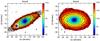 |
Fig. A.1 NGC 6762 (left panel) and NGC 5966 (right panel): the vertical color bar indicates (from the center outwards) the irregular annuli used for deriving radial profiles in Fig. 7. The overlaid contours are computed from SDSS g band images and go from 18 to 23.5 mag/◻″in steps of 0.5 mag. |
All Tables
Observed emission line fluxes in units of 10-16 erg cm-2 s-1 and physical properties from different apertures for NGC 6762.
Observed emission line fluxes in units of 10-16 erg cm-2 s-1 and physical properties from different apertures for NGC 5966.
All Figures
|
Fig. 1 Left panel: three-color, g, r, and i, composite SDSS image of NGC 6762. Foreground sources that have been disregarded in the subsequent spectral modeling and analysis are marked by crosses. Contours delineate an extremely faint spiral feature with a projected size of 31′′ × 9′′ disclosed by unsharp masking in the bulge of the galaxy. Right panel: SDSS color composite of NGC 5966 with contours from an unsharp masked image delineating a faint bar-like feature centered at the nucleus. North is up and east to the left in both images. |
| In the text | |
|
Fig. 2 NGC 6762: the panels to the left and right illustrate the main output from spectral synthesis in the blue and red spectral range, respectively, for a single spaxel in the brightest nuclear zone (top panels) and in the fainter periphery of the galaxy (~10′′ from the nucleus; bottom panels). The red and blue lines correspond to the observed and modeled stellar spectrum, respectively. By subtracting the latter from the former we obtain the pure nebular emission line spectrum (black). The spectra are offset in arbitrary units (au) for the sake of clarity. |
| In the text | |
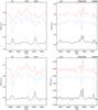 |
Fig. 3 NGC 5966: the same as Fig. 2. |
| In the text | |
|
Fig. 4 Maps of the emission from NGC 6762. Upper row from left to right: the stellar component distribution as traced by a continuum map made from the median flux between 6390–6490 Å, a spectral region free of line emission (“pure continuum”); the EW(Hα); Hβ; [Oiii]λ5007. Bottom row from left to right: [Oi]λ6300; Hα; [Nii]λ6584; [Sii]λ6717, 6731. All maps are presented in logarithmic scale to emphasize the relevant morphological features. Flux units are 10-16 erg cm-2 s-1. The axis origin (i.e. the center of the PPak bundle) is marked with a cross. Contours corresponding to the stellar continuum map are overplotted on all maps for reference. The contour corresponding to the minimun level is − 1.70 dex and the interval between contours is 0.25 dex. North is up and east to the left. The pixel size is 1″ (~217 pc at our assumed distance to NGC 6762 of 45 Mpc). A bar showing the physical scale of 5 kpc is plotted at the lower righthand corner in the continuum map. |
| In the text | |
|
Fig. 5 Maps of the emission from NGC 5966. The panels show the same maps as outlined in Fig. 4. See the caption to that figure for details. The pixel size (1″) corresponds to ~334 pc at our assumed distance to NGC 5966 of 69 Mpc. |
| In the text | |
|
Fig. 6 Emission line ratio maps for NGC 6762 (top row) and NGC 5966 (bottom row). All maps are in logarithmic scale. The label at the top of each map indicates what emission line ratios are being displayed. The contours, linear scale, and orientation are the same as in Figs. 4 and 5. |
| In the text | |
|
Fig. 7 Radial distribution of the [Oiii]λ5007/Hβ (triangle), [Nii]λ6584/Hα (square), and Hβpred./Hβobs. (cross; this ratio is discussed in Sect. 7) for NGC 6762 (left panel) and NGC 5966 (right panel). |
| In the text | |
|
Fig. 8 Diagnostic diagrams for NGC 6762. From left to right: log ([Oiii]λ5007/Hβ) vs. log ([Nii]λ6584/Hα), log ([Oiii]λ5007/Hβ) vs. log ([Sii]λ6731,6717/Hα) and log ([Oiii]λ5007/Hβ) vs. log ([Oi]λ6300/Hα). The upper and bottom rows show the spaxels with F(Hα)/F(Hα)peak ≤ 0.20 and 0.20 ≲ F(Hα)/F(Hα)peak ≲ 1.00, respectively. The black solid curve (in all three panels) is the theoretical maximum starburst model from Kewley et al. (2001), devised to isolate objects whose emission line ratios can be accounted for by the photoionization by massive stars (below and to the left of the curve) from those where some other source of ionization is required. The black-dashed curves in the [Sii]λ6731,6717/Hα and [Oi]λ6300/Hα diagrams represent the Seyfert-LINER dividing line from Kewley et al. (2006) and transposed to the [Nii]λ6584/Hα by Schawinski et al. (2007). The predictions of different ionization models for ionizing the gas are overplotted in each diagram. The red lines represent the shock grids of Allen et al. (2008) with solar metallicity and preshock magnetic field B = 1.00 μG. For the grid of shock models, the solid lines show models with increasing shock velocity Vs = 100, 200, 300, 1000 km s-1, and dotted lines the grids with densities ne from 0.1 cm-3 to 100 cm-3. Grids of photoionization by an AGN (Groves et al. 2004) are indicated by green curves, with ne = 100 cm-3 and a power-law spectral index of − 1.4. The corresponding dashed-lines show models for Z = Z⊙ and Z = 2 Z⊙ (from left to right), and solid lines trace the ionization parameter log U, which increases with the [Oiii]λ5007/Hβ ratio from log U = −3.6, − 3.0, 0.0. We downloaded the shock and AGN grids from the web page http://www.strw.leidenuniv.nl/~brent/itera.html. The boxes show the predictions of photoionization models by pAGB stars for Z = Z⊙ and a burst age of 13 Gyr (Binette et al. 1994). |
| In the text | |
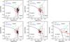 |
Fig. 9 Diagnostic diagrams for NGC 5966. Curves as in Fig. 8. |
| In the text | |
|
Fig. 10 EW(Hα) vs. log([Nii]λ6584/Hα) for NGC 6762. The left and right panels show the spaxels with F(Hα)/F(Hα)peak ≤ 0.20 and 0.20 ≲ F(Hα)/F(Hα)peak ≲ 1.00, respectively. SF = pure star-forming galaxies; sAGN = strong AGN; wAGN = weak AGN; RG = retired galaxies. The dividing lines are transpositions of the SF/AGN borders from Kewley et al. (2001, 2006) and Stasińska et al. (2006), and the Kewley et al. (2006) Seyfert/LINER division (see Cid Fernandes et al. 2010). |
| In the text | |
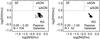 |
Fig. 11 EW(Hα) vs. log([Nii]λ6584/Hα) for NGC 5966. Labels as in Fig. 10. |
| In the text | |
|
Fig. 12 Kinematics maps of NGC 6762 (top row) and NGC 5966 (bottom row): stellar velocity field (left panels), corrected velocity dispersion maps (middle panels) and radial velocity maps (right panels), as measured from Hα. The contours, orientation, and linear scale are the same as in Figs. 4 and 5. |
| In the text | |
|
Fig. A.1 NGC 6762 (left panel) and NGC 5966 (right panel): the vertical color bar indicates (from the center outwards) the irregular annuli used for deriving radial profiles in Fig. 7. The overlaid contours are computed from SDSS g band images and go from 18 to 23.5 mag/◻″in steps of 0.5 mag. |
| In the text | |
Current usage metrics show cumulative count of Article Views (full-text article views including HTML views, PDF and ePub downloads, according to the available data) and Abstracts Views on Vision4Press platform.
Data correspond to usage on the plateform after 2015. The current usage metrics is available 48-96 hours after online publication and is updated daily on week days.
Initial download of the metrics may take a while.