| Issue |
A&A
Volume 540, April 2012
|
|
|---|---|---|
| Article Number | A82 | |
| Number of page(s) | 9 | |
| Section | Planets and planetary systems | |
| DOI | https://doi.org/10.1051/0004-6361/201118247 | |
| Published online | 29 March 2012 | |
Evidence for enhanced chromospheric Ca II H and K emission in stars with close-in extrasolar planets⋆
1 Department of Theoretical Physics and Astrophysics, Masaryk University, Kotlářská 2, 61137 Brno, Czech Republic
e-mail: This email address is being protected from spambots. You need JavaScript enabled to view it.
2 Astronomical Institute, Slovak Academy of Sciences, 05960 Tatranská Lomnica, Slovak Republic
e-mail: This email address is being protected from spambots. You need JavaScript enabled to view it.
Received: 11 October 2011
Accepted: 13 February 2012
Abstract
Context. The planet-star interaction is manifested in many ways. It has been found that a close-in exoplanet causes small but measurable variability in the cores of a few lines in the spectra of several stars, which corresponds to the orbital period of the exoplanet. Stars with and without exoplanets may have different properties.
Aims. The main goal of our study is to search for the influence that exoplanets might have on atmospheres of their host stars. Unlike the previous studies, we do not study changes in the spectrum of a host star or differences between stars with and without exoplanets. We aim to study a large number of stars with exoplanets and the current level of their chromospheric activity and to look for a possible correlation with the exoplanetary properties.
Methods. To analyse the chromospheric activity of stars, we exploited our own⋆⋆ and publicly available archival spectra⋆⋆⋆, measured the equivalent widths of the cores of Ca II H and K lines, and used them to trace their activity. Subsequently, we searched for their dependence on the orbital parameters and the mass of the exoplanet.
Results. We found statistically significant evidence that the equivalent width of the Ca II K line emission and log R'HK activity parameter of the host star varies with the semi-major axis and mass of the exoplanet. Stars with Teff ≤ 5500 K having exoplanets with semi-major axis a ≤ 0.15 AU (Porb ≤ 20 days) have a broad range of Ca II K emissions and much stronger emission in general than stars at similar temperatures but with higher values of semi-major axes. The Ca II K emission of cold stars (Teff ≤ 5500 K) with close-in exoplanets (a ≤ 0.15 AU) is also more pronounced for more massive exoplanets.
Conclusions. The overall level of the chromospheric activity of stars may be affected by their close-in exoplanets, and stars with massive close-in exoplanets may be more active.
Key words: planets and satellites: general / planets and satellites: magnetic fields / planet-star interactions / stars: chromospheres / stars: magnetic field / planetary systems
Table 1 is available in electronic form at http://www.aanda.org
2.2 m ESO/MPG telescope, Program 085.C-0743(A).
This research has made use of the Keck Observatory Archive (KOA), which is operated by the W. M. Keck Observatory and the NASA Exoplanet Science Institute (NExScI), under contract with the National Aeronautics and Space Administration.
© ESO, 2012
1. Introduction
There is a wide variety of interactions that may occur between a close-in planet and its host star: evaporation of the planet (Vidal-Madjar et al. 2003; Hubbard et al. 2007); precession of the periastron due to the general relativity, tides, or other planets (Jordán & Bakos 2008); synchronization and circularization of the planet’s rotation and orbit, strong irradiation of the planet, and its effect on the planet radius (Guillot & Showman 2002; Burrows et al. 2007); atmosphere or stratosphere (Hubeny et al. 2003; Burrows et al. 2008; Fortney et al. 2008). However, it is not only the planet that suffers from this interaction. Hot Jupiters also raise strong tides on their parent stars, and some of the stars can become synchronized as well. Dissipation of the tides can lead to an extra heating of the stellar atmosphere. Magnetic field of the exoplanet may interact with the stellar magnetic structures in a very complicated manner that is not understood very well and which is a subject of recent studies (Cuntz et al. 2000; Rubenstein & Schaefer 2000; Ip et al. 2004; Lanza 2008). Such interaction might be observed mainly in the chromospheres and coronae of the parent stars.
The planet-star interaction is currently examined across the whole energy spectrum beginning from X-rays to the radio waves and from the ground, as well as from the space. A planet-induced X-ray emission in the system HD 179949 was observed by Saar et al. (2008). On the other hand, the search for correlation between X-ray luminosity and exoplanetary parameters (Kashyap et al. 2008; Poppenhaeger & Schmitt 2011) has revealed very contradictory results. Based on the observations in the optical region, Shkolnik et al. (2005, 2008) have discovered variability in the cores of Ca II H and K, Hα and Ca II IR triplet in a few exoplanet host stars induced by the exoplanet.
Ca II H and K lines (3933.7 and 3968.5 Å) are one of the best indicators of stellar activity observable from the ground (Wilson 1968). These lines are very strong, and their core is formed in the chromosphere of the star. For quantitative assessment of chromospheric activity of stars of different spectral types, the chromosphere emission ratio  (the ratio of the emission from the chromosphere in the cores of the Ca II H and K lines to the total bolometric emission of the star) was introduced by Noyes et al. (1984). High values mean higher activity.
Knutson et al. (2010) find a correlation between the presence of the exoplanetary stratosphere and the Ca II H and K activity index of the star. Consequently, Hartman (2010) find a correlation between the surface gravity of Hot Jupiters and the stellar activity.
Recently, Canto Martins et al. (2011) have analysed the sample of stars with and without extrasolar planets. They searched for a correlation between planetary parameters and the parameter but did not reveal any convincing proof for enhanced planet-induced activity in the chromosphere of the stars. On the other hand, Gonzalez (2011) claims that stars with exoplanets have lower vsini and values (i.e. less activity) than stars without exoplanets.
In this paper, we search for possible correlations between the chromospheric activity of the star and properties of exoplanets. The equivalent width (EQW) of Ca II K line emission is used as an indicator of the level of chromospheric activity of the parent star.
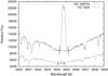 |
Fig. 1 Illustration of the Ca II K line in two different stars. We measured only the equivalent width of core of the line with the central reversal. By definition, EQW is negative for emission and positive for absorption. |
2. Observation and data
Stellar spectra used in our analysis originate from two different sources. The main source is the publicly available Keck HIRES spectrograph archive. These spectra have a typical resolution of up to 85 000. We carefully selected only those spectra with the signal-to-noise ratio high enough to measure the precise EQW of Ca II K emission.
These data were accompanied by our own observations of several stars (HD 179949, HD 212301, HD 149143, and Wasp-18) with a close-in exoplanet. We obtained these data with the FEROS spectrograph mounted on the 2.2 m ESO/MPG telescope (night 18/19.9.2010). Spectra were reduced with a standard procedure using the IRAF package1. These data are marked in all plots as red squares. We measured the EQW (in Å) of the central reversal in the core of Ca II K from all spectra using IRAF (see Fig. 1). This plot illustrates a placement of the pseudocontinuum in our measurements. The advantage of using such simple EQW measurements is that they are defined on a short spectral interval that is about 1 Å wide. Consequently, they are not very sensitive to the various calibrations (continuum rectification, blaze function removal) inherent in the echelle spectroscopy. For comparison, the index relies on the information from four spectral channels covering about a 100 Å wide interval. If extracted from echelle spectra, it is much more sensitive to a proper flux calibration and subject to added uncertainties.
The sample of the data contains 206+4 stars with extrasolar planets in the temperature range of approx. 4500 to 6600 K. The semi-major axes of the exoplanets lie in the interval 0.016–5.15 AU. Table 1 lists the parameters of exoplanetary systems used in the study.
For comparison with our EQW values, we also used the parameter taken from the works of Wright et al. (2004), Knutson et al. (2010), and Isaacson & Fischer (2010).
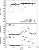 |
Fig. 2 Top: dependence of the equivalent width of the Ca II K emission on temperature of the parent star. Empty triangles denote exoplanetary systems with a ≤ 0.15 AU, full triangles are systems with a > 0.15 AU, and red squares are our data from FEROS. Emission and chromospheric activity increase with decreasing temperature. Cooler stars (Teff ≤ 5500 K) with close-in planets are more active than stars with more distant planets. Middle: statistical Student’s t-test (empty circles) and Kolmogorov-Smirnov test (full circles) show whether the two distributions are the same. Bottom: the same statistical tests performed on systems discovered by the RV technique alone. |
3. Statistical analysis and results
We start by exploring the dependence of the EQW of Ca II K emission on the effective temperature of the star. This is illustrated in the top panel of Fig. 22. One can see that the EQW decreases; i.e., core emission increases towards lower temperatures. Part of the reason for this behaviour is that the photospheric flux at the core of the Ca II K line is lower for cooler stars than for hotter stars. At the same time, the data points that stand for stars with Teff > 5500 K show only a narrow spread of Ca II K EQWs, while cooler stars have a broad range of these values. This means that we should focus on the cooler stars.
In the next step, we distinguish between the close-in and distant exoplanets. This is also shown in Fig. 2 where planets with semi-major axes that are shorter/longer than 0.15 AU have different symbols. One can see that stars with close-in planets clearly tend to have higher Ca II K emission (lower EQWs) than stars with distant planets. To verify whether this finding is statistically significant, we performed two statistical tests on these two data samples (close-in vs distant planets). The first one was the Student’s t-test, which determines whether the means of these two samples are equal. The other test was the Kolmogorov-Smirnov test, which we used to determine whether the two groups originate in the same population. We selected a running window that is 400 K wide and that runs along the x-axis (temperature) in steps of 50 K. Consequently, we performed the statistical tests on the two samples of stars within the current window and plot the result versus the centre of the current window. The middle panel of Fig. 2 shows the resulting probability (as a function of temperature) that the two samples have the same mean or originate in the same population. A low value of probability means that the two samples are different. It can be seen (Fig. 2), that the difference between the stars with close-in and distant exoplanets is statistically significant for cooler stars with Teff ≤ 5500 K.
However, while most of the distant exoplanets were discovered by the radial velocity (RV) measurements, many of the close-in planets were discovered by transits. The two techniques may have very different criteria for selecting the exoplanetary candidates, and especially the RV measurements concentrate on low-activity stars. That is why in the bottom panel of Fig. 2, we only included the stars with exoplanets discovered by the RV technique in the statistics. On this reduced data sample, we performed the same statistical tests as in the previous case, by choosing the same size step and the running window. Even if the transit data are excluded, the tests show a significant difference between the stars with close-in and distant exoplanets.
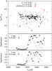 |
Fig. 3 Top: dependence of the activity index |
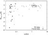 |
Fig. 4 Dependence of the equivalent width of Ca II K emission on the semi-major axis. Included are only systems with Teff ≤ 5500 K. Empty triangles are exoplanetary systems discovered by the RV technique, full triangles are systems discovered by transit method. |
To verify these trends, we also explored the parameter. This parameter does not show the strong temperature dependence (Fig. 3). When we distinguish the stars with close-in exoplanets (a ≤ 0.15 AU) from stars with distant exoplanets (a > 0.15 AU) using different symbols, we observed the same tendency as before. Namely, stars with close-in planets show a wider range of values than stars with distant planets. Cooler stars (Teff ≤ 5500 K) with close-in planets have higher values of and thus higher chromospheric activity. The difference between stars with close-in and distant planets is statistically significant for Teff ≤ 5500 K which is illustrated by the Student’s t-test and Kolmogorov-Smirnov test in the middle panel of Fig. 3. The bottom panel of the figure depicts the same tests applied to the systems discovered by the RV technique only and indicates that the difference is statistically significant even though the sample consists of stars with planets detected by a single technique. In this figure, we used the same kind of analysis within a running window, as before.
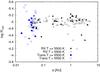 |
Fig. 5 Dependence of the activity index |
It appears that the semi-major axis of the innermost planet around a star is in some way connected with the chromospheric activity of the star. In the next step, we therefore explore the dependence of the activity on the semi-major axis a. This dependence is illustrated in Fig. 4, which displays the results we measured – EQW of Ca II K emission as a function of the semi-major axis. Following our findings above, we selected only systems with Teff ≤ 5500 K. One can clearly see two distinctive populations there. Stars with close-in exoplanets with a ≤ 0.15 AU have a broad range of Ca II K emission while stars with distant planets (a > 0.15 AU) have a narrow range of weak Ca II K emission. Again, we distinguish between stars with planets discovered by the RV and transit methods. A significant fraction of close-in planets were discovered by the RV method. Apparently, some stars with close-in exoplanets (but not all of them) have high Ca II K emission. Unfortunately, this finding may be affected by selection biases. (It is more difficult to detect distant planets around active stars.)
To verify this behaviour, we also explored the parameter as a function of the semi-major axis. This is illustrated in Fig. 5. This figure also shows a clear distinction between the stars with close-in planets with semi-major axis less than 0.15 AU and stars with distant planets. Stars with close-in exoplanets generally have higher scatter in the values than stars with distant planets. This is mainly caused by hotter stars with transiting exoplanets. Once we concentrate only on cold stars with planets detected by the RV technique there might be a trend for stars with close-in planets to have higher values than stars with distant planets, but it is not as pronounced as in EQW measurements. At the same time, there is no strong correlation with the semi-major axis for a ≤ 0.15 AU.
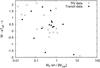 |
Fig. 6 Dependence of the modified equivalent width of Ca II K emission on planet mass. Only stars with Teff ≤ 5500 K and a ≤ 0.15 AU are considered. Modified equivalent width is equivalent width corrected for strong temperature dependence. By definition, the EQW is negative for emission. Consequently, lower values mean higher emission and higher chromospheric activity. Chromospheric activity of stars with more massive planets is higher than in those with less massive planets. Empty triangles denote stars with planets detected by the RV method, full triangles the transit method. |
However, what is it that causes the high range of values of Ca II K emission for cold stars with close-in planets? Is it due dependence on time? If so, on what timescales: the timescale of the planet orbital period, stellar activity cycle, age of the star, or something else? Is there any other parameter/process that affects the stellar chromosphere? We explored whether it may come from the eccentricity of the orbit but we did not find any convincing evidence for the eccentricity effect. If there is a dependence of the Ca II K emission on the semi-major axis of the planet, there ought to be some dependence on the mass mp of the planet (or its magnetic field) as well. This dependence would have to be continuously reduced in case of sufficiently small planets. Unfortunately, we know only mpsini for most of the extrasolar planets. Nevertheless, we select all stars with temperatures T ≤ 5500 K and with semi-major axis a ≤ 0.15 AU and fit EQWs of the Ca II K emission by the following function:  (1)We found the following coefficients: a = 3.65 × 10⁻³ ± 5.7 × 10⁻⁴,b = −0.392 ± 0.097 and c = −20.4 ± 2.9. The a coefficient is significant beyond 6σ, so temperature dependence is very clear. However, the b coefficient is also significant beyond 4σ, and it indicates the statistically significant correlation of the chromospheric activity with the mass of the planet. We applied statistical F-test to justify the usage of additional parameter (planet mass) in the above mentioned fitting procedure. The test shows that the significance of the 3-parameter fit (Eq. (1)) over the 2-parameter fit W(Teff) = aTeff + c is 0.003, which is below the common 0.05 value (2σ).
These results are illustrated in Fig. 6, where we plot the modified equivalent width of the Ca II K emission as a function of mpsini, showing stars with planets detected by RV and transit methods. The modified equivalent width is EQW corrected for the strong temperature dependence, namely EQW − aTeff − c. Lower values mean higher emission, and thus the host stars with more massive planets show more chromospheric activity. Unfortunately, this correlation might also be affected by the selection effect so that it is more difficult to detect a less massive planet around a more active star.
If our findings based on the Ca II K emission are true, than one can ask: how this planet-star interaction works and why it operates up to a = 0.15 AU. If it was caused by the tides of the planet, one would expect that the stellar activity would gradually decrease with a, which may not be the case. We suggest that it may be due to the magnetic interaction that scales with the magnetic field of the planet. This magnetic field may be very sensitive to the rotation profile of the planet, which is a subject to strong synchronization. Bodenheimer et al. (2001) suggest that exoplanets with semi-major axis a ≤ 0.15 AU are most probably synchronized.
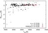 |
Fig. 7 Dependence of the equivalent width of Ca II H emission on the temperature of the star. Empty triangles are exoplanetary systems with a ≤ 0.15 AU, full triangles are systems with a > 0.15 AU, and red squares are our data from FEROS. |
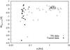 |
Fig. 8 Dependence of the equivalent width of Ca II H emission on the semi-major axis. Empty triangles are exoplanetary systems discovered by RV technique, full triangles are systems discovered by transit method. |
4. Conclusions
We have found statistically significant evidence that the EQW of the Ca II K emission in the spectra of planet host stars, as well as their activity index, depends on the semi-major axis of the exoplanet. Stars with close-in planets (a ≤ 0.15 AU) generally have higher Ca II K emission than stars with more distant
planets. This means that a close-in planet may affect the level of the chromospheric activity of its host star and might heat the chromosphere of the star. This process operates up to the orbital period of about 20 days. Moreover, we have found statistically significant evidence that the Ca II K emission of the host star (for Teff ≤ 5500 K and a ≤ 0.15 AU) increases with the mass of the planet. These trends may be affected by selection effects and should be revisited when less biased sample of stars with planets becomes available.
Online material
Parameters of exoplanetary systems.
2.2 m ESO/MPG telescope, Program 085.C-0743(A).
This research has made use of the Keck Observatory Archive (KOA), which is operated by the W. M. Keck Observatory and the NASA Exoplanet Science Institute (NExScI), under contract with the National Aeronautics and Space Administration.
Acknowledgments
We thank the anonymous referee for important comments and suggestions on the manuscript. This work has been supported by grant GA ČR GD205/08/H005, Student Project Grant at MU MUNI/A/0968/2009, the National scholarship programme of Slovak Republic, and by VEGA 2/0094/11, VEGA 2/0078/10 and VEGA 2/0074/09. We want to thank Tomáš Henych and Markéta Hynešová for fruitful discussion.
References
- Bodenheimer, P., Lin, D. N. C., & Mardling, R. A. 2001, ApJ, 548, 466 [NASA ADS] [CrossRef] [Google Scholar]
- Burrows, A., Hubeny, I., Budaj, J., & Hubbard, W. B. 2007, ApJ, 661, 502 [NASA ADS] [CrossRef] [Google Scholar]
- Burrows, A., Budaj, J., & Hubeny, I. 2008, ApJ, 678, 1436 [NASA ADS] [CrossRef] [Google Scholar]
- Canto Martins, B. L., Das Chagas, M. L., Alves, S., et al. 2011, A&A, 530, A73 [NASA ADS] [CrossRef] [EDP Sciences] [Google Scholar]
- Cuntz, M., Saar, S. H., & Musielak, Z. E. 2000, ApJ, 533, L151 [NASA ADS] [CrossRef] [PubMed] [Google Scholar]
- Fortney, J. J., Lodders, K., Marley, M. S., & Freedman, R. S. 2008, ApJ, 678, 1419 [NASA ADS] [CrossRef] [Google Scholar]
- Gonzalez, G. 2011, MNRAS, 416, L80 [NASA ADS] [CrossRef] [Google Scholar]
- Guillot, T., & Showman, A. P. 2002, A&A, 385, 156 [NASA ADS] [CrossRef] [EDP Sciences] [Google Scholar]
- Hartman, J. D. 2010, ApJ, 717, L138 [NASA ADS] [CrossRef] [Google Scholar]
- Hubbard, W. B., Hattori, M. F., Burrows, A., Hubeny, I., & Sudarsky, D. 2007, Icarus, 187, 358 [NASA ADS] [CrossRef] [Google Scholar]
- Hubeny, I., Burrows, A., & Sudarsky, D. 2003, ApJ, 594, 1011 [NASA ADS] [CrossRef] [Google Scholar]
- Ip, W.-H., Kopp, A., & Hu, J.-H. 2004, ApJ, 602, L53 [NASA ADS] [CrossRef] [Google Scholar]
- Isaacson, H., & Fischer, D. 2010, ApJ, 725, 875 [NASA ADS] [CrossRef] [Google Scholar]
- Jordán, A., & Bakos, G. Á. 2008, ApJ, 685, 543 [NASA ADS] [CrossRef] [Google Scholar]
- Kashyap, V. L., Drake, J. J., & Saar, S. H. 2008, ApJ, 687, 1339 [NASA ADS] [CrossRef] [Google Scholar]
- Knutson, H. A., Howard, A. W., & Isaacson, H. 2010, ApJ, 720, 1569 [NASA ADS] [CrossRef] [Google Scholar]
- Lanza, A. F. 2008, A&A, 487, 1163 [NASA ADS] [CrossRef] [EDP Sciences] [Google Scholar]
- Noyes, R. W., Hartmann, L. W., Baliunas, S. L., Duncan, D. K., & Vaughan, A. H. 1984, ApJ, 279, 763 [NASA ADS] [CrossRef] [Google Scholar]
- Poppenhaeger, K., & Schmitt, J. H. M. M. 2011, ApJ, 735, 59 [NASA ADS] [CrossRef] [Google Scholar]
- Rubenstein, E. P., & Schaefer, B. E. 2000, ApJ, 529, 1031 [NASA ADS] [CrossRef] [Google Scholar]
- Saar, S. H., Cuntz, M., Kashyap, V. L., & Hall, J. C. 2008, in IAU Symp. 249, ed. Y.-S. Sun, S. Ferraz-Mello, & J.-L. Zhou, 79 [Google Scholar]
- Shkolnik, E., Walker, G. A. H., Bohlender, D. A., Gu, P., & Kürster, M. 2005, ApJ, 622, 1075 [NASA ADS] [CrossRef] [Google Scholar]
- Shkolnik, E., Bohlender, D. A., Walker, G. A. H., & Collier Cameron, A. 2008, ApJ, 676, 628 [NASA ADS] [CrossRef] [Google Scholar]
- Vidal-Madjar, A., Lecavelier des Etangs, A., Désert, J.-M., et al. 2003, Nature, 422, 143 [NASA ADS] [CrossRef] [PubMed] [Google Scholar]
- Wilson, O. C. 1968, ApJ, 153, 221 [NASA ADS] [CrossRef] [Google Scholar]
- Wright, J. T., Marcy, G. W., Butler, R. P., & Vogt, S. S. 2004, ApJS, 152, 261 [NASA ADS] [CrossRef] [Google Scholar]
All Tables
All Figures
|
Fig. 1 Illustration of the Ca II K line in two different stars. We measured only the equivalent width of core of the line with the central reversal. By definition, EQW is negative for emission and positive for absorption. |
| In the text | |
|
Fig. 2 Top: dependence of the equivalent width of the Ca II K emission on temperature of the parent star. Empty triangles denote exoplanetary systems with a ≤ 0.15 AU, full triangles are systems with a > 0.15 AU, and red squares are our data from FEROS. Emission and chromospheric activity increase with decreasing temperature. Cooler stars (Teff ≤ 5500 K) with close-in planets are more active than stars with more distant planets. Middle: statistical Student’s t-test (empty circles) and Kolmogorov-Smirnov test (full circles) show whether the two distributions are the same. Bottom: the same statistical tests performed on systems discovered by the RV technique alone. |
| In the text | |
|
Fig. 3 Top: dependence of the activity index |
| In the text | |
|
Fig. 4 Dependence of the equivalent width of Ca II K emission on the semi-major axis. Included are only systems with Teff ≤ 5500 K. Empty triangles are exoplanetary systems discovered by the RV technique, full triangles are systems discovered by transit method. |
| In the text | |
|
Fig. 5 Dependence of the activity index |
| In the text | |
|
Fig. 6 Dependence of the modified equivalent width of Ca II K emission on planet mass. Only stars with Teff ≤ 5500 K and a ≤ 0.15 AU are considered. Modified equivalent width is equivalent width corrected for strong temperature dependence. By definition, the EQW is negative for emission. Consequently, lower values mean higher emission and higher chromospheric activity. Chromospheric activity of stars with more massive planets is higher than in those with less massive planets. Empty triangles denote stars with planets detected by the RV method, full triangles the transit method. |
| In the text | |
|
Fig. 7 Dependence of the equivalent width of Ca II H emission on the temperature of the star. Empty triangles are exoplanetary systems with a ≤ 0.15 AU, full triangles are systems with a > 0.15 AU, and red squares are our data from FEROS. |
| In the text | |
|
Fig. 8 Dependence of the equivalent width of Ca II H emission on the semi-major axis. Empty triangles are exoplanetary systems discovered by RV technique, full triangles are systems discovered by transit method. |
| In the text | |
Current usage metrics show cumulative count of Article Views (full-text article views including HTML views, PDF and ePub downloads, according to the available data) and Abstracts Views on Vision4Press platform.
Data correspond to usage on the plateform after 2015. The current usage metrics is available 48-96 hours after online publication and is updated daily on week days.
Initial download of the metrics may take a while.