| Issue |
A&A
Volume 539, March 2012
|
|
|---|---|---|
| Article Number | A40 | |
| Number of page(s) | 9 | |
| Section | Atomic, molecular, and nuclear data | |
| DOI | https://doi.org/10.1051/0004-6361/201118401 | |
| Published online | 22 February 2012 | |
Stark halfwidth trends along the homologous sequence of doubly ionized noble gases
1 Departamento de Física Teórica, Atómica y Óptica, Universidad de Valladolid, 47071 Valladolid, Spain
e-mail: This email address is being protected from spambots. You need JavaScript enabled to view it.
2 Faculty of Sciences, Department of Physics, Trg Dositeja Obradovića 4, 21000 Novi Sad, Serbia
Received: 4 November 2011
Accepted: 28 December 2011
Abstract
Aims. The aim of this work is to analyze the behavior of experimentally determined Stark halfwidths for (n − 1)d − np and ns − np transitions along the homologous sequence of doubly ionized noble gases.
Methods. We analyzed the Stark halfwidth trends including all available experimental data. Stark halfwidth results for the above mentioned transitions and corresponding multiplets were compared with the halfwidths calculated using the modified semiempirical formula (MSE) and the simplified modified semiempirical formula (SMSE). In case of Ne III the calculation made by semiclassical-perturbation formalism (SCPF) is also presented.
Results. Stark halfwidths corresponding to (n − 1)d − np and ns − np transitions have been analyzed along the homologous sequence of doubly ionized noble gases. For all multiplets observed in this work, the analysis shows that the halfwidths of the spectral lines belonging to the same transition show a similar trend along the homologous sequence. Stark halfwidths of ns − np transitions have a clearly increasing trend. On the other hand, for (n − 1)d − np transitions, there are not enough data to make a similar conclusion. This type of trend analysis can be useful for Stark halfwidth predictions and hence for spectroscopic diagnostics of astrophysical plasmas.
Key words: plasmas / atomic data / line: profiles
Present address: Instituto de Óptica, CSIC, 28006 Madrid, Spain.
© ESO, 2012
1. Introduction
Generally, investigating Stark broadening of noble gase ionic lines has a great importance for the spectroscopy of both laboratory and astrophysical plasmas (Reyna et al. 2009). The Stark parameter behavior along the homologous sequence can provide more information that is especially valuable for astrophysical spectroscopy. There are several astrophysical problems for which Stark broadening data are of great interest, such as abundance determination, calculation of stellar opacities (Iglesias et al. 1990), interpretation and modeling of stellar spectra, stellar atmosphere modeling (Werner 1984) and investigations, estimation of the radiation transfer through the stellar plasma, etc. Studying the spectral line shape has been additionally stimulated by the development of space astronomy, through which an extensive amount of spectroscopy information has been collected, and also through the development of software for stellar atmosphere simulations, such as TMAP (Werner et al. 2003), SMART (Sapar et al. 2009) etc., which need large amount of atomic and spectroscopic data. These parameters will be useful for a future development of stellar atmosphere and evolution models (Leitherer et al. 2010). In the spectra of O, B and A type stars, as well as white dwarfs, many singly and multiply charged ion lines have been observed (Peytremann 1972; Lanz et al. 1988; Popović et al. 1999). In the atmospheres of these stars, Stark broadening is the dominant pressure-broadening mechanism. In addition, Stark broadening may be important in the atmospheres of relatively cool stars, such as Sun. Ionized noble gases are detected in many astronomic spectra. All spectral lines from ultraviolet to infrared spectral region are of interest.
Neon is the most abundant element in the universe after H, He, O and C (Trimble 1991). Neon has also been observed in supernova ejecta (Thieleman et al. 1986; Woosley et al. 1988). Ne III lines have been identified in the spectrum of solar active region (Thomas & Neupert 1994). For this reason, the neon spectrum is much more used in astro-spectroscopy than the spectrum of argon, krypton and xenon. Lutz et al. (1998) and Thornley et al. (2000) used emission of Ne III/Ne II spectral lines to investigate massive star formation and evolution in starburst galaxies. Stark halfwidths of ultraviolet Ne II and Ne III lines of astrophysical interest were measured and calculated by Milosavljević et al. (2001) and Dimitrijević (2001), respectively. Ultraviolet Ne III spectral lines are specifically interesting in the NGC 3918 planetary nebulae (McLaughlin et al. 2000, 2002). Ne III is also present in the nucleus of the starburst galaxy NGC 253 and its immediate surroundings (Devost et al. 2004). Armus et al. (2004) used the ratio of some Ne II, III and V spectral lines for the electron density determination in the Markarian 1014, Markarian 463, and UGC 51011 galaxies, while Dale et al. (2006) and Hao et al. (2009) used Ne II and Ne III lines for spectral diagnostics of nuclear and extranuclear regions in nearby galaxies. Variability of the Ne III spectra and the X-ray emission give consistent results and suggest the presence of a companion star in a highly eccentric orbit in Eta Carinae. Spectra containing Ne III lines, acquired in the last years, are used to corroborate this hypothesis and analyze this interesting object (Nielsen et al. 2009; Mehner et al. 2010).
The Ne III and Ar III spectral lines were used for diagnostics of the ionized medium in the Galactic center (Lutz et al. 1996). Beirão et al. (2008) analyzed the infrared spectrum of the central region of the M82 galaxy. For this analysis they used, among others, Ne III and Ar III lines. The detection of high-excitation Ne III lines confirms the presence of very young massive stars in M82. With the help of starburst models, it is possible to use the Ne III/Ne II ratio to estimate the age of the massive clusters in the region. The Ar III infrared line was identified in eight nearby Seyfert galaxies (Hönig et al. 2008). Ar III emission lines are of particular interest in astrophysics as a diagnostic tool (Verner et al. 2005; Hora et al. 2006; Ennis et al. 2006). Electron temperature and abundances of planetary nebulae are obtained from Ar III spectral lines (Keenan et al. 1988). Otsuka et al. (2010) performed a comprehensive chemical abundance analysis of the planetary nebula BoBn 1. Among others, these authors used ultraviolet Ne III and visible Ar III spectral lines. These elements and their lines have also been found and analyzed in Eta Carinae (Damineli et al. 1998). Mehner et al. (2010) investigated the emission of the ultraviolet Ne III line (387.0 nm) and Ar III line ratio (311.0/519.3) using the data observed by the Hubble Space Telescope.
Péquignot & Baluteau (1994) identified krypton and xenon in the planetary nebula NGC 7072. The identification of heavy elements in the planetary nebulae IC 7027 stimulated the analysis of transition probabilities (Biémont et al. 1995) and collisional data (Schöning & Butler 1998) for Xe III ions, among others. Infrared and visible Kr III spectral lines have also been identified in planetary nebulae, as well as Ne III and Ar III lines (Dinerstein 2001; Sharpee et al. 2007; Sterling & Dinerstein 2008). Zhang et al. (2006) detected Kr III and Xe III visible spectral lines in the planetary nebulae IC 2501, IC 4191, NGC 2440 and NGC 7027. Roman-Lopes et al. (2009) used Ne III and Kr III spectral lines for the observation of young massive stars embedded in molecular clouds.
In addition to collecting the experimental data, we have analyzed regularities and systematic trends of the Stark parameters. Pittman & Konjević (1986) first started this analysis of experimental Stark broadening data along the homologous sequence of singly ionized noble gases. Similar investigations were conducted in papers by Miller et al. (1980) for other ionized atoms and by Dimitrijević et al. (1987) and Vitel et al. (1988) for neutral atoms. More details about the regularities and systematic trends of the Stark parameters are given in Peláez et al. (2010). Here, we analyzed Stark halfwidths, corresponding to (n − 1)d − np and ns − np transitions, along the homologous sequence of doubly ionized noble gases. We analyzed analogous spectral line halfwidths of homologous ions. “Analogous” indicates that the same type of transition has only the principal quantum number changed, while “homologous” indicates ions with the same electric charge and a similar energy level structure in the outer shells. Owing to these similarities, a gradual increase of the spectral line halfwidths, i.e., the systematic trend should be expected in these cases. For the analysis of (n − 1)d − np and ns − np transitions, the following references are available: Platiša et al. (1975), Konjević & Pittman (1987), Purić et al. (1988), Kobilarov & Konjević (1990), Uzelac et al. (1993), Djeniže et al. (1996), Iriarte et al. (1997), Romeo y Bidegain et al. (1998), Ahmad et al. (1998), Blagojević et al. (2000), Milosavljević et al. (2000, 2001), Seidel et al. (2001), Peláez et al. (2006), Bukvić et al. (2008), Peláez et al. (2009), Ćirišan et al. (2011) and Djurović et al. (2011).
2. Experimental data
Eighteen papers, mentioned above, report experimentally determined Stark halwidth data for doubly ionized noble gases. Basic data about the plasma sources, diagnostic techniques and plasma conditions are given in Table 1. In most experiments, a low-pressure pulsed arc was used as a plasma source; while in rest of experiments, a linear pinch was used. For each paper, we provide a list of the observed ions together with the estimate of the halfwidth experimental errors. Experimental errors from Seidel et al. (2001) are taken from the results graphically presented in the paper, while information about the experimental errors in the Iriarte et al. (1997) and Romeo y Bidegain et al. (1998) papers are missing. Relatively large experimental errors are estimated in the Peláez et al. (2009), Ćirišan et al. (2011) and Djurović et al. (2011) papers. Peláez et al. (2009) deal with low-intensity lines and their experimental error analysis is given in detail in the paper. Papers from Ćirišan et al. (2011) and Djurović et al. (2011) deal with very narrow spectral lines, between 10 and 20 pm, and the estimate of the errors is explained in Ćirišan et al. (2011).
Basic experimental data on plasma sources and plasma conditions for different experiments.
Because similar plasma sources were used we can compare the determined Stark halfwidth values along the homologous sequence of doubly ionized noble gases. However, the experiments were performed under different plasma conditions and different diagnostic techniques were used. From Table 1, one can see that the experiments were performed in a wide range of plasma electron density, from 0.20 × 10²³ m-3 to 27.20 × 10²³ m-3 and temperatures varied from 16 000 K to 110 000 K. The Stark halfwidth dependence on electron density is clearly linear. The Stark halfwidth dependence on electron temperature is a more delicate point. Theoretical predictions, for example semiempirical formula (Griem 1968) and modified semiempirical formula (Dimitrijević & Konjević 1980), give the  halfwidth dependence on electron temperature. It is necessary, in this case, to check this dependence because of the wide range of electron temperatures characterizing plasmas in different experiments. The widest range of temperature, 21 000 K to 110 000 K, is shown in Fig. 1 in case of Ar III. This is the best case for checking the Stark halfwidth-temperature dependence. In general, measured Stark halfwidhs show a temperature dependence and follow the calculated Stark halfwidth values. Calculations are based on modified semiempirical formula (Dimitrijević & Konjević 1980). We explain the dispersion of experimental points and two theoretical curves, presented in Fig. 1 by two solid lines, below. Here, we only aim to show that by using the dependence, one can indeed compare the results obtained for example at temperature of 20 000 K and at temperature of 100 000 K.
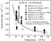 |
Fig. 1 Ar III Stark halfwidths for the 4s−4p transitions as a function of temperature at an electron density of 1023 m-3. |
3. Analysis of the Stark halfwidths for the (n − 1)d – np and ns − np transitions
Until today, only one paper, Konjević & Pittman (1987), analyzed the Stark halfwidth behavior along the homologous sequence of doubly ionized noble gases. The scarcity of available data did not allow a more comprehensive analysis of the halfwidth behavior at that time.
We analyzed the halfwidth data for the spectral lines belonging to the (n − 1)d − np and ns − np transitions where n = 3 for Ne III, n = 4 for Ar III, n = 5 for Kr III and n = 6 for Xe III. Stark halfwidth results for all available experimental data of doubly ionized noble gases from Ne III to Xe III are presented graphically in Figs. 2 to 5. For the analysis, we expressed the Stark halfwidths in angular frequency units (ω) to avoid the wavelength dependence. References used for this analysis are numbered in historical order. For the subsequent analysis, the reference numbers are the same as in Table 1, as are the symbols in all figures. Furthermore, to facilitate comparison the ordinate is the same in all figures from 2 to 5, and data are normalized to an electron density of 1.0 × 10²³ m-3 and to an average temperature, which is different for different ions.
Results for Ne III (Fig. 2) are taken from Konjević & Pittman (1987), Purić et al. (1988), Uzelac et al. (1993), Blagojević et al. (2000) and Milosavljević et al. (2001). Here one should notice that the 2d level does not exist for Ne III.
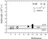 |
Fig. 2 Experimental Ne III Stark halfwidth data for the 3s − 3p transition. References: 2 – Konjević and Pittman (1987), 3 – Purić et al. (1988), 5 – Uzelac et al. (1993), 10 – Blagojević et al. (2000) and 12 – Milosavljević et al. (2001). Dotted lines represent theoretical results of SCPF calculation (Dimitrijevic 2001), solid lines represent data calculated with the MSE formula (Dimitrijević & Konjević 1980) and dashed lines represent data calculated with the SMSE formula (Dimitrijević & Konjević 1987). |
Results for Ar III (Fig. 3) are taken from Platiša et al. (1975), Konjević & Pittman (1987), Purić et al. (1988), Kobilarov & Konjević (1990), Djeniže et al. (1996), Bukvić et al. (2008) and Djurović et al. (2011). Results for Kr III (Fig. 4) are taken from Konjević & Pittman (1987), Ahmad et al. (1998), Milosavljević et al. (2000) and Ćirišan et al. (2011). Results for Xe III (Fig. 5) are taken from Konjević & Pittman (1987), Iriarte et al. (1997), Romeo y Bidegain et al. (1998), Seidel et al. (2001), Peláez et al. (2006, 2009).
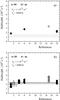 |
Fig. 3 Experimental Ar III Stark halfwidth data for a) 3d – 4p and b) 4s – 4p transitions. References: 1 – Platiša et al. (1975), 2 – Konjević & Pittman (1987), 3 – Purić et al. (1988), 4 – Kobilarov & Konjević (1990), 6 – Djeniže et al. (1996), 15 – Bukvić et al. (2008) and 18 – Djurović et al. (2011). Solid lines represent data calculated with the MSE formula (Dimitrijević & Konjević 1980) and dashed lines represent data calculated with the SMSE formula (Dimitrijević & Konjević 1987). |
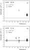 |
Fig. 4 Experimental Kr III Stark halfwidth data for the a) 4d − 5p and b) 5s − 5p transitions. References: 2 – Konjević & Pittman (1987), 9 – Ahmad et al. (1998), 11 – Milosavljević et al. (2000) and 17 – Ćirišan et al. (2011). Solid lines represent data calculated with the MSE formula (Dimitrijević & Konjević 1980) and dashed lines represent data calculated with the SMSE formula (Dimitrijević & Konjević 1987). |
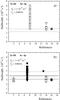 |
Fig. 5 Experimental Xe III Stark halfwidth data for the a) 5d − 6p and b) 6s − 6p transitions. References: 2 – Konjević & Pittman (1987), 7 – Iriarte et al. (1997), 8 – Romeo y Bidegain et al. (1998), 13 – Seidel et al. (2001), 14 – Peláez et al. (2006), 16 – Peláez et al. (2009). Solid lines represent data calculated with the MSE formula (Dimitrijević & Konjević 1980) and dashed lines represent data calculated with the SMSE formula (Dimitrijević & Konjević 1987). |
All above mentioned results published up to 2007 are critically reviewed in Konjević & Wiese (1976), Konjević et al. (1984), Konjević & Wiese (1990), Konjević et al. (2002) and Lesage (2009).
Two factors should be taken into account when analyzing the agreement of the experimentally obtained Stark halfwidths shown in Figs. 2 to 5. The first one is the experimental error of the obtained results. The second is the difference between the halfwidths of different lines belonging to the same transition array, or even to the same supermultiplet or multiplet. It was established in Wiese & Konjević (1982) that the Stark halfwidth values of the lines belonging to the same transition array may vary within a range of about ± 40%.
If we take into account both experimental errors and regularity established in Wiese & Konjević (1982), we can say that all measured Ne III line halfwidths belonging to the 3s − 3p transition agree well. The variation of the Stark halfwidth for different spectral lines shown in Fig. 2 is less than ± 20% in all cases. For Ar III case, both the 3d − 4p and 4s − 4p transition are considered. For the 3d − 4p transition, very few data exist (see Fig. 3a) and we can only say that the results vary by about ± 35% around the average value. There are more data and variations for the 4s − 4p transition array (Fig. 3b). The variation of the Stark halfwidth values in Platiša et al. (1975) and Konjević & Pittman (1987) is about ± 22%, in Kobilarov & Konjević (1990) is ± 12%, in Djeniže et al. (1996) is ± 16%, in Bukvić et al. (2008) is ± 21% and in Djurović et al. (2011) is ± 15%. There is only one result from Purić et al. (1988).
The situation for Kr III is similar; there are only few halfwidth results for the 4d − 5p and slightly more results for the 5s − 5p transition array (see Figs. 4a and b). There is only one halfwidth result from Milosavljević et al. (2000) and several results from Ćirišan et al. (2011) for the 4d − 5p transition (Fig. 4a). The results of Ćirišan et al. (2011) vary by about ± 15%. The Stark halfwidth variation for the 5s − 5p transition (Fig. 4b) is as follows: halfwidths from Konjević & Pittman (1987) vary by about ± 12%, those from Milosavljević et al. (2000) by ± 40% and those from Ćirišan et al. (2011) by ± 15%. If we exclude the two highest results from Milosavljević et al. (2000; see Fig. 4b), the variation of the other halfwidth results is about ± 20%. The smallest variation of halfwidth results comes from Ahmad et al. (1998) and is only about ± 4%. Ahmad et al. (1998) reported halfwidth values for only three lines, but they measured the halfwidth seven times for each line. The variation of the halfwidth value within seven measurements is about ± 16%.
For the 5d − 6p transitions of Xe III, the only data available are from Romeo y Bidegain et al. (1998) and Peláez et al. (2006, 2009; see Fig. 5a). Results from Peláez et al. (2006) show similar variation as in previous cases, about ± 25%. If we exclude the two highest values, the halfwidth variation is ± 12%. The largest variations come from data measured by Romeo y Bidegain et al. (1998), about ± 53%. In Fig. 5b, the halfwidth results for the 6s − 6p transition are shown. The Stark halfwidth data variation from Konjević & Pittman (1987) is about ± 15%, from Iriarte et al. (1997) ± 40% and from Peláez et al. (2006) ± 18%. The data from Peláez et al. (2009) show small variations, about ± 3%, but this is because of the small number of data. The same occurs with results from Seidel et al. (2001), where there are only two experimental points.
The largest variations are between the results of Iriarte et al. (1997) and Romeo y Bidegain et al. (1998) for the Xe III halfwidths. Furthermore, most of these halfwidth values are considerably higher than the halfwidth results of other authors (see Figs. 5a and b). The results from these two papers are discussed in detail in Peláez et al. (2006). One should also keep in the mind their very poor plasma diagnostic procedure (see Table 1). The rest of the halfwidth results for Ne III, Ar III, Kr III and Xe III lines and for the two (n − 1)d − np and ns − np transitions show variations lower than ± 40%, which is established as a normal variation for the Stark halfwidths of the lines belonging to the same transition array.
Present results (Figs. 2 to 5) are compared with calculated Stark halfwidth data. For that purpose, we used the modified semiempirical formula MSE (Dimitrijević & Konjević 1980) and the simplified modified semiempirical formula SMSE (Dimitrijević & Konjević 1987) which we discuss below. The best agreement with the calculated halfwidths for Ne III is obtained with data from Konjević & Pittman (1987), Purić et al. (1988) and Uzelac et al. (1993); for Ar III with data from Konjević & Pittman (1987) and Djurović et al. (2011) and close results from Kobilarov & Konjević (1990) and Djeniže et al. (1996); for Kr III the best agreement is obtained with data from Konjević & Pittman (1987) and Ćirišan et al. (2011) and, finally, for Xe III with data from Konjević & Pittman (1987) and Peláez et al. (2006, 2009). Taking into account experimental errors and calculation uncertainties, the experimental and theoretical data for all Ne III, Ar III, Kr III and Xe III lines for ns − np transition agree reasonably well, if we exclude results from Iriarte et al. (1997). The experimental results for the Ar III, Kr III and Xe III lines for the (n − 1)d − np transitions disagree quite obviously which is also true for the SMSE calculated data.
To generally analyze the Stark halfwidth behavior along the homologous sequence of doubly ionized noble gases, we present graphically the results in Fig. 6. Experimental results from Iriarte et al. (1997) and Romeo y Bidegain et al. (1998) are not included in Fig. 6 or in the following analysis because their experimental points are highly dispersed and their plasma diagnostics are poor. Our conclusion about the behavior of individual Stark halfwidth data is the same as mentioned above, but in addition one can see the increase of halfwidth values along the sequence more clearly. This increasing trend is not as obvious for the (n − 1)d − np transitions (Fig. 6a), partly due to the smaller number of available data for the analysis and partly due to the grater variation of data than for the ns − np transitions (Fig. 6b). To facilitate comparisons, all data are normalized to an electron temperature of 30 000 K. The theoretical data in Fig. 6 are presented in the same way as in previous figures, MSE calculations by solid line and SMSE calculation by dashed line. The experimental data of the (n − 1)d − np transition have higher values than the SMSE calculated data (Fig. 6a), while for the ns − np transitions the halfwidth data agree on average with the MSE calculations (Fig. 6b).
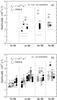 |
Fig. 6 Experimental Stark halfwidth data for the a) (n − 1)d − np and for b) ns − np transitions along the homologous sequence. References: 1 – Platiša et al. (1975), 2 – Konjević & Pittman (1987), 3 – Purić et al. (1988), 4 – Kobilarov & Konjević (1990), 5 – Uzelac et al. (1993), 6 – Djeniže et al. (1996), 9 – Ahmad et al. (1998), 10 – Blagojević et al. (2000), 11 – Milosavljević et al. (2000), 12 – Milosavljević et al. (2001), 13 – Seidel et al. (2001), 14 – Peláez et al. (2006), 15 – Bukvić et al. (2008), 16 – Peláez et al. (2009), 17 – Ćirišan et al. (2011) and 18 – Djurović et al. (2011). Solid lines represent data calculated with the MSE formula (Dimitrijević & Konjević 1980) and dashed lines represent data calculated with the SMSE formula (Dimitrijević & Konjević 1987). |
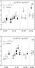 |
Fig. 7 Evolution of the Stark halfwidths a) for the (4S°)5S° − (4S°)5P and b) for (2D°)3D° − (2D°)3F multiplets belonging to the ns − np transitions. References: 1 – Platiša et al. (1975), 2 – Konjević & Pittman (1987), 3 – Purić et al. (1988), 5 – Uzelac et al. (1993), 6 – Djeniže et al. (1996), 9 – Ahmad et al. (1998), 11 – Milosavljević et al. (2000), 12 – Milosavljević et al. (2001), 13 – Seidel et al. (2001), 14 – Peláez et al. (2006), 15 – Bukvić et al. (2008), 17 – Ćirišan et al. (2011) and 18 – Djurović et al. (2011). Solid lines represent data calculated with the MSE formula (Dimitrijević & Konjević 1980). Only the average values of the MSE calculations are presented for each multiplet. |
In conclusion, the present Stark data show a regular behavior within the transition array, as established in Wiese & Konjević (1982), and in that sense they are valid for this type of analysis. At the same time, the increase in Stark halfwidth along the homologous sequence of doubly ionized noble gases is shown.
4. Analysis of the Stark halfwidths within the multiplets
For this type of analysis, only multiplets belonging to the ns − np transitions because of the large number of available experimental data.  and
and  multiplets with (4S°) and (2D°) parent terms, respectively, are considered. The comparison is shown in Figs. 7a and b.
The variation of the Stark halfwidths for lines belonging to the same multiplet are expected to be within a few percents according to Wiese & Konjević (1982). If we observe the data from different authors separately, the variation of experimental halfwidth results belonging to the multiplet along the sequence is less than ± 8% (Fig. 7a). This agrees with Wiese & Konjević (1982), if we take into account the experimental errors (see Table 1). Only the data from Platiša et al. (1975), for the Ar III lines show a larger variation: ± 19% around the average halfwidth value. To carry out an individual analysis of data of the Ne III to Xe III lines, it is more convenient to exclude the data sets showing a large difference compared to other results, and to calculated data. For Ar III, these results come from Platiša et al. (1975), for Kr III from Ahmad et al. (1998) and for Xe III from Seidel et al. (2001). In this case, the dispersion of the experimental data from all authors is about ± 22% for the Ne III lines, ±19% for the Ar III lines, ±6% for the Kr III and ±13% for the Xe III lines. These values are reasonable if one takes into account the experimental errors.
The variation of the experimental halfwidth results from different authors for the lines belonging to the multiplet along the sequence is less than ± 8% in most cases (Fig. 7b). There are only three halfwidth results from Purić et al. (1988) (Ne III case), two of them are very close and cannot be distinguished in Fig. 7b, but the dispersion of the results is within ± 14%. The same dispersion appears for the two data from Platiša et al. (1975) for Ar III, while the results from Djeniže et al. (1996) are within ± 20%. The Kr III results from Milosavljević et al. (2000) are within ± 13%. The rest of the results show variations lower than ± 8%. The analysis of all authors’ results for each element in the sequence shows a higher dispersion. For Ne III the dispersion is about ±32%, for Ar III even more, about ± 40%, slightly lower for Kr III, about ± 17% and a very low dispersion for Xe III, only ± 6%. The lowest dispersion of the halfwidth results for Xe III may be partly due to the small number of available experimental results. The largest disagreement with calculated Stark halfwidths appears for the Milosavljević et al. (2001) data for Ne III and for the Bukvić et al. (2008) data for Ar III.
5. Comparison of experimental and calculated Stark halfwidth data
In all previous figures, calculated Stark halfwidths are shown together with the experimental halfwidth values. As already mentioned, we used the modified semiempirical formula MSE (Dimitrijević & Konjević 1980) and the simplified modified semiempirical formula SMSE (Dimitrijević & Konjević 1987) for our calculation, see for details Peláez et al. (2010). All energy level data were taken from the NIST Atomic database. Dispersion of the calculated halfwidth values for the considered transition array is shown by two solid lines in Figs. 1 to 5. This dispersion is much lower than the dispersion of the experimental data for all considered results. Furthermore, in Figs. 3a to 5a only SMSE calculated results are presented. The MSE calculations were performed only if a complete set of perturbing levels data was available. For the (n − 1)d levels, some perturbing level data are missing in the database and therefore MSE data are missing in Figs. 3a to 6a. For Ne III the calculated results obtained by semiclassical-perturbation formalism SCPF are also presented (see Fig. 2). The SCPF results were taken from Dimitrijevic (2001). More details about the calculation procedure can be found in Milosavljevic et al. (2001).
In Fig. 8, the ratio between experimental and MSE calculated halfwidth values is shown for spectral lines of the multiplet. The lines for which experimental data were available for the analysis are given in Table 2. Most of the ratios range from 0.7 to 1.3. Only the results from Milosavljević et al. (2001) for Ne III, from Ahmad et al. (1998) for Kr III, and from Seidel et al. (2001) for Xe III show higher ratios, between 1.4 and 1.7.
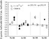 |
Fig. 8 Ratio of experimental and calculated Stark halfwidths. The symbols and references are the same as in Fig. 7a. |
Wavelengths of the spectral lines of the ns(4S°)5S° − np(4S°)5P multiplets.
It is possible to make an additional comparison between experimental and calculated results. Namely, it is possible to check the validity of normalization factor  (1)which is derived from simplified modified semiempirical formula (Dimitrijević & Konjević 1987). As it is shown by Konjević & Pittman (1987), the ratio
  (2)should be constant for the lines of the same homologous transition. In expressions (1) and (2),
  represents the effective principal quantum number, while lj is the orbital angular momentum quantum number of the desired transition with j = i and j = f for the upper and lower energy level, respectively. More explanations about this ratio and normalization factor are given in Peláez et al. (2010). The ratio of the Stark halfwidth values, expressed in angular units, over the normalization factor along the sequence is shown in Fig. 9. The average value of all present results is shown by a solid horizontal line.
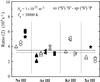 |
Fig. 9 Normalized halfwidth results along the sequence for |
Generally speaking, the Ne III normalized halfwidth results (Fig. 9) are higher than the other results. Interestingly the same behavior is shown by Ne II results for the singly ionized noble gas homologous sequence (Peláez et al. 2010). With the exception of Ne III results and taking into account the data dispersion, due to experimental errors, we can conclude that the introduced factor (1, 2) normalizes the results, i.e., it preserves a constant value of ratio (2). This is shown by the horizontal dashed line in Fig. 9.
6. Conclusions
We have analyzed the behavior of experimentally determined Stark halfwidths for the (n − 1)d − np and ns − np transitions along the homologous sequence of doubly ionized neon, argon, krypton, and xenon atoms. For this analysis, we used all experimental results available in the literature. To compare the data, which were obtained under different plasma conditions, they were normalized to the same electron density and temperature. It was shown that in spite of their intrinsic dispersion, experimental Stark halfwidth results follow the temperature dependence and show a regular behavior within multiplets or transition arrays, as established by Wiese & Konjević (1982). Furthermore, experimental halfwidths follow a trend of increasing values along the observed homologous sequence. The increase of the principal quantum number along the sequence leads to a reduction of the distances between the transition energy levels and their corresponding perturbing levels. The interaction of the transition energy levels with the perturbing levels is a function of both the closeness of the perturbing levels and their interaction strength. This confirms the behavior of Stark halfwidths along the homologous sequence described above. If there are some strong close perturbing levels, some irregularities may occur in the observed trend, but such cases have not been found in this analysis.
From Fig. 6, one could see that dispersion of the experimental data, in most cases, is higher than the estimated experimental errors in individual experiments. Furthermore, in some cases, data obtained in different experiments show large differences between each other and when compared to calculated results. If we ignore these few results, which clearly deviate from the others, we can say that the obtained Stark halfwidth trends for the (n − 1)d − np and ns − np transitions and for the and mutiplets can be used for data interpolation purposes. At the same time, obviously very few data for the (n − 1)d − np transition array exists and new measurements would be useful.
We also compared the experimental Stark halfwidth data with calculated data obtained with the modified semiempirical formula MSE (Dimitrijević & Konjević 1980) and the simplified modified semiempirical formula SMSE (Dimitrijević & Konjević 1987). In most cases, the ratio between experimental halfwidths and the MSE calculated ones is between 0.7 and 1.3 (see Fig. 8). For Ne III the comparison with semiclassical-perturbation formalism (SCPF) is also given. Furthermore, it would be interesting to check both experiments and theory for the both singly and doubly ionized neon halfwidth results, to find the reason for the deviation from the normalization shown in Fig. 9 of this work and in Fig. 12 of Pelaez et al. (2010).
This type of Stark halfwidths trend analysis is useful for astrophysical purposes, i.e., for stellar spectra analysis and synthesis, stellar plasma investigations, diagnostics and modeling, the abundance studies of stellar atmospheres, etc. Interpolations of the experimental data and simple theoretical calculations are especially important for huge amounts of data are necessary. As an example, data for more than 106 transitions, including spectral line parameters, are needed for the calculations of stellar opacities (Pradham 1987; Seaton 1998).
As a final remark, we only analyzed the trends of the Stark halfwidths, but for numerical halfwidth values, one should use the original data from the corresponding references already mentioned in the paper.
Acknowledgments
We thank S. González for his work on the experimental device. S. Djurovic thanks the Ministry of Science and Development of the Republic of Serbia (Project 171014). J. A. Aparicio acknowledges ONCE for help. R. J. Peláez acknowledges a grant from the JAE-doc program.
References
- Ahmad, I., Büscher, S., Wrubel, Th., & Kunze, H.-J. 1998, Phys. Rev. E, 58, 6524 [NASA ADS] [CrossRef] [Google Scholar]
- Armus, L., Charmandaris, V., Spoon, H. W. W., et al. 2004, ApJS, 154, 178 [NASA ADS] [CrossRef] [Google Scholar]
- Beirão, P., Brandl, B. R., Appleton, P. N., et al. 2008, ApJ, 676, 304 [NASA ADS] [CrossRef] [Google Scholar]
- Biémont, E., Hansen, J. E., Quinet, P., & Zeippen, C. J. 1995, A&AS, 111, 333 [NASA ADS] [Google Scholar]
- Blagojević, B., Popović, M. V., & Konjević, N. 2000, J. Quant. Spectrosc. Radiat. Transf., 67, 9 [Google Scholar]
- Bukvić, S., Žigman, V., Srećković, A., & Djeniže, S. 2008, J. Quant. Spectrosc. Radiat. Transf., 109, 2869 [NASA ADS] [CrossRef] [Google Scholar]
- Ćirišan, M., Peláez, R. J., Djurović, S., Aparicio, J. A., & Mar, S. 2011, Phys. Rev. A, 83, 012513 [NASA ADS] [CrossRef] [Google Scholar]
- Dale, D. A., Smith, J. D. T., Armus, L., et al. 2006, ApJ, 646, 161 [NASA ADS] [CrossRef] [Google Scholar]
- Damineli, A., Stahl, O., Kaufer, A., et al. 1998, A&AS, 133, 299 [NASA ADS] [CrossRef] [EDP Sciences] [Google Scholar]
- Devost, D., Brandl, B. R., Armus, L., et al. 2004, A&AS, 154, 242 [Google Scholar]
- Dimitrijević, M. S. 2001, Serb. Astron. J., 164, 57 [NASA ADS] [Google Scholar]
- Dimitrijević, M. S., & Konjević, N. 1980, J. Quant. Spectrosc. Radiat. Transf., 24, 451 [NASA ADS] [CrossRef] [Google Scholar]
- Dimitrijević, M. S., & Konjević, N. 1987, A&A, 172, 345 [NASA ADS] [Google Scholar]
- Dimitrijević, M. S., Mihajlov, A. A., & Popović, M. M. 1987, A&A, 70, 57 [NASA ADS] [Google Scholar]
- Dinerstein, H. L. 2001, ApJ, 550, L223 [Google Scholar]
- Djeniže, S., Bukvić, S, Srećković, A., & Platiša, M. 1996, J. Phys. B, 29, 429 [NASA ADS] [CrossRef] [Google Scholar]
- Djurović, S., Mar, S., Peláez, R. J., & Aparicio, J. A. 2011, MNRAS, 414, 1389 [NASA ADS] [CrossRef] [Google Scholar]
- Ennis, J. A., Rudnick, L., Reach, W. T., et al. 2006, ApJ, 652, 376 [NASA ADS] [CrossRef] [Google Scholar]
- Gigosos, M. A., Mar, S., Pérez, C., & de la Rosa, I. 1994, Phys. Rev. E, 49, 1575 [NASA ADS] [CrossRef] [Google Scholar]
- Griem, H. R. 1968, Phys. Rev., 165, 258 [NASA ADS] [CrossRef] [Google Scholar]
- Hao, L., Wu, Y., Charmandaris, V., et al. 2009, ApJ, 704, 1159 [NASA ADS] [CrossRef] [Google Scholar]
- Hönig, S. F., Smette, A., Beckert, T., et al. 2008, A&A, 485, L21 [NASA ADS] [CrossRef] [EDP Sciences] [Google Scholar]
- Hora, L. J., Latter, B. W., Smith, A. H., & Marengo, M. 2006, ApJ, 652, 426 [NASA ADS] [CrossRef] [Google Scholar]
- Iglesias, C. A., Rogers, F. J., & Wilson, B. G. 1990, ApJ, 360, 221 [NASA ADS] [CrossRef] [Google Scholar]
- Iriarte, D., Romeo y Bidegain, M., Bertuccelli, G., & Di Rocco, H. O. 1997, Phys. Scr., 55, 181 [NASA ADS] [CrossRef] [Google Scholar]
- Keenan, F. P., Kingston, A. E., & Johnston, C. T. 1988, ApJ, 202, 253 [Google Scholar]
- Kobilarov, R., & Konjević, N. 1990, Phys. Rev. A, 41, 6023 [NASA ADS] [CrossRef] [Google Scholar]
- Konjević, N., & Pittman, T. L. 1987, J. Quant. Spectrosc. Radiat. Transfer, 37, 311 [Google Scholar]
- Konjević, N., & Wiese, W. L. 1976, J. Phys. Chem. Ref. Data, 5, 259 [NASA ADS] [CrossRef] [Google Scholar]
- Konjević, N., & Wiese, W. L. 1990, J. Phys. Chem. Ref. Data, 19, 1307 [Google Scholar]
- Konjević, N., Dimitrijević, M. S., & Wiese, W. L. 1984, J. Phys. Chem. Ref. Data, 13, 649 [Google Scholar]
- Konjević, N., Lesage, A., Fuhr, J. R., & Wiese, W. L. 2002, J. Phys. Chem. Ref. Data, 31, 819 [NASA ADS] [CrossRef] [Google Scholar]
- Lanz, T., Dimitrijević, M. S., & Artru, M. C. 1988, A&A, 192, 249 [NASA ADS] [Google Scholar]
- Leitherer, C. 2010, in Stellar Populations – Planning for the Next Decade, ed. G. Bruzual, & S. Charlot, IAU Symp., 262, 73 [Google Scholar]
- Lesage, A. 2009, New Astr. Rev., 52, 471 [Google Scholar]
- Lutz, D., Feuchtgruber, H., Genzel, R., et al. 1996, A&A, 315, L269 [NASA ADS] [Google Scholar]
- Lutz, D., Kunze, D., Spoon, H. W. W., & Thornley, M. D. 1998, A&A, 333, L75 [NASA ADS] [Google Scholar]
- McLaughlin, B. M., & Bell, K. L. 2000, J. Phys. B: At. Mol., & Opt. Phys., 33, 597 [Google Scholar]
- McLaughlin, B. M., Daw, A., & Bell, K. L. 2002, J. Phys. B: At. Mol., & Opt. Phys., 35, 283 [CrossRef] [Google Scholar]
- Mehner, A., Davidson, K., Ferland, G. J., & Humphreys, R. M. 2010, ApJ, 710, 729 [NASA ADS] [CrossRef] [Google Scholar]
- Miller, M. H., Lessage, A., & Purić, J. 1980, ApJ, 239, 410 [NASA ADS] [CrossRef] [Google Scholar]
- Milosavljević, V., Djeniže, S., Dimitrijević, M. S., & Popović, L. C. 2000, Phys. Rev. E, 62, 4137 [NASA ADS] [CrossRef] [Google Scholar]
- Milosavljević, V., Dimitrijević, M. S., & Djeniže, S. 2001, ApJS, 135, 115 [NASA ADS] [CrossRef] [Google Scholar]
- Nielsen, K. E., Kober, G. V., Weis, K., et al. 2009, ApJS, 181, 473 [NASA ADS] [CrossRef] [Google Scholar]
- NIST, Atomic spectra database, http://physics.nist.gov./asd [Google Scholar]
- Otsuka, M., Tajitsu, A., Hyung, S., & Izumiura, H. 2010, ApJ, 723, 658 [NASA ADS] [CrossRef] [Google Scholar]
- Peláez, R. J., Ćirišan, M., Djurović, S., Aparicio, J. A., & Mar, S. 2006, J. Phys. B, 39, 5013 [Google Scholar]
- Peláez, R. J., Ćirišan, M., Djurović, S., Aparicio, J. A., & Mar, S. 2009, A&A, 507, 1679 [Google Scholar]
- Peláez, R. J., Djurović, S, Ćirišan, M., Aparicio, J. A., & Mar, S. 2010, A&A, 518, A60 [NASA ADS] [CrossRef] [EDP Sciences] [Google Scholar]
- Péquignot, D., & Baluteau, J. P. 1994, A&A, 283, 593 [NASA ADS] [Google Scholar]
- Peytremann, E. 1972, A&A, 17, 76 [NASA ADS] [Google Scholar]
- Pittman, T. L., & Konjević, N. 1986, J. Quant. Spectrosc. Radiat. Transfer, 35, 247 [NASA ADS] [CrossRef] [Google Scholar]
- Platiša, M., Popović, M., Dimitrijević, M. S., & Konjević, N. 1975, Z. Naturforsch, 30a, 212 [Google Scholar]
- Popović, L. C., Dimitrijević, M. S., & Ryabchikova, T. 1999, A&A, 350, 719 [NASA ADS] [Google Scholar]
- Pradham, A. K. 1987, Phys. Scr., 35, 840 [NASA ADS] [CrossRef] [Google Scholar]
- Purić, J., Djeniže, S., Srećković, A., et al. 1988, Z. Phys. D, 8, 343 [Google Scholar]
- ReynaAlmandos, J., Bredice, F., Raineri, M., & Gallardo, M. 2009, Phys. Scr., T134, 014018 [NASA ADS] [CrossRef] [Google Scholar]
- Roman-Lopes, A., Abraham, Z., Ortiz, R. Z., & Rodriguez-Ardila, A. 2009, MNRAS, 394, 467 [NASA ADS] [CrossRef] [Google Scholar]
- Romeo y Bidegain, M., Iriarte, D., Bertuccelli, G., & Di Rocco, H. O. 1998, Phys. Scr., 57, 495 [NASA ADS] [CrossRef] [Google Scholar]
- Sapar, A., Aret, A., Sapar, L., & Poolamäe, R. 2009, New Astr. Rev., 53, 240 [NASA ADS] [CrossRef] [Google Scholar]
- Schöning, T., & Butler, K. 1998, A&AS, 128, 581 [NASA ADS] [CrossRef] [EDP Sciences] [Google Scholar]
- Seaton, M. J. 1988, J. Phys. B: At. Mol. Opt. Phys., 21, 3033 [NASA ADS] [CrossRef] [Google Scholar]
- Seidel, S., Wrubel, Th., Roston, G., & Kunze, H.-J. 2001, J. Quant. Spectrosc. Radiat. Transfer, 71, 703 [Google Scholar]
- Sharpee, B., Zhang, Y., Williams, R., et al. 2007, ApJ, 659, 1265 [NASA ADS] [CrossRef] [Google Scholar]
- Sterling, N. C., & Dinerstein, H. L. 2008, ApJS, 174, 158 [NASA ADS] [CrossRef] [Google Scholar]
- Thieleman, F. K., Nomoto, K., & Yokoi, K. 1986, A&A, 158, 17 [NASA ADS] [Google Scholar]
- Thomas, J. R., & Neupert, W. M. 1994, ApJS, 91, 461 [NASA ADS] [CrossRef] [Google Scholar]
- Thornley, M. D., Förster Schreiber, N. M., Lutz, D., et al. 2000, ApJ, 539, 641 [NASA ADS] [CrossRef] [Google Scholar]
- Trimble, V. 1991, A&ARv, 3, 1 [NASA ADS] [CrossRef] [Google Scholar]
- Uzelac, N. I., Glenzer, S., Konjević, N., Hey, J. D., & Kunze, H.-J. 1993, Phys. Rev. E, 47, 3623 [NASA ADS] [CrossRef] [Google Scholar]
- Verner, E., Bruhweiler, F., & Gull, T. 2005, ApJ, 624, 973 [NASA ADS] [CrossRef] [Google Scholar]
- Vitel, Y., Skowronek, M., Dimitrijević, M. S., & Popović, M. M. 1988, A&A, 200, 285 [NASA ADS] [Google Scholar]
- Werner, K. 1984, A&A, 139, 237 [NASA ADS] [Google Scholar]
- Werner, K., Dreizler, S., Deetjen, J. L., et al. 2003, in Stellar Atmosphere Modeling, ed. I. Hubeny, D. Mihalas, & K. Werner (San Francisco: ASP), ASP Conf. Ser., 288, 31 [Google Scholar]
- Wiese, W. L., & Konjević, N. 1982, J. Quant. Spectrosc. Radiat. Transf., 28, 185 [Google Scholar]
- Woosley, S. E., Pinto, P. A., & Weaver, T. A. 1988, PASA, 7, 355 [NASA ADS] [Google Scholar]
- Zhang, Y., Williams, R., Pellegrini, E., et al. 2006, Planetary Nebulae in our Galaxy and Beyond, ed. M. J. Barlow, & R. H. Méndez, IAU Symp. Proc., 234, 249 [Google Scholar]
All Tables
Basic experimental data on plasma sources and plasma conditions for different experiments.
All Figures
|
Fig. 1 Ar III Stark halfwidths for the 4s−4p transitions as a function of temperature at an electron density of 1023 m-3. |
| In the text | |
|
Fig. 2 Experimental Ne III Stark halfwidth data for the 3s − 3p transition. References: 2 – Konjević and Pittman (1987), 3 – Purić et al. (1988), 5 – Uzelac et al. (1993), 10 – Blagojević et al. (2000) and 12 – Milosavljević et al. (2001). Dotted lines represent theoretical results of SCPF calculation (Dimitrijevic 2001), solid lines represent data calculated with the MSE formula (Dimitrijević & Konjević 1980) and dashed lines represent data calculated with the SMSE formula (Dimitrijević & Konjević 1987). |
| In the text | |
|
Fig. 3 Experimental Ar III Stark halfwidth data for a) 3d – 4p and b) 4s – 4p transitions. References: 1 – Platiša et al. (1975), 2 – Konjević & Pittman (1987), 3 – Purić et al. (1988), 4 – Kobilarov & Konjević (1990), 6 – Djeniže et al. (1996), 15 – Bukvić et al. (2008) and 18 – Djurović et al. (2011). Solid lines represent data calculated with the MSE formula (Dimitrijević & Konjević 1980) and dashed lines represent data calculated with the SMSE formula (Dimitrijević & Konjević 1987). |
| In the text | |
|
Fig. 4 Experimental Kr III Stark halfwidth data for the a) 4d − 5p and b) 5s − 5p transitions. References: 2 – Konjević & Pittman (1987), 9 – Ahmad et al. (1998), 11 – Milosavljević et al. (2000) and 17 – Ćirišan et al. (2011). Solid lines represent data calculated with the MSE formula (Dimitrijević & Konjević 1980) and dashed lines represent data calculated with the SMSE formula (Dimitrijević & Konjević 1987). |
| In the text | |
|
Fig. 5 Experimental Xe III Stark halfwidth data for the a) 5d − 6p and b) 6s − 6p transitions. References: 2 – Konjević & Pittman (1987), 7 – Iriarte et al. (1997), 8 – Romeo y Bidegain et al. (1998), 13 – Seidel et al. (2001), 14 – Peláez et al. (2006), 16 – Peláez et al. (2009). Solid lines represent data calculated with the MSE formula (Dimitrijević & Konjević 1980) and dashed lines represent data calculated with the SMSE formula (Dimitrijević & Konjević 1987). |
| In the text | |
|
Fig. 6 Experimental Stark halfwidth data for the a) (n − 1)d − np and for b) ns − np transitions along the homologous sequence. References: 1 – Platiša et al. (1975), 2 – Konjević & Pittman (1987), 3 – Purić et al. (1988), 4 – Kobilarov & Konjević (1990), 5 – Uzelac et al. (1993), 6 – Djeniže et al. (1996), 9 – Ahmad et al. (1998), 10 – Blagojević et al. (2000), 11 – Milosavljević et al. (2000), 12 – Milosavljević et al. (2001), 13 – Seidel et al. (2001), 14 – Peláez et al. (2006), 15 – Bukvić et al. (2008), 16 – Peláez et al. (2009), 17 – Ćirišan et al. (2011) and 18 – Djurović et al. (2011). Solid lines represent data calculated with the MSE formula (Dimitrijević & Konjević 1980) and dashed lines represent data calculated with the SMSE formula (Dimitrijević & Konjević 1987). |
| In the text | |
|
Fig. 7 Evolution of the Stark halfwidths a) for the (4S°)5S° − (4S°)5P and b) for (2D°)3D° − (2D°)3F multiplets belonging to the ns − np transitions. References: 1 – Platiša et al. (1975), 2 – Konjević & Pittman (1987), 3 – Purić et al. (1988), 5 – Uzelac et al. (1993), 6 – Djeniže et al. (1996), 9 – Ahmad et al. (1998), 11 – Milosavljević et al. (2000), 12 – Milosavljević et al. (2001), 13 – Seidel et al. (2001), 14 – Peláez et al. (2006), 15 – Bukvić et al. (2008), 17 – Ćirišan et al. (2011) and 18 – Djurović et al. (2011). Solid lines represent data calculated with the MSE formula (Dimitrijević & Konjević 1980). Only the average values of the MSE calculations are presented for each multiplet. |
| In the text | |
|
Fig. 8 Ratio of experimental and calculated Stark halfwidths. The symbols and references are the same as in Fig. 7a. |
| In the text | |
|
Fig. 9 Normalized halfwidth results along the sequence for |
| In the text | |
Current usage metrics show cumulative count of Article Views (full-text article views including HTML views, PDF and ePub downloads, according to the available data) and Abstracts Views on Vision4Press platform.
Data correspond to usage on the plateform after 2015. The current usage metrics is available 48-96 hours after online publication and is updated daily on week days.
Initial download of the metrics may take a while.