| Issue |
A&A
Volume 539, March 2012
|
|
|---|---|---|
| Article Number | A125 | |
| Number of page(s) | 21 | |
| Section | Galactic structure, stellar clusters and populations | |
| DOI | https://doi.org/10.1051/0004-6361/201118206 | |
| Published online | 06 March 2012 | |
Fitting isochrones to open cluster photometric data
II. Nonparametric open cluster membership likelihood estimation and its application in optical and 2MASS near-IR data⋆
UNIFEI, DFQ – Instituto de Ciências Exatas, Universidade Federal de Itajubá, Itajubá MG, Brazil
e-mail: This email address is being protected from spambots. You need JavaScript enabled to view it.
Received: 4 October 2011
Accepted: 9 December 2011
Abstract
Aims. Open clusters are essential tools for understanding Galactic structure, as well as stellar evolution, because they are distributed over the whole Galactic plane, and because their ages, distances, and reddening can be determined. The values of derived cluster fundamental parameters can vary greatly because of the often subjective nature of both the isochrone fitting technique and member star selection. To minimize the subjectivity in the selection of stars and to improve the fitting procedure, our group has developed a nonparametric method that estimates the membership likelihood for apparent cluster stars.
Methods. The cluster member selection method is based on the star position relative to the cluster center, the density of stars in the color–magnitude diagram (which can be multidimensional), the photometric errors, and the limiting magnitude of observations. We use this method, together with the global optimization tool developed in our previous articles, to fit theoretical isochrones to open cluster photometric data, making use of UBV and 2MASS data sets.
Results. Using this likelihood estimation as a weight in the fitting procedure, we show that the method is robust in that it assigns low weights to most contaminating stars and high weights to the stars that are likely cluster members. Our results show that the fundamental parameters determined using 2MASS data agree with those from UBV data when both are determined from the global optimization fitting method, however, the analysis of the open cluster Dias 6 indicates that a revision of the determined parameters might be required for some cases.
Key words: open clusters and associations: general
Figures 3–30 are available in electronic form at http://www.aanda.org
© ESO, 2012
1. Introduction
Open clusters are essential tools for understanding the structure and dynamics of our Galaxy, as well as in providing constraints to star formation history in the disk. Our group focuses on this subject using open clusters to determine the velocity of the spiral arms and the location of the corotation radius based on observational data (see details in Dias & Lépine 2005) and the connection between features of the metallicity gradient in the Galactic disk and the spiral structure (Lépine et al. 2011). This research requires well-determined ages, distances and spatial velocities that allow spatial integration of the cluster orbits backwards in time to determine where they were born. Clearly with more accurate determination of cluster membership it is also possible to better determine distances, ages, and velocities (proper motion and radial velocity).
The open clusters provide the possibility of determining their distance, age and metallicity. Even though about two thousand open clusters are known, only about 60% have determined fundamental parameters1.
One of the main reasons for the lack of determined parameters, besides the lack of observational data, is the presence of field contaminating stars that make it difficult to identify true members in a cluster. The effect translates to open cluster features being less evident in the color–magnitude diagram (CMD), so it affects the determination of the fundamental parameters obtained through the usual main sequence fitting method (MSF).
Proper motion data is used to (statistically) distinguish between members and nonmembers (see the works of our group e.g. Dias et al. 2006; and the recent method proposed by Sánchez et al. 2010, discussing the dependence of the membership probabilities obtained from kinematical variables on the radius of the field of view around open clusters and references therein), but the efficiency is still constrained by the limiting magnitude and the errors, especially for faint stars. The lack of information on the photometric standard system associated with the precise proper motion data limits more efficient analysis of the CMDs and consequently accurate fundamental parameter determination.
Very schematically, from the photometric point of view, one can find different approaches to decontaminating the field stars:
-
through statistical comparison of star samples taken from thecluster region and offset field (see Carraro & Costa 2007, andreferences therein; and Bonatto & Bica 2007);
-
CMDs ploted using only stars within the determined cluster limits (Vázquez et al. 2010, 2008; Tadross 2008);
-
considering photometric membership estimates based on the position of the star in the CMDs and color–color diagram (Clariá & Lapasset 1986; and recently Piatti et al. 2010);
-
CMD cut in strips 1 mag wide, and then the color–color diagram analyzed for the stars contained in each strip (Carraro et al. 2010, and references therein).
Basically, analysis of the CMDs is preceded by a decontamination process of the field stars, where stars that do not match a defined criterion are not considered members of the cluster and are not used in the fits.
Our recent work has emphasized two main points in determining the fundamental parameters of open clusters: 1) the subjectivity in the isochrone fitting and 2) the apparent requirement of U band photometric data. To derive the fundamental parameters of open clusters, the main sequence “fitting” in most works until today has been done mostly with subjective visual fitting. We have already addressed the subjectivity of the (visual) isochrone fitting in Monteiro et al. (2010, hereafter Paper I), so we refer the reader to that work for more detailed discussion.
The U band photometry allows for a better determination of the color excess and therefore leads to a more accurate determination of the distance modulus via MSF. The color excess toward the cluster is determined based on the observed photometric data, typically by visual fitting isochrones to the (B − V) vs. (U − B) diagram, as in Paper I and in this paper. However, we investigated the possibility of determining open cluster parameters from only BVRI photometry in Monteiro & Dias (2011), where we show that it is in fact possible with reasonable precision and accuracy. The positive results in Monteiro & Dias (2011) lead us to the question of whether it is possible to determine accurate and precise fundamental parameters of open clusters using only 2MASS near-IR data.
Accurate distances and ages require knowing the stars that belong to the cluster. Membership likelihood is important for untangling the features (e.g. main sequence, turn-off, and giant branch) of the cluster in the CMDs from field stars for posterior physical parameters determination via MSF, either by visual fit or automated fitting routines.
In this context we present a nonparametric method that estimates the likelihood values of stars observed in a cluster field based on their limiting magnitude of observation, position relative to the cluster center, density of stars in the color–magnitude diagram (which can be multidimensional), and photometric errors. The goal is to establish a systematic and quantitative scheme to assign membership likelihood based on photometric data of the stars in accord with the cited criteria. Our method does not eliminate stars in the analysis but in a sense maximizes the contrast of cluster features in relation to the field stars in the CMDs.
The text is organized as follows: in the next section we introduce the nonparametric membership likelihood estimation method. In Sect. 3 we demonstrate the validity of the method by applying it to the clusters investigated in Paper I using optical (UBV) data. In Sect. 4 we apply the same procedure to the infrared JHKs of 2MASS data. In Sect. 5 we present the discussion of the application of the procedure to optical and infrared data of the stars in the region of the open cluster Dias 6. In the last section we conclude by emphasizing important points, including the potential application and limitations of the work.
2. Estimating membership likelihood
In Paper I we introduced schemes to filter out contaminating field stars, trying to eliminate the majority of the non-cluster members in the most efficient manner and then assigning weights to the remaining stars based on characteristics such as distance to the center of the cluster, among others. This was done to improve the accuracy and precision of the fitting method, which is directly related to how well the cluster stars used in the fit are defined. In this work we adopt a new approach to substitute the filtering and weighing procedure by using a nonparametric estimation of membership likelihood. The objective here is to maximize contrast of cluster stars in relation to the field stars, giving some estimate of membership likelihood, instead of only decontaming and removing outliers. The nonparametric weighting scheme we developed takes the observational data available for the open cluster to be studied and computes the membership likelihood for each star in the field based on the following:
-
the magnitude limit of observations;
-
density profile of stars as a function of radius distance from the center of the cluster;
-
density of stars in magnitude space.
The magnitude limit of observation is taken based on the V filter. A histogram of the observed V magnitudes is constructed and the weight is set zero for stars fainter than the histogram peak. This procedures effectively disregards in the analysis stars that are intrinsically bright but at greater distances.
A density profile is obtained for remaining stars as a function of distance to the cluster center using a Gaussian kernel. The width of the kernel can be supplied by the user or estimated based on the distribution of distances of the stars among themselves. The procedure calculates for each star its distance to all other stars, and the average and standard deviation of the distances is obtained after repeating for all stars in the sample. The standard deviation is used as the width (σ) of the Gaussian kernel if this is not supplied by the user.
From the density distribution obtained previously the procedure determines the center of the cluster in the observed field. This can be done in two ways: 1) finding the peak of the density distribution and 2) calculating the average X and Y position in the field, weighted by the density distribution.
A characteristic cluster radius (Rc) is calculated based on the distribution of distances of each sample star to the cluster center as determined from the density distribution. As before, both the center and Rc can be user supplied.
With photometric errors provided, the procedure scans the data in multidimensional magnitude space using a Gaussian kernel with the width given by this error. For each star in the sample, a membership likelihood is computed for its position in the multidimensional magnitude space by summing all the Gaussians of all other stars. The likelihood is obtained in the usual way, assuming that the errors are distributed normally. We also include a term pertaining to the density and the distance to the cluster center, with deviations obtained as discussed previously. The likelihood does not have to be calculated for the position of a given star but for any point in the multidimensional magnitude space. In the case that photometric errors are not available, we typically adopt the value of 1% for that particular filter as in Paper I.
Considering the UBV filters used in this work, the likelihood is obtained by ![Mathematical equation: \begin{eqnarray} \mathcal L_{k}= \sum_{\rm star}\frac{1}{\sigma_{U_k}\sigma_{B_k}\sigma_{V_k}\sigma_{R_{\rm c}}\sigma_{\rho}} \nonumber \times \exp -\frac{1}{2} \left [ \left ( \frac{U_{\rm star}-U_k} {\sigma_{U_k}} \right )^2 \right ] \nonumber\\ \times \exp -\frac{1}{2} \left [ \left ( \frac{B_{\rm star}-B_k} {\sigma_{B_k}} \right )^2 \right ] \nonumber\\ \times \exp -\frac{1}{2} \left [ \left ( \frac{V_{\rm star}-V_k} {\sigma_{V_k}} \right )^2 \right ] \nonumber\\ \times \exp -\frac{1}{2} \left [ \left ( \frac{\rho_{k}-\rho_{Max}} {\sigma_{\rho}} \right )^2 \right ] \nonumber\\\times \exp -\frac{1}{2} \left [ \left ( \frac{R_{\rm c}-R_k} {\sigma_{R_{\rm c}}} \right )^2 \right ] \end{eqnarray}](/articles/aa/full_html/2012/03/aa18206-11/aa18206-11-eq12.png) (1)where k is the index for the kernel position, which can be taken to coincide with the observed stars or not, and the sum is taken over all observed stars. If the kernel is taken at the position of the observed stars, we have ℒk = ℒstar.
(1)where k is the index for the kernel position, which can be taken to coincide with the observed stars or not, and the sum is taken over all observed stars. If the kernel is taken at the position of the observed stars, we have ℒk = ℒstar.
The procedure can be applied to observed fields alone or to observed cluster fields plus control fields, as long as the control field stars can have their positions calculated relative to the cluster center. It is likely that observation of control fields would provide better statistics on field contamination, thus helping to eliminate it.
In this work we also applied the formalism described above to open cluster near-infrared (JHKs) data obtained with the 2MASS catalog. The only adaptation necessary is to replace the UBV filter data by JHKs data in the likelihood Eq. (1) above and use XY in the tangent plane coordinates instead of the original equatorial coordinates provided by the catalog. The rest of the membership likelihood estimation procedure remains unchanged.
Cross-entropy fit parameters.
3. Validating the procedure
3.1. Using UBV data
In this work we applied the nonparametric procedure described in the previous section to the UBV data obtained from literature for the same open clusters analyzed in Paper I. We adopted the same prescriptions for the photometric errors as described in Paper I.
The result of applying of the nonparametric membership likelihood estimation to the UBV data for each cluster can be seen in Figs. 3 through 27. For comparison the figures show the CMD and color–color diagram with the original data followed by the same plots with the symbol sizes reflecting the membership likelihood obtained from the nonparametric procedure. In this paper we use the same procedure for the isochrone fitting with the cross-entropy (CE) method described in Paper I, replacing the weights with the likelihood estimation as described earlier.
The used tabulated isochrones are from Girardi et al. (2000) and Marigo et al. (2008), the same ones used in Paper I, and the parameter space we adopted was defined as follows:
-
age: from log(age) = 6.60 to log(age) = 10.15;
-
distance: from 1 to 10 000 parsecs;
-
E(B − V): from 0.0 to 3.0.
To determine the parameters errors through Monte-Carlo techniques we perform the fit for each data set ten times, each time resampling from the original data set with replacement to perform a bootstrap procedure, as well as generating new isochrone points from the adopted IMF as described in Paper I and in Monteiro & Dias (2011). The final uncertainties in each parameter are then obtained by calculating the standard deviation of the ten runs.
As in Paper I and in Monteiro & Dias (2011), to simplify the analysis we kept the metallicity constant at the value obtained from the literature, given in Table 2. In Table 1 we present the fit parameters used and the reference numbers (as defined in the WEBDA catalog, Mermillioud & Paunzen 2003) for the clusters studied. In Table 2 we present the final fitting results of each cluster studied using our nonparametric method and the CE fitting. To facilitate the comparison we reproduce the results obtained in the Paper I and insert the results obtained with JHKs 2MASS data, as explained in the next section. We present the comparison of our results to those given by Paper I in Fig. 1 for the nine open clusters studied. The average and standard deviation of the differences of our results to those of Paper I are
-
E(B − V) = 0.02 ± 0.03 mag;
-
distance = 5 ± 201 pc;
-
log (age) = −0.10 ± 0.19 yr.
The differences between Paper I and our work are small and within the precision of our measurements. The mean of the differences show that there is no evidence of significant systematic trend, and the small value of the mean square difference indicates that both sets of measurements agree (see Fig. 1). Not surprisingly the uncertainties of both works are in general similar, in both cases obtained by running the fitting algorithm ten times with a resampled data set through a bootstrapping procedure (see Paper I for details).
 |
Fig. 1 Comparison of our fit results to those of Monteiro et al. (2010, Paper I). The error bars are obtained from the errors presented in Table 2 for the fits as explained in the text. The lines of 45o are the loci of equal values. |
Basic parameters obtained for the investigated clusters with the new filter process and cross-entropy (CE) method.
4. Applying to the 2MASS data
Since its publication the 2MASS catalog has been widely used in determining the fundamental parameters of hundreds open clusters. For example, Tadross (2011) determines the basic parameters of 120 open clusters, the group of Bica and Bonatto has a series of works dedicated to study open clusters (see e.g. Bonatto & Bica 2007, and references therein), and Kronberger et al. (2006) estimates the basic parameters of 66 open clusters discovered by their group.
 |
Fig. 2 Comparison of our fit results from applying the global optimization tool to fit isochrones to open clusters both with optical and 2MASS data using a weighted likelihood criterion. The error bars are presented in Table 2 for the fits as explained in the text. The lines of 45o are the loci of equal values. |
In this work we extracted the 2MASS data using the VizieR tool at http://vizier.u-strasbg.fr/viz-bin/VizieR?-source=II/246 and adoped central coordinates and diameters (shown in Table 1) as given in our catalog DAML02. In all cases we do not use the photometric quality flags of the 2MASS catalog because we adopt the individual photometric errors provided in the catalog for our procedure.
To determine the fundamental parameters we adopted the following relations: AJ/AV = 0.276; AH/AV = 0.176, which were derived from absorption ratios in Schlegel et al. (1998); AKs/AV = 0.118, which was derived from Dutra et al. (2002). The relations give E(J − H)/E(B − V) = 0.33, E(J − Ks)/E(B − V) = 0.488, and E(J − Ks)/E(J − H) ≈ 1.6, considering as usual RV = 3.1. We used isochrones of Bonatto et al. (2004) obtained from Padova database of stellar evolutionary tracks and isochrones. The isochrone fitting using the CE method used here was the same as described in the last section, however, while for the optical data the color excess is first estimated from the color–color diagrams ((B − V) vs. (U − B)), for the 2MASS data the color excess E(J − H), distance and age were determined simultaneously without previous estimates. The E(B − V) is then computed with the final value of the color excess E(J − H) using the relation E(J − H)/E(B − V) = 0.33. The uncertainties of the parameters based on the 2MASS data are also obtained by running the fitting algorithm many times with a resampled data set with replacement through a bootstrapping procedure as explained before for the UBV data.
The final results obtained using the nonparametric procedure are given in Figs. 4, 6, 8, 10, 14, 17, 20, 23, 26, 28 for each investigated cluster. As for the UBV data, the figures present the CMDs with the original data followed by the same plots with the symbol sizes reflecting the membership likelihood obtained from the nonparametric procedure and the fit using the CE method. The fit parameters used are given in Table 1, and in Table 2 we present the final fit results for each cluster studied.
The comparison of results obtained using 2MASS data to those using UBV data for the ten open clusters we studied is shown in Fig. 2, and the average and standard deviation of the differences are
-
E(B − V) = −0.05 ± 0.14 mag;
-
distance = 162 ± 189 pc;
-
log (age) = 0.03 ± 0.21 yr.
Overall, the low value of the mean square difference indicates that both sets of parameters estimated from optical and infrared data agree. The comparison presented in Fig. 2 shows that there is no systematic trend.
Unlike the parameters obtained with UBV data, the results of the parameters estimated for each cluster with 2MASS data show greater uncertainty, especially for the color excess. This is to be expected since there is a wider spread of the MS, and the relations in color space are less structured when compared to the optical. We also point out that the 2MASS photometric errors typically attain 0.10 mag at J ≤ 16.2 and H ≤ 15.0 (Soares & Bica 2002), while in UBV they are typically lower than 0.05 mag.
In the comparison between the color excesses obtained from optical and infrared data is necessary to consider that in this work we estimate E(J − H), which is transformed to E(B − V) by the relation E(J − H)/E(B − V) = 0.33. The differences as well as larger uncertainties may also be caused by a different value of Rv in the direction of a cluster or differential reddening among other effects.
In our analysis we note that the accuracy in determining the color excess E(J − H) using only 2MASS data is mainly limited by structural uncertainty in the MS and/or narrow range of magnitude sampling of the MS. Observationally the main reasons are the limiting magnitude (especially for the oldest open clusters) which reflects in the sampling of the MS, together with photometric errors.
Although the color excess values are less accurate for this control sample, the distance and age parameters agree well with those obtained with UBV data, indicating the possibility of using infrared data for this purpose. In this sense the color excess estimates should be regarded with caution, especially when treating old clusters with poorly sampled MS.
5. Results and discussions
5.1. The analyses of the open cluster Dias 6 as example
This section is devoted to analysis of the open cluster Dias 6 using UBV and 2MASS data to compare the final parameters obtained with our methodology to those from different authors. The CCD UBV data used here were obtained to limiting magnitude V ≈ 18.0 in a 5 × 5 arcmin centered on α = 18h30m30s and δ = −12o18′18′′ (in J2000.0) with the 1.6 m telescope at Pico dos Dias Observatory on 28 June 2009.
The rms for the night was typically lower than 0.04 mag in each filter and for color indexes, which is enough for open cluster fundamental parameter determination. All details of the reduction and analysis of data for this cluster and four others will be provided in a forthcoming paper (Dias et al., in prep.).
To follow the methodology applied in this study, the data from the R and I filters were not used, so only stars with data in UBV filters simultaneously were considered in the analysis. The 2MASS data for the Dias 6 region was obtained and analyzed in identical manner as previously described in Sect. 4. In Table 1 we present the fit parameters used in both data sets. In Table 2 we present the final fitting results using our membership likelihood estimation and the MS fitting by the CE method. We also introduced an additional cut in J − H ≤ 0.90, so stars with J − H ≥ 0.90 received zero weight. As before, Figs. 27 and 28 present the CMDs with the original optical and infrared data followed by the same plots with the symbol sizes reflecting the membership likelihood obtained from the nonparametric procedure and the fit using the CE method.
The final reddening, distance and age values from observed optical and 2MASS near-IR data are in good agreement with differences within the estimated errors (see Table 3). The agreement is similar to results we found for the nine other clusters studied in this work.
The cluster Dias 6 was chosen because it had been studied in both the optical and 2MASS by different authors. This allowed an internal and an external check of our method, as shown in results presented in Table 3.
Fundamental parameters of Dias 6 were published for the first time by Bica et al. (2004). The authors used solar metallicity Padova isochrones from Girardi et al. (2002) computed with the 2MASS JHKs filters and only J and H data from 2MASS catalog to derive the fundamental parameters: d = 2190 pc, E(B − V) = 0.91 mag and age in the range 400 − 630 Myr (log t ≈ 8.70 yr). The following relations have been adopted: RV = 3.2, AJ = 0.276/AV, and E(J − H)/E(B − V) = 0.33.
Tadross (2008) studied 25 open clusters, Dias 6 among them. The author used the solar metallicity isochrones of Bonatto et al. (2004) and JHKs data from 2MASS, and estimated the fundamental parameters d = 1580 pc, E(B − V) = 0.91 mag, and log t = 8.78 yrs. These values were obtained using the same relations from Bica et al. (2004), cited below. The two studies adopted different strategies for the field stars decontamination. While Bica et al. (2004) apply color filters to account for the field star contamination (only stars with colors in the range 0.0 ≤ (J − H) ≤ 1.1 were considered in the fit), Tadross (2008) uses stars inside different radii from the derived cluster center to perform simultaneous fitting on the J − H vs. J and J − K vs. K diagrams.
No explanation of the estimated errors in the determined parameters is given in either of the papers mentioned above. Concerning this subject, there are many factors that can have an influence, such as the adopted RV value, the photometric errors, the effectiveness of the decontamination procedure, the quality of the visual fit, and the isochrone model. Unfortunately, most of these influences are very difficult to assess and are therefore missing in the error calculations of many publications.
The comparisons have shown two interesting results. On one hand, using optical and 2MASS data and applying the same methodology described in this work gives consistent results within the determined uncertainties. On the other, using the same set of data and isochrones, as well as reddening and absorption transformations, does not guarantee that results will be consistent and in agreement, as was shown by the results of the authors mentioned above. In fact, this leads us to believe in the need for revising the values reported in the literature based only on 2MASS data.
Since we employ a maximum likelihood method of obtaining the fundamental parameters for the clusters, we can perform a goodness-of-fit comparison using the likelihoods obtained from different parameter sets. As in Paper I we used the objective function S(X) defined as follows:  (2)where ℒ is the weighted likelihood function determined from the data using the nonparametric technique described in Sect. 2. According to this definition the best fit is the one with the lowest S(X) value, which in turn maximizes the likelihood as required.
If the fits were done with fixed isochrones we could simply look at the ratio of likelihoods from two distinct solutions to decide which was the best. However, since our method works by randomly generating a number of stars in the mass range of the original isochrone for a given IMF, a simple ratio is not representative of all the possible solutions. To circumvent this we calculate a set of likelihood values using a Monte-Carlo method. For a given solution (age, distance, and reddening), we calculate the objective function, which is related to the likelihood as described previously, using a random sample of generated clusters with a given number of stars sampled from a given IMF. For each generated cluster, we obtain the likelihood for the solution, given the observed data, which we need to compare. The usual statistics can then be used to compare the objective function value samples for each of the solution we studied. We generated 500 random samples in our comparisons for each solution studied.
We applied this procedure using the 2MASS data for the open cluster Dias 6, and the final fit results are presented in Table 3 and Figs. 29 and 30. The data were considered as described previously. The S(X) values are 4 ± 5, 260 ± 15, 536 ± 48 for the solution (age, reddening, and distance) given by this work, Bica et al. (2004), and Tadross (2008), respectively. As mentioned before, lower S(X) indicates better fits.
6. Conclusions
We have devised a nonparametric method of estimating the membership likelihood of stars in the region of open clusters. This method considers the limiting magnitude of observation, position relative to the cluster center, density of stars in the color–magnitude diagram, and photometric errors in a multidimensional fashion. It can be interpreted as a way to maximize the contrast of cluster stars in relation to the field stars. It is versatile as it allows for a objective criterion for weighting the data in the CMDs in a systematic manner prior to using any given fitting method.
We presented the results of applying the filter to ten open clusters using published optical (UBV) and 2MASS (JHKs) filters. The results show that our method is capable of defining the main sequence of the studied clusters.
For the well studied open clusters analyzed in our previous papers covering a reasonable range in distance, age, and reddening, the results indicate that the filter process was able to assign higher membership likelihood to stars belonging to key areas in the color–magnitude diagram, such as red giants and the turn-off. This clearly is an important step toward efficient analysis of the CMDs, hence toward accurate distance and age determinations. In fact, the results in Monteiro et al. (2010) were recovered in this work, within the uncertainties.
Using the open cluster Dias 6, we performed a check of the membership likelihood estimation method together with the CE method for isochrone fitting (Monteiro et al. 2010) using data from optical and 2MASS. The values of fundamental parameters agree, putting this intermediate age cluster at about 2300 pc.
Our present results using 2MASS near-IR data are in agreement with those obtained with UBV data for Dias 6 with the small differences being within the estimated errors (see Table 3). This also agrees with the trend shown for the nine other clusters studied in this work. Together with the work of Monteiro & Dias (2011), his interesting result indicates that it is feasible to determine the distances and ages of open clusters without using U filter.
Finally, we show that the method is a good alternative to the filtering and weighing procedure described in Paper I. It has some significant advantages such as not eliminating any data, not binning in magnitude space, being easily adapted to handle multiband observations simultaneously, along with complementary data, such as proper motions and radial velocities if they are available. At least in the clusters we tested, this method was more robust against input parameter variations. It can be a useful tool for guiding isochrone fits in the color–magnitude diagrams, even when done visually, as well as defining weights for maximumlikelhood and other fitting routines. All these features indicate that the method is a powerful tool that can be used with already existing data and especially in upcoming modern large surveys, such as GAIA, VISTA, and Pan-STARRS.
Online material
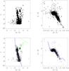 |
Fig. 3 Graphs for the filtering of open cluster NGC 2477. Upper graphs give all UBV data and lower ones the filtered and weighted data and the fitted isochrone and ZAMS (solid lines). The symbol size is proportional to likelihood value. |
 |
Fig. 4 Graphs for the filtering of open cluster NGC 2477. Upper graphs give all 2MASS data and lower ones the filtered and weighted data and the fitted isochrone and ZAMS (solid lines). The symbol size is proportional to likelihood value. |


 |
Fig. 9 Same as Fig. 1 for Berkeley 32. |
 |
Fig. 10 Same as Fig. 2 for Berkeley 32. |


 |
Fig. 21 Same as Fig. 1 for Melotte 105 (Ref. 289). |
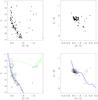 |
Fig. 22 Same as Fig. 1 for Melotte 105 (Ref. 32). |
 |
Fig. 23 Same as Fig. 2 for Melotte 105. |
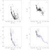 |
Fig. 24 Same as Fig. 1 for Trumpler 1 (Ref. 86). |
 |
Fig. 25 Same as Fig. 1 for Trumpler 1 (Ref. 320). |
 |
Fig. 26 Same as Fig. 2 for Trumpler 1. |


Information obtained from the version 3.1 of the New catalogue of optically visible open clusters and candidates (Dias et al. 2002), available electronically at www.astro.iag.usp.br/~wilton
Acknowledgments
The authors are grateful to an anonymous referee for very helpful suggestions. We acknowledge support from the Brazilian Institutions CNPq and INCT-A. H. Monteiro acknowledges the CNPq (Grant 470135/2010-7) and FAPEMIG (Grant APQ-02030-10). T. Caetano thanks the CNPq. This publication makes use of data products from the Two Micron All Sky Survey, which is a joint project of the University of Massachusetts and the Infrared Processing and Analysis Center/California Institute of Technology, funded by the National Aeronautics and Space Administration and the National Science Foundation. We employed catalogues from CDS/Simbad (Strasbourg) and
Digitized Sky Survey images from the Space Telescope Science Institute (US Government grant NAG W-2166). We also made use of the WEBDA open cluster database.
References
- Dias, W. S., & Lépine, J. R. D. 2005, ApJ, 629, 825 [NASA ADS] [CrossRef] [Google Scholar]
- Dias, W. S., Alessi, B. S., Moitinho, A., & Lépine, J. R. D. 2002, A&A, 389, 871 [NASA ADS] [CrossRef] [EDP Sciences] [Google Scholar]
- Dias, W. S., Assafin, M., Flório, V., Alessi, B. S., & Líbero, V. 2006, A&A, 446, 949 [NASA ADS] [CrossRef] [EDP Sciences] [Google Scholar]
- Lépine, J. R. D., Cruz, P., Scarano, S., Jr., et al. 2011, MNRAS, 417, 698 [NASA ADS] [CrossRef] [Google Scholar]
- Bica, E., Bonatto, C., & Dutra, C. M. 2004, A&A, 422, 555 [NASA ADS] [CrossRef] [EDP Sciences] [Google Scholar]
- Bonatto, C., & Bica, E. 2007, MNRAS, 377, 1301 [NASA ADS] [CrossRef] [Google Scholar]
- Bonatto, C., Bica, E., & Girardi, L. 2004, A&A, 415, 571 [NASA ADS] [CrossRef] [EDP Sciences] [Google Scholar]
- Carraro, G., & Costa, E. 2007, A&A, 464, 573 [NASA ADS] [CrossRef] [EDP Sciences] [Google Scholar]
- Carraro, G., Vázquez, R. A., Costa, E., et al. 2010, ApJ, 718, 683 [NASA ADS] [CrossRef] [Google Scholar]
- Clariá, J. J., & Lapasset, E. 1986, AJ, 91, 326 [NASA ADS] [CrossRef] [Google Scholar]
- Dutra, C. M., Santiago, B. X., & Bica, E. 2002, A&A, 381, 219 [NASA ADS] [CrossRef] [EDP Sciences] [Google Scholar]
- Girardi, L., Bressan, A., Bertelli, G., et al. 2000, A&AS, 141, 371 [NASA ADS] [CrossRef] [EDP Sciences] [Google Scholar]
- Girardi, L., Bertelli, G., Bressan, A., et al. 2002, A&A, 391, 195 [NASA ADS] [CrossRef] [EDP Sciences] [Google Scholar]
- Kronberger, M., Teutsch, P., Alessi, B., et al. 2006, A&A, 447, 921 [NASA ADS] [CrossRef] [EDP Sciences] [Google Scholar]
- Marigo, P., Girardi, L., Bressan, A., et al. 2008, A&A, 482, 883 [NASA ADS] [CrossRef] [EDP Sciences] [Google Scholar]
- Mermillioud, J.-C., & Paunzen, E. 2003, A&A, 410, 511 [NASA ADS] [CrossRef] [EDP Sciences] [Google Scholar]
- Monteiro, H., & Dias, W. S. 2011, A&A, 530, A91 [NASA ADS] [CrossRef] [EDP Sciences] [Google Scholar]
- Monteiro, H., Dias, W. S., & Caetano, T. C. 2010, A&A, 516, A2 [NASA ADS] [CrossRef] [EDP Sciences] [Google Scholar]
- Piatti, A. E., Clariá, J. J., & Ahumada, A. V. 2010, PASP, 122, 288 [NASA ADS] [CrossRef] [Google Scholar]
- Sánchez, N., Vicente, B., & Alfaro, E. J. 2010, A&A, 510, A78 [NASA ADS] [CrossRef] [EDP Sciences] [Google Scholar]
- Schlegel, D. J., Finkbeiner, D. P., & Davis, M. 1998, ApJ, 500, 525 [NASA ADS] [CrossRef] [Google Scholar]
- Soares, J. B., & Bica, E. 2002, A&A, 388, 172 [NASA ADS] [CrossRef] [EDP Sciences] [Google Scholar]
- Tadross, A. L. 2008, NewA, 13, 370 [Google Scholar]
- Tadross, A. L. 2011, JKAS, 44, 1 [Google Scholar]
- Vázquez, R. A., May, J., Carraro, G., et al. 2008, ApJ, 672, 930 [NASA ADS] [CrossRef] [Google Scholar]
- Vázquez, R. A., Moitinho, A., Carraro, G., & Dias, W. S. 2010, A&A, 511, A38 [NASA ADS] [CrossRef] [EDP Sciences] [Google Scholar]
All Tables
Basic parameters obtained for the investigated clusters with the new filter process and cross-entropy (CE) method.
All Figures
|
Fig. 1 Comparison of our fit results to those of Monteiro et al. (2010, Paper I). The error bars are obtained from the errors presented in Table 2 for the fits as explained in the text. The lines of 45o are the loci of equal values. |
| In the text | |
|
Fig. 2 Comparison of our fit results from applying the global optimization tool to fit isochrones to open clusters both with optical and 2MASS data using a weighted likelihood criterion. The error bars are presented in Table 2 for the fits as explained in the text. The lines of 45o are the loci of equal values. |
| In the text | |
|
Fig. 3 Graphs for the filtering of open cluster NGC 2477. Upper graphs give all UBV data and lower ones the filtered and weighted data and the fitted isochrone and ZAMS (solid lines). The symbol size is proportional to likelihood value. |
| In the text | |
|
Fig. 4 Graphs for the filtering of open cluster NGC 2477. Upper graphs give all 2MASS data and lower ones the filtered and weighted data and the fitted isochrone and ZAMS (solid lines). The symbol size is proportional to likelihood value. |
| In the text | |
|
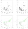
Fig. 9 Same as Fig. 1 for Berkeley 32. |
| In the text | |
|
Fig. 10 Same as Fig. 2 for Berkeley 32. |
| In the text | |
|
Fig. 21 Same as Fig. 1 for Melotte 105 (Ref. 289). |
| In the text | |
|
Fig. 22 Same as Fig. 1 for Melotte 105 (Ref. 32). |
| In the text | |
|
Fig. 23 Same as Fig. 2 for Melotte 105. |
| In the text | |
|
Fig. 24 Same as Fig. 1 for Trumpler 1 (Ref. 86). |
| In the text | |
|
Fig. 25 Same as Fig. 1 for Trumpler 1 (Ref. 320). |
| In the text | |
|
Fig. 26 Same as Fig. 2 for Trumpler 1. |
| In the text | |
 |
Fig. 29 Comparison of our fit with that of Bica et al. (2004) for Dias 6. See the text for details. |
| In the text | |
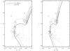 |
Fig. 30 Comparison of our fit with that of Tadross (2008) for Dias 6. See the text for details. |
| In the text | |
Current usage metrics show cumulative count of Article Views (full-text article views including HTML views, PDF and ePub downloads, according to the available data) and Abstracts Views on Vision4Press platform.
Data correspond to usage on the plateform after 2015. The current usage metrics is available 48-96 hours after online publication and is updated daily on week days.
Initial download of the metrics may take a while.