© ESO, 2012

1. Introduction

Many quantities in astronomy, physics, and other sciences are most naturally represented as functions on the unit sphere S². Typical examples in astrophysics are the celestial sphere or the surfaces of celestial bodies. A standard operation for such functions is to compute their integrals over the whole sphere or parts of it, usually with some weight functions, to express total sums, averages, moments, and so on. Integrals over any shape other than the sphere, but ones that can be mapped one-to-one onto S², are handled using the surface element (Jacobian) as a weight function and are thus reduced to exactly the same spherical problem.

Brightness integrals or lightcurves are an important example of these surface integrals. As shown in Ďurech & Kaasalainen (2003), virtually all lightcurves of single asteroids in realistic observing geometries can be explained, i.e., fitted down to noise level, by convex surfaces approximating the global shape of the target. Thus, for all photometric purposes, such targets can be represented as convex models. Convex models require no ray-tracing as their brightnesses can be expressed as integrals over a simply defined part of S². What is more, most models are very conveniently and compactly described by function series (based on spherical harmonics) in lightcurve inversion (Kaasalainen et al. 1992a; 2001; 2006). One can thus, in principle, compute their total brightness (especially that of models of real asteroids) at arbitrary viewing geometries without the polyhedral surface representations that are the standard means of integration in lightcurve simulation and inversion. In this paper, we show that function integration is faster and, in many ways, simpler than polyhedral modelling. This is particularly advantageous for large-scale simulations and inverse problems involving thousands of targets and the repeated computation of millions of lightcurve points.

A traditional way to compute surface integrals is to tessellate the surface, i.e., to represent it as a polyhedral approximation, usually with triangular facets of similar size (triangulation). The integral is then approximated as a sum over the facet areas multiplied by the corresponding values of the integrand functions. The approximation can be made arbitrarily accurate by making the triangulation mesh denser. However, in the (log N,log Δ)-plane, where Δ is the approximation error and N the number of facets, i.e., of function evaluations required, the accuracy log Δ(log N) improves only with a linear slope of  − 1. To reduce the error by a half, one must double the number of computations. This is the least efficient way of computing the integrals, equivalent to the elementary way of computing one-dimensional integrals as Riemann sum approximations by dividing the integration interval into equally large steps.

In the one-dimensional case of real-valued functions on R, or its Cartesian multidimensional version Rⁿ, the standard way of improving the computation is to use quadratures such as Gauss-Legendre (or Gauss-Chebyshev etc., depending on weight functions). For large n, the only computationally feasible way is to use Monte Carlo techniques. The sphere S² has a markedly different topology from R²; using Gaussian quadratures, some of the computations are wasted on integration points clustered too tightly around the two poles, and the integration scheme is thus manifestly dependent on the coordinate frame. Evidently, the most natural quadrature for S² is quite different from the Cartesian case.

Lebedev quadrature (Lebedev & Laikov 1999) is designed to be rather automatically optimal for smooth and continuous integrand functions over the whole of S², in the same sense that Gaussian quadrature is optimal for R. The Lebedev scheme combines the almost equidistant and rotationally invariant distribution of points on S² with the efficiency of quadratures (a low vertical positioning and a slope steeper than  − 1 for the log Δ(log N)-curve). However, it is not designed for integrals only over a part of S². For these, we need to consider and test various approaches to see which is the most useful one in practice. Our purpose is to find the optimal approach for accuracy levels corresponding to typical data noise.

This paper is organized as follows. In Sect. 2 we review the problem of the computing of lightcurve or brightness integrals on S², and discuss its numerical representation in the form of quadratures. In Sect. 3 we present efficiency results from various sample cases, and also note a particular formulation for integrals on triaxial ellipsoids. In Sect. 4 we describe the use and efficiency of the quadrature scheme in both inversion and simulations (e.g., Monte Carlo sampling). In the concluding Sect. 5 we sum up and discuss some aspects of the quadrature approach.

2. Brightness integrals as quadratures

A detailed discussion of the theoretical aspects of the problem of computing the total brightness of a convex surface is given in Kaasalainen et al. (1992a; 2001; 2006), so here we only review the main points and notations relevant to our search of the optimal method.

Let the illumination (subsolar) and viewing (sub-Earth) directions in a coordinate system fixed to the target body be denoted by ω₀,ω ∈ S². Here entities in S², defined by two direction angles, are identified with unit vectors in R³. Thus, e.g., the outward unit normal vector η ∈ S² is given by η = η(ϑ,ψ) (with ϑ measured from the pole); i.e., ${\mathit{\eta }}_{\mathrm{1}}\mathrm{=}\sin \mathit{\vartheta }\cos \mathit{\psi ,} {\mathit{\eta }}_{\mathrm{2}}\mathrm{=}\sin \mathit{\vartheta }\sin \mathit{\psi ,} {\mathit{\eta }}_{\mathrm{3}}\mathrm{=}\cos \mathit{\vartheta }\mathit{.}$(1)Denoting the portion of the surface both visible and illuminated by A ₊ , the total (integrated) brightness of the body is given by $\mathit{L}\mathrm{\left(}{\mathit{\omega }}_{\mathrm{0}}\mathit{,\omega }\mathrm{\right)}\mathrm{=}{\mathrm{\int }}_{{\mathit{A}}_{\mathrm{+}}}\mathit{S}\mathrm{\left(}\mathit{\mu ,}{\mathit{\mu }}_{\mathrm{0}}\mathit{,\alpha }\mathrm{\right)}\hspace{0.17em}\mathit{G}\mathrm{\left(}\mathit{\vartheta ,\psi }\mathrm{\right)}\hspace{0.17em}\mathrm{d}\mathit{\sigma ,}$(2)where $\mathrm{d}\mathit{\sigma }\mathrm{=}\sin \mathit{\vartheta }\hspace{0.17em}\mathrm{d}\mathit{\vartheta }\hspace{0.17em}\mathrm{d}\mathit{\psi ,}$(3)and the scattering function S(μ,μ₀,α) is taken to depend on the viewing geometry quantities $\mathit{\mu }\mathrm{=}\mathit{\omega }\mathrm{·}\mathit{\eta ,} {\mathit{\mu }}_{\mathrm{0}}\mathrm{=}{\mathit{\omega }}_{\mathrm{0}}\mathrm{·}\mathit{\eta ,} \cos \mathit{\alpha }\mathrm{=}{\mathit{\omega }}_{\mathrm{0}}\mathrm{·}\mathit{\omega }\mathit{.}$(4)Thus A ₊  includes those points on the surface for which μ₀,μ ≥ 0. The curvature function G ≥ 0 of the surface is $\mathit{G}\mathrm{\left(}\mathit{\vartheta ,\psi }\mathrm{\right)}\mathrm{=}\frac{\mathit{J}\mathrm{\left(}\mathit{\vartheta ,\psi }\mathrm{\right)}}{\sin \mathit{\vartheta }}\mathit{,}$(5)where J: = |J| is the norm of the Jacobian vector ${J}\mathrm{\left(}\mathit{\vartheta ,\psi }\mathrm{\right)}\mathrm{=}\frac{\mathit{\partial }{x}}{\mathit{\partial \vartheta }}\mathrm{\times }\frac{\mathit{\partial }{x}}{\mathit{\partial \psi }}\mathit{,}$(6)where x(ϑ,ψ) gives the surface as a function of the surface normal direction.

The standard choice, adopted in Kaasalainen et al. (2001), for the numerical computation of (2) is the tessellation of S² into N almost equal-sized facets approximating the surface as a polyhedron: $\mathit{L}\mathrm{\left(}{\mathit{\omega }}_{\mathrm{0}}\mathit{,\omega }\mathrm{\right)}\mathrm{\approx }\sum _{\mathit{j}\mathrm{=}\mathrm{1}}^{\mathit{N}}\mathit{S}\mathrm{\left(}{\mathit{\mu }}_{\mathrm{0}}^{\mathrm{\left(}\mathit{j}\mathrm{\right)}}\mathit{,}{\mathit{\mu }}^{\mathrm{\left(}\mathit{j}\mathrm{\right)}}\mathit{,\alpha }\mathrm{\right)}\hspace{0.17em}\mathit{G}\mathrm{\left(}{\mathit{\eta }}_{\mathit{j}}\mathrm{\right)}\hspace{0.17em}\mathrm{\Delta }{\mathit{\sigma }}_{\mathit{j}}\mathit{,}$(7)where η_j is the surface normal of the facet j, and the tessellation is done on S² with any standard scheme, with Δσ_j as the area of the facet j on S². Thus the area of the facet j on the actual surface is G(η_j)   Δσ_j, and this is solved for in the inverse problem, leading to surface reconstruction via the Minkowski procedure (Kaasalainen et al. 1992a; 2001).

Another, more analytical option for evaluating (2) is to use quadratures rather than the geometrically intuitive equal-facet tessellation. The main principle in any quadrature scheme is to choose the evaluation points of the integrand function (and their corresponding weights) in a cleverer way than a brute-force approximation of a Riemann sum. This choice is based on an assumption of the form of the function. Gaussian quadrature is based on the fact that any one-dimensional integral (with finite itegration limits) over any polynomial f(x) of (2N − 1)th degree can be evaluated exactly by choosing a set, independent of f and tabulated in one step, of merely N unevenly distributed evaluation points or abscissae x_i (to be scaled linearly according to the integration interval), and their weights w_i so that $\int \mathit{f}\mathrm{\left(}\mathit{x}\mathrm{\right)}\hspace{0.17em}\mathrm{d}\mathit{x}\mathrm{=}\sum _{\mathit{i}}\mathit{f}\mathrm{\left(}{\mathit{x}}_{\mathit{i}}\mathrm{\right)}\mathit{w}i$(8)(Arfken 1985), so the sum can be used as a good approximation of integrals over any other well-behaved functions f(x) (depending on the number of abscissae chosen). Consequently, any two-dimensional integral ${\mathrm{\int }}_{\mathit{a}}^{\mathit{b}}{\mathrm{\int }}_{\mathit{c}\mathrm{\left(}\mathit{v}\mathrm{\right)}}^{\mathit{d}\mathrm{\left(}\mathit{v}\mathrm{\right)}}\mathit{f}\mathrm{\left(}\mathit{u,v}\mathrm{\right)}\hspace{0.17em}\mathrm{d}\mathit{u}\hspace{0.17em}\mathrm{d}\mathit{v}$(9)over a double polynomial f(u,v) of degrees L,M in u,v can be evaluated by using (L + 1)(M + 1)/4 tabulated abscissae and their weights. Here we are interested in the spherical harmonics ${\mathit{Y}}_{\mathit{l}}^{\mathit{m}}\mathrm{\left(}\mathit{u,v}\mathrm{\right)}$ that can be expressed as double polynomials in u,v. Since the v-part is expressed by e^imv, i.e., two polynomials from the functions sinmv and cosmv, and we usually have M = L, the maximum degree of the spherical harmonics used, the number of abscissae needed for a Gaussian quadrature over spherical harmonics is (L + 1)²/2. The quadrature is usually a combination of Gauss-Legendre and Gauss-Chebyshev to account for the trigonometric functions with the corresponding weight function.

We now investigate the available options for writing Eq. (2) in a standard quadrature form. In Kaasalainen et al. (1992a), the analytical handling of Eq. (2), leading to the uniqueness proof for the inverse problem, required transforming the integrand into a coordinate system in which ω₀,ω are in the new xy-plane. This yields simple integration limits, but comes at the price of a more complicated integrand: $\mathit{L}\mathrm{\left(}{\mathit{\omega }}_{\mathrm{0}}\mathit{,\omega }\mathrm{\right)}\mathrm{=}{\mathrm{\int }}_{\mathit{\alpha }}^{\mathit{\pi }}{\mathrm{\int }}_{\mathrm{0}}^{\mathit{\pi }}{\mathit{P}}_{\mathrm{R}}\mathrm{\left(}{\mathit{\omega }}_{\mathrm{0}}\mathit{,\omega }\mathrm{\right)}\mathit{G}\mathrm{\left(}\mathit{\vartheta ,\psi }\mathrm{\right)}\mathit{S}\mathrm{\left(}\mathit{\mu ,}{\mathit{\mu }}_{\mathrm{0}}\mathit{,\alpha }\mathrm{\right)}\hspace{0.17em}\mathrm{d}\mathit{\sigma ,}$(10)where $\mathit{\mu }\mathrm{=}\sin \mathit{\psi }\sin \mathit{\vartheta ,} {\mathit{\mu }}_{\mathrm{0}}\mathrm{=}\sin \mathrm{(}\mathit{\psi }\mathrm{-}\mathit{\alpha }\mathrm{)}\sin \mathit{\vartheta ,}$(11)and the operator P_R(ω₀,ω) transforms a function into the new system obtained by the frame rotation matrix R(ω₀,ω). Thus, ${\mathit{P}}_{\mathrm{R}}\mathrm{\left(}{\mathit{\omega }}_{\mathrm{0}}\mathit{,\omega }\mathrm{\right)}\mathit{G}\mathrm{\left(}\mathit{\vartheta ,\psi }\mathrm{\right)}\mathrm{=}\mathit{G}\mathrm{\left(}{\mathrm{R}}^{-1}\mathrm{\right(}{\mathit{\omega }}_{\mathrm{0}}\mathit{,\omega }\mathrm{\left)}\mathit{\eta }\mathrm{\right(}\mathit{\vartheta ,\psi }\mathrm{\left)}\mathrm{\right)}\mathit{,}$(12)or, if G is of the form $\mathit{G}\mathrm{=}\mathit{G}\mathrm{\left(}\mathrm{\right\{}{\mathit{Y}}_{\mathit{l}}^{\mathit{m}}\mathrm{\left(}\mathit{\vartheta ,\psi }\mathrm{\right)}\mathrm{\left\}}\mathrm{\right)}$, where $\mathrm{\left\{}{\mathit{Y}}_{\mathit{l}}^{\mathit{m}}\mathrm{\right(}\mathit{\vartheta ,\psi }\mathrm{\left)}\mathrm{\right\}}$ denotes some set of spherical harmonics with a number of various degrees and orders l,m, ${\mathit{P}}_{\mathrm{R}}\mathrm{\left(}{\mathit{\omega }}_{\mathrm{0}}\mathit{,\omega }\mathrm{\right)}\mathit{G}\mathrm{\left(}\mathit{\vartheta ,\psi }\mathrm{\right)}\mathrm{=}\mathit{G}\left(\left\{\sum _{\mathit{i}\mathrm{=}\mathrm{-}\mathit{m}}^{\mathit{m}}{\mathit{r}}_{\mathit{i}}^{\mathit{lm}}\mathrm{\left(}{\mathit{\omega }}_{\mathrm{0}}\mathit{,\omega }\mathrm{\right)}{\mathit{Y}}_{\mathit{l}}^{\mathit{i}}\mathrm{\left(}\mathit{\vartheta ,\psi }\mathrm{\right)}\right\}\right)\mathit{,}$(13)where ${\mathit{r}}_{\mathit{i}}^{\mathit{lm}}\mathrm{\left(}{\mathit{\omega }}_{\mathrm{0}}\mathit{,\omega }\mathrm{\right)}$ are the so-called D-matrices of spherical harmonics (Kaasalainen et al. 1992a).

The integration limits of Eq. (10) nominally allow two-dimensional Gaussian quadrature, but the forms (12) and (13) both cause significant computational overhead, as well as complications in inverse problem applications. Using Eq. (12) calls for additional computations as the evaluation points of G(η) are redefined, and the transformation (13) introduces additional multiplications for function values at the evaluation points. Furthermore, the inverse problem solution typically requires the derivatives of L with respect to the rotation parameters of the target that define ω₀,ω, and this leads to complicated derivative chains in both (12) and (13) which increase the computational cost further. Note also that, due to the existence of S in the integrand, and the fact that we usually use functions $\exp \mathrm{\left(}{\mathit{Y}}_{\mathit{l}}^{\mathit{m}}\mathrm{\right)}$ to guarantee positivity, the nominal number of quadrature points discussed above is not sufficient for a series of degree L.

Still another way to do Gaussian quadrature over a part of S² is to keep the integrand simple but to write the integration limits as, e.g., $\mathit{L}\mathrm{=}{\mathrm{\int }}_{{\mathit{\psi }}_{\mathrm{1}}\mathrm{\left(}{\mathit{\omega }}_{\mathrm{0}}\mathit{,\omega }\mathrm{\right)}}^{{\mathit{\psi }}_{\mathrm{2}}\mathrm{\left(}{\mathit{\omega }}_{\mathrm{0}}\mathit{,\omega }\mathrm{\right)}}{\mathrm{\int }}_{{\mathit{\vartheta }}_{\mathrm{1}}\mathrm{\left(}\mathit{\psi }\mathrm{;}{\mathit{\omega }}_{\mathrm{0}}\mathit{,\omega }\mathrm{\right)}}^{{\mathit{\vartheta }}_{\mathrm{2}}\mathrm{\left(}\mathit{\psi }\mathrm{;}{\mathit{\omega }}_{\mathrm{0}}\mathit{,\omega }\mathrm{\right)}}\mathit{S}\mathrm{\left(}\mathit{\mu ,}{\mathit{\mu }}_{\mathrm{0}}\mathit{,\alpha }\mathrm{\right)}\hspace{0.17em}\mathit{G}\mathrm{\left(}\mathit{\vartheta ,\psi }\mathrm{\right)}\hspace{0.17em}\sin \mathit{\vartheta }\hspace{0.17em}\mathrm{d}\mathit{\vartheta }\hspace{0.17em}\mathrm{d}\mathit{\psi ,}$(14)but now the boundary equations μ = 0, μ₀ = 0 are implicit for both ψ_i and ϑ_i(ψ), so setting the Gaussian grid calls for computationally expensive root-finding, and the parameter derivatives are also somewhat cumbersome, as above.

Further overhead is caused in typical repeated lightcurve computations when the function G(η) cannot be evaluated at a set of fixed η_i in one step. This happens in the above integrals due to the changing viewing geometry that alters the integration limits, hence the sampling points of G(η) for each computation of L; for Eq. (10) this is caused by α(ω₀,ω) in the integration limits. If the number of lightcurve points for one target is M, that of computations required for evaluating S(μ,μ₀,α) is I, and K function evaluations are needed for determining G(η) (with, e.g., spherical harmonics), then the computational cost of fixed-G(η_i) evaluation grows as NMI, while that of Gaussian quadrature grows as NM(I + K), when N is the size of the η_i-grid. Since typically K ≫ I, the K/I-fold overhead is considerable.

In view of the above, we thus discard the use of the above forms for rendering (2) to a form suitable for Gaussian quadrature as the potentially reduced number of evaluation points, as compared to tessellation, is not nearly sufficient to compensate for the computational overhead in the applications in practice we have in mind. In these, the accuracy levels are around 1% (0.01 mag), where a few hundred facets suffice for tessellation computations in any case. In applications where high accuracy is needed, Gaussian quadrature over a part of S² via Eqs. (10) or (14) can be useful as the efficiency of any quadrature grows very fast with growing N when the integrand is smooth and continuous over the integration region.

Quadratures can also be introduced by formally writing the integral (2) over the whole of S² by introducing a transformation zeroeing S(μ,μ₀,α) in places: $\begin{array}{}\mathrm{˜}\\ \mathit{S}\end{array}\mathrm{\left(}\mathit{\mu ,}{\mathit{\mu }}_{\mathrm{0}}\mathit{,\alpha }\mathrm{\right)}\mathrm{=}\{\begin{array}{c}\\ \mathrm{0}\mathit{,}& \mathit{\mu }\mathrm{\le }\mathrm{0}\hspace{0.17em}\hspace{0.17em}\mathrm{or}\hspace{0.17em}\hspace{0.17em}{\mathit{\mu }}_{\mathrm{0}}\mathrm{\le }\mathrm{0}\\ \mathit{S}\mathrm{\left(}\mathit{\mu ,}{\mathit{\mu }}_{\mathrm{0}}\mathit{,\alpha }\mathrm{\right)}\mathit{,}& \mathrm{elsewhere}\mathit{,}\end{array}$(15)so that we have $\mathit{L}\mathrm{\left(}{\mathit{\omega }}_{\mathrm{0}}\mathit{,\omega }\mathrm{\right)}\mathrm{=}{\mathrm{\int }}_{\mathrm{0}}^{\mathrm{2}\mathit{\pi }}{\mathrm{\int }}_{\mathrm{0}}^{\mathit{\pi }}\mathit{G}\mathrm{\left(}\mathit{\vartheta ,\psi }\mathrm{\right)}\begin{array}{}\mathrm{˜}\\ \mathit{S}\end{array}\mathrm{\left(}\mathit{\mu ,}{\mathit{\mu }}_{\mathrm{0}}\mathit{,\alpha }\mathrm{\right)}\hspace{0.17em}\mathrm{d}\mathit{\sigma }\mathit{.}$(16)Now the integration limits are simple constants, so this can be readily computed with quadratures, and the evaluation points are the same for each viewing geometry. The only hitch is that the integrand is usually no longer smooth or not necessarily even continuous everywhere in the integration region (in contrast with polynomials), so it is not possible to give a simple estimate of the minimum size of the quadrature grid.

While we could use Gaussian quadrature to evaluate Eq. (16), Lebedev quadrature is a more natural choice. It is not based on the double-integral form, but instead evaluates integrals on the whole of S²; i.e., $\mathit{I}\mathrm{=}{\mathrm{\int }}_{\mathrm{0}}^{\mathrm{2}\mathit{\pi }}{\mathrm{\int }}_{\mathrm{0}}^{\mathit{\pi }}\mathit{f}\mathrm{\left(}\mathit{u,v}\mathrm{\right)}\sin \mathit{u}\hspace{0.17em}\mathrm{d}\mathit{u}\hspace{0.17em}\mathrm{d}\mathit{v}$(17)as an approximation 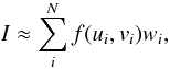$\mathit{I}\mathrm{\approx }\sum _{\mathit{i}}^{\mathit{N}}\mathit{f}\mathrm{\left(}{\mathit{u}}_{\mathit{i}}\mathit{,}{\mathit{v}}_{\mathit{i}}\mathrm{\right)}{\mathit{w}}_{\mathit{i}}\mathit{,}$(18)where the evaluation points (u_i,v_i) and their weights w_i can be tabulated for various N with standard algorithms (Lebedev & Laikov 1999). These tables can be called in the evaluations in the same way as with other quadratures. Software for creating the tables is available on the Internet¹, and sample tables and Matlab software are available from the authors.

For Lebedev quadrature, the number of required points in the grid is 2/3 of the Gaussian case, scaling approximately as (L + 1)²/3 when the integrand f is assumed to be a spherical harmonics series with maximum degree L so that the quadrature yields the exact value of the integral (Lebedev & Laikov 1999; Wang et al. 2003). Lebedev quadrature is also likely to give more accurate values than a Gaussian one in the case of a non-smooth integrand because of its almost even distribution of points on S² that also makes the computation virtually independent of the coordinate frame. This is depicted in Fig. 1; vertices are the Lebedev points, and the connecting edges are added by Delaunay triangulation to illustrate how the node distribution somewhat resembles that of typical tessellation.

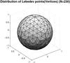Fig. 1 The distribution of Lebedev points on the unit sphere.

The derivation of the abscissae and weights is more complicated than in the Gaussian one-dimensional case due to the wholesale operation over S² that takes rotational symmetries into account. However, the tabulated end result is just as easy to use as in the one-dimensional Gaussian quadrature. Lebedev quadrature is essentially an advanced method for arranging evaluation points such that their distribution is approximately but not completely even, and consequently their weights w_i are not uniform (in contrast with standard tessellation that aims at similar Δσ). This predictive use of symmetry gives a competitive edge over both equal-facet tessellation and Gaussian quadrature. Most of the points have weights of roughly similar sizes, but the values of some weights are much smaller than the average and, depending on the chosen number of points, some weight values may even be negative.

In fact, for Lebedev schemes with positive weight values, Lebedev quadrature is formally equivalent to a customized tessellation scheme, the weights being interchangeable with the facet areas of a polyhedron. Here  ∑ _iw_i = 4π; by the construction of Lebedev quadrature, the polyhedron approximates the unit sphere. Even though no exact description of such an equivalence relation is needed for the problem here, we note that the locations of the vertices corresponding to the areas can be determined by, e.g., solving the polyhedral Minkowski problem (Kaasalainen et al. 2001; 2006). Figure 1 portrays a dual image of such a polyhedral tessellation, vertices corresponding to facets. Lebedev points are thus not directly the vertices of an optimal tessellation, but they indirectly define one for certain cases.

Now, with 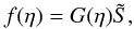$\mathit{f}\mathrm{\left(}\mathit{\eta }\mathrm{\right)}\mathrm{=}\mathit{G}\mathrm{\left(}\mathit{\eta }\mathrm{\right)}\begin{array}{}\mathrm{˜}\\ \mathit{S}\end{array}\mathit{,}$(19)many of the f(η_i) vanish, so we take the quadrature sum only over the points for which μ₀,μ > 0, just as in the tessellation sum.

To illustrate the remarkable power of Lebedev quadrature on the whole of S² for a smooth and continuous integrand, we consider the simple integral 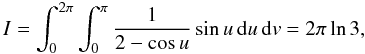$\mathit{I}\mathrm{=}{\mathrm{\int }}_{\mathrm{0}}^{\mathrm{2}\mathit{\pi }}{\mathrm{\int }}_{\mathrm{0}}^{\mathit{\pi }}\frac{\mathrm{1}}{\mathrm{2}\mathrm{-}\cos \mathit{u}}\sin \mathit{u}\hspace{0.17em}\mathrm{d}\mathit{u}\hspace{0.17em}\mathrm{d}\mathit{v}\mathrm{=}\mathrm{2}\mathit{\pi }\ln \mathrm{3}\mathit{,}$(20)and plot the curves log Δ(log N) of the relative error Δ of the numerical value (from comparison with the analytical one) in the (log N,log Δ)-plane in Fig. 2. The error of the triangulation sum is plotted with asterisks (with N for the number of facets), and that of the quadrature with circles; the saturation of the quadrature is due to machine accuracy. This curve also reflects the fact that quadratures over a well-behaved integrand always eventually win over equal-facet or standard tessellation (here we refer to this triangulation by the terms “tessellation” and “triangulation”) even if there is computational overhead, as discussed with Gaussian quadrature over a part of S² above.

We are now left with two methods to compare: the tessellation sum (7) and the Lebedev sum (18). Our hypothesis of the superior efficiency of using $\begin{array}{}{\mathrm{˜}}_{}\\ \mathit{S}\end{array}$ with Lebedev quadrature on S² rests on the assumption that the quadrature can handle the non-smooth behaviour of $\begin{array}{}{\mathrm{˜}}_{}\\ \mathit{S}\end{array}$ without invoking too many function evaluations; i.e., if we think in terms of an optimal tessellation via the Lebedev procedure, it should retain its superior properties even when shadowing is included. In the next section we show that this is indeed the case. Apparently the fact that most realistic scattering models contain the common factor μμ₀, thus making the scattering function S(μ,μ₀) vanish at the integration boundary, also helps to retain the accuracy in the quadrature since the integrand is then at least continuous on all of S².

3. Benchmark examples

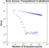Fig. 2 The error curves log Δ(log N) for computing the surface integral (20). Asterisks denote integration by triangulation, while circles are for integration by quadratures.

In this section, we present some benchmark tests of the accuracy of the methods of computing surface integrals as the size of the evaluation grids grows. In all figures, we have denoted the nominal number (N) of function evaluations in the tessellation and quadrature sums. In brightness examples, more than half of the evaluation points are skipped in the computation due to μ ≤ 0 or μ₀ ≤ 0 (i.e., $\begin{array}{}{}_{\mathrm{˜}}\\ \mathit{S}\end{array}\mathrm{=}\mathrm{0}$), but the relative portions of the skipped terms are the same for both sums, so the relative difference between the numbers of computations stays the same.

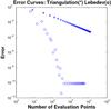Fig. 3 The error curves log Δ(log N) for computing the area of an ellipsoid. Asterisks denote integration by triangulation, while circles are for integration by quadratures.

As another example of Lebedev quadrature with smooth integrands over the whole of S², we plot in Fig. 3 the relative approximation error Δ of the area A of an ellipsoid against the size N of the evaluation grid (asterisks for tessellation facets and circles for Lebedev points; A is not analytically computable, but we use a numerical elliptic integral routine for establishing the accuracy). We thus compute 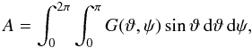$\mathit{A}\mathrm{=}{\mathrm{\int }}_{\mathrm{0}}^{\mathrm{2}\mathit{\pi }}{\mathrm{\int }}_{\mathrm{0}}^{\mathit{\pi }}\mathit{G}\mathrm{\left(}\mathit{\vartheta ,\psi }\mathrm{\right)}\sin \mathit{\vartheta }\hspace{0.17em}\mathrm{d}\mathit{\vartheta }\hspace{0.17em}\mathrm{d}\mathit{\psi ,}$(21)where G(ϑ,ψ) for an ellipsoid with semiaxes a,b,c is given in Kaasalainen et al. (1992b): 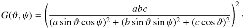$\mathit{G}\mathrm{\left(}\mathit{\vartheta ,\psi }\mathrm{\right)}\mathrm{=}{\left(\frac{\mathit{abc}}{\mathrm{(}\mathit{a}\sin \mathit{\vartheta }\cos \mathit{\psi }{\mathrm{)}}^{\mathrm{2}}\mathrm{+}\mathrm{(}\mathit{b}\sin \mathit{\vartheta }\sin \mathit{\psi }{\mathrm{)}}^{\mathrm{2}}\mathrm{+}\mathrm{(}\mathit{c}\cos \mathit{\vartheta }{\mathrm{)}}^{\mathrm{2}}}\right)}^{\mathrm{2}}\mathrm{·}$(22)Again, the quadrature is clearly superior to tessellation, as expected. The saturation at high accuracy is mostly due to numerical roundoff effects.

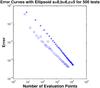Fig. 4 Average log Δ(log N) for geometrically scattering ellipsoids at various random observing geometries (asterisks for tessellation, circles for quadrature). N is the nominal number of evaluation points in a sum (over half of these are skipped).

The situation changes visibly when we consider the brightness of a geometrically scattering ellipsoid, i.e., S = μ. This can be computed analytically (Ostro & Connelly 1984) for comparison: $\mathit{L}\mathrm{=}\frac{\mathit{\pi }}{\mathrm{2}}\mathit{abc}\left[\sqrt{{\mathit{\omega }}^{\mathit{T}}\mathrm{M}\mathit{\omega }}\mathrm{+}\frac{{\mathit{\omega }}^{\mathit{T}}\mathrm{M}{\mathit{\omega }}_{\mathrm{0}}}{\sqrt{{\mathit{\omega }}_{\mathrm{0}}^{\mathit{T}}\mathrm{M}{\mathit{\omega }}_{\mathrm{0}}}}\right]\mathit{,}$(23)where $\mathrm{M}\mathrm{=}\left(\begin{array}{c}\\ \mathrm{1}\mathit{/}{\mathit{a}}^{\mathrm{2}}& \mathrm{0}& \mathrm{0}\\ \mathrm{0}& \mathrm{1}\mathit{/}{\mathit{b}}^{\mathrm{2}}& \mathrm{0}\\ \mathrm{0}& \mathrm{0}& \mathrm{1}\mathit{/}{\mathit{c}}^{\mathrm{2}}\end{array}\right)\mathit{.}$(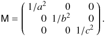24)We chose random realistic observing geometries with roughly the same proportions of terms skipped in the quadrature (facets omitted in the tessellation sum). Now the integrand function $\begin{array}{}{\mathrm{˜}}_{}\\ \mathit{S}\end{array}$ is not even continuous over S², and this shows in the quadrature error curve in Fig. 4 that is similar to the tessellation curve in its slope. However, it lies clearly below the latter, so even now its performance is noticeably better for our purposes. By changing the viewpoint 90 degrees and looking at the Δ(N)-curves as plots of the inverse function N(Δ) of the number of evaluations required for a given accuracy (especially around the relative error 0.01), one can clearly see the difference in computational cost between the two approaches.

Realistic scattering functions make $\begin{array}{}{\mathrm{˜}}_{}\\ \mathit{S}\end{array}$ continuous, which turns out to be of an important value. As a more general test, we examine the accuracy performance of Lebedev and tessellation grids by computing the brightness L at a number of random observing geometries for general convex shapes (asteroid models obtained from real lightcurve data). Now G(ϑ,ψ) is given by exponential spherical harmonics series of shape models as used in inversion (Kaasalainen et al. 2001). The scattering model used here was of the form combining the Lommel-Seeliger and Lambert laws, 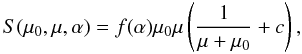$\mathit{S}\mathrm{\left(}{\mathit{\mu }}_{\mathrm{0}}\mathit{,\mu ,\alpha }\mathrm{\right)}\mathrm{=}\mathit{f}\mathrm{\left(}\mathit{\alpha }\mathrm{\right)}{\mathit{\mu }}_{\mathrm{0}}\mathit{\mu }\left(\frac{\mathrm{1}}{\mathit{\mu }\mathrm{+}{\mathit{\mu }}_{\mathrm{0}}}\mathrm{+}\mathit{c}\right)\mathit{,}$(25)which is typically used in lightcurve inversion; i.e., f(α) has no influence on the plot in Fig. 5. The reference value of L for computing Δ was obtained by applying a dense tessellation grid. Even though the performance of the quadrature is not as good as for actual integrals over the whole of S², the Lebedev-based scheme is clearly more efficient than tessellation also in that its error curve has a steeper slope. The same behaviour applies to, e.g., ellipsoids. Also, in Fig. 5, there are no scattered points such as the few seen in the Lebedev curve in Fig. 4. This is another beneficial effect of the continuity provided by the product μμ₀: when Lebedev points are sparse, a discontinuous integrand is more vulnerable to the geometry of the integration depending on whether individual Lebedev points (and their weights) are included in the quadrature sum or not. In general, predicting the performance of the quadrature-based approximation for discontinuous integrands, especially with a low number of evaluation points, is usually possible only by numerical tests.

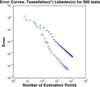Fig. 5 Average log Δ(log N) for general asteroid shapes and Lommel-Seeliger/Lambert scattering at various random observing geometries. N is the nominal number of evaluation points in a sum (over half of these are skipped).

The choice of the surface parametrization determines how the quadrature evaluation points are distributed, and for a priori known convex shapes we can, of course, use any representations of the surface points x(u,v), not necessarily just the Gaussian image x(η). In such cases we write $\mathit{L}\mathrm{\left(}{\mathit{\omega }}_{\mathrm{0}}\mathit{,\omega }\mathrm{\right)}\mathrm{=}{\mathrm{\int }}_{{\mathit{A}}_{\mathrm{+}}}\mathit{S}\mathrm{\left(}{\mathit{\mu }}_{\mathrm{0}}\mathit{,\mu ,\alpha }\mathrm{\right)}\hspace{0.17em}\mathit{J}\mathrm{\left(}\mathit{u,v}\mathrm{\right)}\hspace{0.17em}\mathrm{d}\mathit{u}\hspace{0.17em}\mathrm{d}\mathit{v,}$(26)and the normal vector required for determining μ,μ₀ is η = J/J. For example, ellipsoidal surfaces can be given in the standard parametrization ${\mathit{x}}_{\mathrm{1}}\mathrm{=}\mathit{a}\sin \mathit{u}\cos \mathit{v,} {\mathit{x}}_{\mathrm{2}}\mathrm{=}\mathit{b}\sin \mathit{u}\sin \mathit{v,} {\mathit{x}}_{\mathrm{3}}\mathrm{=}\mathit{c}\cos \mathit{u}\mathit{.}$(27)Thus, for an ellipsoid, we have, using u,v instead of ϑ,ψ in (6), $\frac{\mathit{J}\mathrm{\left(}\mathit{u,v}\mathrm{\right)}}{\sin \mathit{u}}\mathrm{=}\sqrt{\mathrm{(}\mathit{bc}\sin \mathit{u}\cos \mathit{v}{\mathrm{)}}^{\mathrm{2}}\mathrm{+}\mathrm{(}\mathit{ac}\sin \mathit{u}\sin \mathit{v}{\mathrm{)}}^{\mathrm{2}}\mathrm{+}\mathrm{(}\mathit{ab}\cos \mathit{u}{\mathrm{)}}^{\mathrm{2}}}\mathit{.}$(28)Since 0 ≤ u ≤ π and 0 ≤ v < 2π, the integral (26) is reduced to the standard Lebedev quadrature form with an integrand $\begin{array}{}{}_{\mathrm{˜}}\\ \mathit{S}\end{array}\mathit{J}\mathrm{\left(}\mathit{u,v}\mathrm{\right)}\mathit{/}\sin \mathit{u}$. As it happens, this parametrization is marginally but consistently more efficient than the Gaussian image, so combined with Lebedev quadrature, this is apparently the nominally fastest way to compute brightness integrals over ellipsoids. In practice, we found that the choice of surface parametrization has very little effect.

4. Efficiency in lightcurve simulation and inversion

We have shown above that, at an accuracy level of about 1% (corresponding to 0.01 mag in brightness), our scheme based on Lebedev quadrature is some five to ten times faster than triangulation, and orders of magnitude faster at higher accuracies. Thus, for direct brightness computations, i.e., lightcurve simulations, its efficiency is obvious. An important point is that functions are precomputed for chosen fixed points on S² just as with tessellation, so the procedure introduces no computational overhead. It is also easy to implement with Eqs. (18) and (19) using the known G(η) or J(u,v) of the shape and any chosen scattering model S. The increase in speed is particularly important for the massive lightcurve simulations typically needed for estimating the performance of large-scale sky surveys such as LSST, Pan-STARRS or Gaia. The simulations can be carried out with shapes (i.e., G(η)) known for real asteroids from lightcurve inversion (Ďurech et al. 2010). Simulations with ellipsoids are fastest to run using Eqs. (28) or (22).

In lightcurve inversion, most of the computation time is spent on evaluating lightcurves and the corresponding partial derivatives ∂L/∂P_i for the shape and rotation parameters P_i, so the enhanced speed in brightness computation yields an equally faster inversion procedure. The partial derivatives consume exactly the same computation time per evaluation point η_i for both quadrature and tessellation. From Eq. (18) we have $\frac{\mathit{\partial L}}{\mathit{\partial }{\mathit{P}}_{\mathrm{R}}}\mathrm{=}\sum _{\mathit{i}}{\mathit{w}}_{\mathit{i}}\mathit{G}\mathrm{\left(}{\mathit{\eta }}_{\mathit{i}}\mathrm{\right)}\frac{\mathit{\partial S}\mathrm{\left(}\mathit{\mu ,}{\mathit{\mu }}_{\mathrm{0}}\mathit{,\alpha }\mathrm{\right)}}{\mathit{\partial }{\mathit{P}}_{\mathrm{R}}}$(29)for rotation parameters P_R, and $\frac{\mathit{\partial L}}{\mathit{\partial }{\mathit{P}}_{\mathrm{S}}}\mathrm{=}\sum _{\mathit{i}}{\mathit{w}}_{\mathit{i}}\mathit{S}\mathrm{\left(}\mathit{\mu ,}{\mathit{\mu }}_{\mathrm{0}}\mathit{,\alpha }\mathrm{\right)}\frac{\mathit{\partial G}\mathrm{\left(}{\mathit{\eta }}_{\mathit{i}}\mathrm{\right)}}{\mathit{\partial }{\mathit{P}}_{\mathrm{S}}}$(30)for shape parameters P_S; the derivatives are of the same form as in the tessellation case (7). As before, functions (such as spherical harmonics) used in computing G(η) are precomputed for chosen fixed points on S² just as with tessellation. Lebedev quadrature is thus easy to substitute for tessellation in the inversion procedure, and it introduces no computational overhead, so the difference in the computational cost between the two approaches can be read directly from the Δ(N) (or N(Δ))-curves in Fig. 5. We plan to include a Lebedev-based inversion version of the convexinv procedure downloadable in the software section of the DAMIT website (Ďurech et al. 2010).

The simplest way to utilize the superior speed of the quadrature approach in lightcurve inversion is the “black box” mode where the optimized G(η) is used as an auxiliary unseen quantity, and the output parameters are those of rotation (pole direction and period). This is very useful in applications such as i) searching for the correct period in sparse photometric datasets from sky surveys when no period is evident a priori and a wide period range must be combed through (Kaasalainen 2004; Ďurech et al. 2006; 2007); ii) Monte-Carlo sampling to estimate the goodness-of-fit levels of the rotation parameters and thus their likelihood distributions; or iii) searching for and then fixing the pole and period prior to producing a high-resolution version of the shape as is usually done in the convex inversion procedure (Kaasalainen et al. 2001). Upon computing sample lightcurve inversion cases for targets previously analysed with tessellation, and using a reduced number of Lebedev evaluation points in accordance with Fig. 5, we found that the shape results were virtually indistinguishable from the previous ones, and the spin state parameters were essentially the same (e.g., typically within one or two degrees of the previous pole solution), i.e., well within uncertainty limits and amounting to a slightly different initial guess. We emphasize that the quadrature approach has very simple computational plug-in properties because it has exactly the same form as, and is thus directly interchangable with, the tessellation part in the software, producing essentially the same results faster.

Once the inversion procedure has provided the curvature function G (in, e.g., the form of the coefficients of a spherical harmonics series), this can be discretized into facet areas and normals usable by the Minkowski procedure by tessellation at the desired level of resolution, and this renders the result as a standard polyhedral model (Kaasalainen et al. 1992a; 2001). Another way to use the Lebedev-based approach is to solve for the separate values G(η_i) at Lebedev points η_i directly, in the same way that individual facet areas can be solved for in the tessellation-based inversion (using the exponential form G(η_i) = exp [ a_i]  to guarantee positivity). Once these values are obtained, the facet areas and normals required by the Minkowski procedure can be defined by G(η_i)w_i (when all w_i are positive) or by, e.g., using the Delaunay triangulation of the unit sphere shown in Fig. 1. The normals of the triangles give the facet normals of the final polyhedral model, and its facet areas are given by , where is the average value of G at the three vertices of the corresponding Delaunay triangle, and Δσ is the area of the triangle. Thus the quadrature approach provides exactly the same low/high-resolution options as the standard tessellation-based procedure (e.g., convexinv) of Kaasalainen et al. (1992a; 2001).

As described in Kaasalainen et al. (2001), the convex-shape procedure requires a regularization function (though usually with a very modest weight) to make sure that the resulting shape really is convex. This regularization is based on the three equations fulfilled by convex surfaces: ${\mathrm{\int }}_{\mathrm{0}}^{\mathrm{2}\mathit{\pi }}{\mathrm{\int }}_{\mathrm{0}}^{\mathit{\pi }}\mathit{G}\mathrm{\left(}\mathit{\vartheta ,\psi }\mathrm{\right)}{\mathit{\eta }}_{\mathit{i}}\mathrm{\left(}\mathit{\theta ,\psi }\mathrm{\right)}\sin \mathit{\vartheta }\hspace{0.17em}\mathrm{d}\mathit{\vartheta }\hspace{0.17em}\mathrm{d}\mathit{\psi }\mathrm{=}\mathrm{0}\mathit{,} \mathit{i}\mathrm{=}\mathrm{1}\mathit{,}\mathrm{2}\mathit{,}\mathrm{3}\mathrm{;}$(31)i.e., a proper curvature function G has no first-degree terms ${\mathit{Y}}_{\mathrm{1}}^{\mathit{m}}$ in its representation as a spherical harmonics series. In regularization, the left-hand sides are enforced to be as close to zero as possible. The regularization integral is directly in the Lebedev form, so it is conveniently computed with the same quadrature as the lightcurve integral.

5. Conclusions and discussion

This paper complements the study of the numerical computation of lightcurve integrals introduced and discussed in Kaasalainen et al. (1992a; 2001). We have systematically investigated and compared different methods of computing lightcurve-type integrals over varying integration regions on the unit sphere S². For smooth and continuous integrals over the whole of S², Lebedev quadrature is usually the optimal method, but integrals over a part of S² depend on the case. For these integrals, the usual choice of (Gaussian) quadrature is computationally expensive with lightcurves because then i) either the integration limits are complicated or they can be transformed into simpler ones only at the price of complicating the computation of the integrand; and ii) when lightcurve computations are repeated for an object, functions have to be constantly re-evaluated, whereas for tessellation and for quadrature over the whole of S² they can be evaluated in one step. For lightcurve integrals, and other integrals of similar nature, a modification of Lebedev quadrature by zeroeing a part of the quadrature sum outperforms both tessellation and quadrature over a part of S² (the latter when the required relative accuracy is not extraordinarily high – all realistic applications fall into this category). The scattering function usually vanishes at the integration boundary, which increases the efficiency of the computation as it makes the nominal integrand continuous.

Our scheme based on Lebedev quadrature is thus the optimal method for computating lightcurve integrals in practice. As a rule, Lebedev quadrature is five to ten times faster than triangulation at the accuracy level of 1% (0.01 mag), and it is orders of magnitude faster at accuracies of 0.1% and beyond (the slope of the accuracy curve is close to  − 2 rather than  − 1). The superior speed of the Lebedev approach is advantageous in

any applications in lightcurve inversion and simulation, and it is particularly suited to the automatic en masse analysis of thousands of targets from large-scale surveys, such as Pan-STARRS or LSST, or for simulations requiring the computation of a large number of lightcurve points.

Our method is very easy to substitute for tessellation in lightcurve simulation and inversion software since it is exactly similar to tessellation in its computational form: it merely uses fewer function evaluation points. The only thing that changes is that Lebedev weights (constants) are substituted for the fixed areas of facets on the unit sphere used in tessellation-based computations, and Lebedev points on the sphere are substituted for the fixed directions of the facet unit normals.

Acknowledgments

This work was supported by the Academy of Finland project “Modelling and applications of stochastic and regular surfaces in inverse problems”. The work of X. Lu is partially supported by grant No. 019/2010/A2 from the Science and Technology Development Fund, MSAR. We thank an anonymous referee for valuable comments and suggestions.

References

All Figures

	Fig. 1 The distribution of Lebedev points on the unit sphere.
In the text

	Fig. 2 The error curves log Δ(log N) for computing the surface integral (20). Asterisks denote integration by triangulation, while circles are for integration by quadratures.
In the text

	Fig. 3 The error curves log Δ(log N) for computing the area of an ellipsoid. Asterisks denote integration by triangulation, while circles are for integration by quadratures.
In the text

	Fig. 4 Average log Δ(log N) for geometrically scattering ellipsoids at various random observing geometries (asterisks for tessellation, circles for quadrature). N is the nominal number of evaluation points in a sum (over half of these are skipped).
In the text

	Fig. 5 Average log Δ(log N) for general asteroid shapes and Lommel-Seeliger/Lambert scattering at various random observing geometries. N is the nominal number of evaluation points in a sum (over half of these are skipped).
In the text

References

- Arfken, G. 1985, Mathematical methods for physicists, Academic, San Diego [Google Scholar]
- Ďurech, J., & Kaasalainen, M. 2003, A&A, 404, 709 [NASA ADS] [CrossRef] [EDP Sciences] [Google Scholar]
- Ďurech, J., Grav, T., Jedicke, R., et al. 2005, Earth Moon Planets, 97, 179 [Google Scholar]
- Ďurech, J., Scheirich, P., Kaasalainen, M., et al. 2007, Proc. IAU Symp. 236, ed. A. Milani, G. Valsecchi, & D. Vokrouhlicky, 191 [Google Scholar]
- Ďurech, J., Sidorin, V., & Kaasalainen, M. 2010, A&A, 513, A46 [NASA ADS] [CrossRef] [EDP Sciences] [Google Scholar]
- Kaasalainen, M. 2004, A&A, 422, L39 [NASA ADS] [CrossRef] [EDP Sciences] [Google Scholar]
- Kaasalainen, M., & Torppa, J. 2001, Icarus, 153, 24 [NASA ADS] [CrossRef] [Google Scholar]
- Kaasalainen, M., & Lamberg, L. 2006, Inverse Problems, 22, 749 [Google Scholar]
- Kaasalainen, M., Lamberg, L., Lumme, K., & Bowell, E. 1992a, A&A, 259, 318 [NASA ADS] [Google Scholar]
- Kaasalainen, M., Lamberg, L., & Lumme, K., 1992b, A&A, 259, 333 [NASA ADS] [Google Scholar]
- Lebedev, V., & Laikov, D. 1999, Doklady Math., 59, 477 [Google Scholar]
- Ostro, S., & Connelly, D. 1984, Icarus, 57, 443 [NASA ADS] [CrossRef] [Google Scholar]
- Wang, X., & Carrington, T. 2003, J. Theor. Comp. Chemistry, 2, 599 [CrossRef] [Google Scholar]