| Issue |
A&A
Volume 539, March 2012
|
|
|---|---|---|
| Article Number | L5 | |
| Number of page(s) | 4 | |
| Section | Letters | |
| DOI | https://doi.org/10.1051/0004-6361/201117930 | |
| Published online | 24 February 2012 | |
Detecting cosmic structure via 21-cm intensity mapping on the Australian Telescope Compact Array
1 Department of Astronomy & Astrophysics, University of Toronto, 50 St. George Street, Toronto, Ontario, M5S 3H4 n Canada
e-mail: This email address is being protected from spambots. You need JavaScript enabled to view it.
; This email address is being protected from spambots. You need JavaScript enabled to view it.
2 Canadian Institute of Theoretical Astrophysics, University of Toronto, 60 St. George Street, Toronto, Ontario, M5S 1A7, Canada
Received: 22 August 2011
Accepted: 5 February 2012
Abstract
The studies of the nature of dark energy have defined contemporary astrophysics. We report the first detection of a cosmic power spectrum using the Australian Telescope Compact Array interferometer in the 21-cm L-band. We obtained the power spectrum through cross-correlation with optical galaxies, as well as auto-correlation using radio data alone.
Key words: diffuse radiation / large-scale structure of Universe / galaxies: statistics / radio lines: galaxies / techniques: interferometric
© ESO, 2012
1. Introduction
One of the most puzzling discoveries in astronomy is the accumulating evidence that most of the content of the Universe is in the form of dark energy (DE). The most direct way to study DE, its properties and dynamics, is to use large-scale structure surveys. Mapping the intensity distribution of the sky in radio frequencies via the Stokes I parameter intensity mapping (IM) (Chang et al. 2008) is an efficient method for surveying large-scale structures (LSS), because it has the potential to quickly scan large volumes of the Universe and produce three-dimensional maps of matter density fields. Because it targets LSS, IM does not require resolving individual galaxies: the aggregate emission of many galaxies is sufficient.
A key feature for studying DE is the presence of baryon acoustic oscillations (BAO) in LSS. The BAO provide a co-moving “standard ruler” – the size of the cosmic sound horizon – which can be used to measure distances in an expanding Universe. Measuring the contribution of the different harmonics of BAO at different redshifts via the power spectrum of the matter distribution allows the precise determination of the expansion dynamics of the Universe. In particular, determining the kinematics of the expansion during the transition from a matter-dominated to a DE-dominated Universe – occurring at z < 2 – provides great insight into DE dynamics. Also, BAO structures smaller than ~10 Mpc (or about 20′ at z ~ 1) (Seo et al. 2008) do not need to be resolved: they are washed out by effects of non-linear growth of density perturbations.
Because hydrogen is the most abundant element in the Universe, its 21-cm transition line is the best tracer of LSS such as BAO. Redshifted 21-cm radiation will be a key signal in future large-scale structure and DE surveys (Wyithe & Loeb 2008), as well as in cosmological-tomography (Mao et al. 2008). In addition, IM using the 21-cm transition line is more appealing than previously used galaxy redshift surveys because it preserves information on a wider range of spatial scales. It is also an isolated transition, implying a one-to-one correspondence between frequency and redshift. Thus, minimal computational power is needed for spectral fitting. When extracting the 21-cm signal, the difficulty encountered is that its strength is a few orders of magnitude weaker than foreground emissions. Detection of the signal was proven possible using a single-dish telescope (Pen et al. 2009) and cross-correlating radio-frequency data with a galaxy redshift survey. We report here that 21-cm signal detection can also be obtained with an interferometer array, the Australian Telescope Compact Array (ATCA). Since the instrumental noise present due to imperfections in the detection system of an antennae is uncorrelated with that of another antenna, an interferometric array can be better calibrated than a single-dish telescope, such as the one used in the study by Pen et al. (2009). Therefore we were able to achieve enough sensitivity to suggest that the cosmic signal from galactic surveys is consistent with the auto-correlation signal using only radio-frequency data.
The goal of the present work is not to detect BAO, since our redshift and angular coverage prohibits this, but rather to report a feasibility study that uses IM using radio interferometers to detect the power spectrum using signal coming from galaxies and galaxy clusters. Future surveys of LSS can use this method to efficiently detect BAO and derive constraints on DE dynamics.
2. Data
ATCA is a six-antennae interferometer; each antenna is 22 m. ATCA’s compact H75 configuration is ideal for IM. In this configuration, three antennae are along the east-west track and two are along the north-south track, so that antennae 1 through 5 have baselines less than 100 m. Antenna 6 is stationary and is aligned along the east-west direction about 4.4 km away from the array centre. Because it is stationary, antenna 6 was used to obtain the correct resolution in the images to study the smallest cosmological scales of the survey. Therefore, most of the data taken in the IM mode uses antenna 1 through 5. When antenna 6 was used, correlations of antennae 1–5 among themselves were not used. Hence, two types of maps were made, one with the cluster of antennae 1–5 and another using correlations between antenna 6 and 1 through 5. Correlations solely with antenna 6 were considered when re-binning the data to the smallest scale. Since there are missing baselines between the cluster of antennae 1–5 and antenna 6, correlations with antenna 6 were only used to set a bound on observations. Table 1 provides details on the baseline lengths for the antenna configuration with which data were gathered.
ATCA H75 configuration baseline lengths in meters.
Using ATCA’s L-Band feed, Chandra’s Deep Field South (CDFS) region was chosen for data collection. This region is far away from the synchrotron emission from the galactic disk. Only little continuum emission is present. The area surveyed was 0.56 × 0.56 degrees centered at (3h32m28s, − 27°48′30′′) (J2000). ATCA sensitivities, obtained from the Australia Telescope National Facility (ATNF) website1, are presented in Table 2.
ATCA H75 sensitivities and specifications.
The bandwidth calibrated in this study spans from 1.135 GHz to 1.647 GHz, for a total of 512 MHz with a channel width of 1 MHz. This is significantly more bandwidth than was used in the previous study by Pen et al. (2009), where only 64 MHz of total bandwidth was available. Our redshift coverage of 21-cm radiation ranges up to z = 0.25.
The primary flux and bandpass calibrator is PKSB1934-638 with a flux of 14.95 Jy. After observing the flux calibrator for 15 min, data were acquired by alternating between CDFS regions, observed for 30 min at a time, and the phase calibrator PKSB0237-233, observed for 3 min at a time. The phase calibrator has a flux of 6.19 Jy. During our observations ATCA used all four linear polarizations, and recorded the full bandwidth of 2048 channels, available with the recently installed Compact Array Broadband Backend (CABB). Because the L-band receiver’s bandwidth is less than the bandwidth of CABB’s wide bands, only about 500 channels can effectively be used for 20 cm observations.
The observation run on the CDFS region lasted 26 h. The details on the observation runs are provided in Table 3.
Details regarding observation runs.
Data calibration was performed with MIRIAD, kindly provided by the Australia Telescope National Facility (ATNF). For both types of maps, once the data were calibrated, strong point sources were removed by making clean maps of the sky using uniform weighting (robustness = –2) in 2 MHz spectral chunks and subtracting these clean maps from the raw data. The procedure was stopped before the confusion noise became significant. Diffuse synchrotron-like emission remains present in our data. We assume the latter to be smooth with temperature T ~ να. The synchrotron-like signal was removed in the frequency domain via spectral subtraction, i.e. by subtracting the average of the nearest neighbors from the ith frequency bin. Then we used the singular value decomposition (SVD) which was performed as described by Chang et al. (2010), or by computing the eigenvalues of a matrix whose rows are sky coordinates and whose columns are frequency bins. After the SVD, a segregation of eigenvalues was observed with a significant gap between the groups. The segregation occurs because the synchrotron-like radiation is much brighter than the HI signal. The group composed of the highest eigenvalues should be removed because they correspond to unwanted signal. One way of doing this is via spectral subtraction. Spectral subtraction was performed until the highest eigenvalues of the SVD were removed. The described approach yielded sources with flux of about 0.06 mJy or less in the L-band, which is where Muxlow et al. (2005) found that starburst galaxies tend to occur typically. The SVD also allowed us to check the T ~ να power law behavior in frequency. The second way of eliminating the unwanted continuum emission is by removing the highest eigenvalues directly, as in Chang et al. (2010). By comparing direct removal and spectral subtraction, we found that the difference in signals obtained was not statistically significant.
3. Results and discussion
To evaluate the correlation function, only coarse-grained sky images were used. These images are difficult to interpret. Therefore, before we present them, we show in Fig. 1 two more informative images: a reference image using all available antennae in the ATCA H75 configuration and a high-resolution image, obtained using only correlations with antenna 6. In both cases, images of the stokes I parameter were obtained using the Miriad invert routine with robust weighting closer to natural weighting (robustness = 2) to increase the resolution as much as possible, such that strong point sources can be seen by eye; the entire frequency information is present in the map. The high-resolution image clearly shows the strongest point sources.
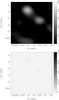 |
Fig. 1 Top: image obtained using all six antennae; bottom: correlations with antenna 6 only. The color wedges are in Jy. |
Twenty-six hours of integration time, self-calibration, and the CABB, a newly installed hardware, gave us enough data to remove unwanted signals from our maps down to a threshold of 0.020 mJy. After subtractions, the mean flux in the images was 0.038 mJy, and the root mean square variations were 0.020 mJy. To calculate correlation functions, the size of the grid cells in the radio images were varied. A coarse-grained grid had more flux per cell, because more astronomical sources are contributing than in a fine-grained grid. Changing the size of the grid effectively changes the scale to which the correlation function is sensitive. Figure 2 shows an image of the sky re-binned to 5 × 5 (0.112° × 0.112° per pixel) pixels before and after point sources and continuum emission were subtracted. The color wedge of the bottom panel of Fig. 2 was rescaled according to y = 0.400x + 0.038, where y is in mJy and x can be red off the color wedge, with the zero value corresponding to 0.038 mJy.
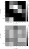 |
Fig. 2 Top: the field before subtraction of point sources and continuum emission with the color wedge in Jy; bottom: after subtraction of point sources and continuum emission with the color wedge, as expained in the text. |
Because we aim to detect cosmic structure solely via collective emissions of galaxies, two correlation functions were calculated: an auto-correlation that determines the power spectrum by correlating radio data to itself, and a cross-correlation function that correlates galaxy counts with radio fluxes. The auto-correlation function had its noise floor subtracted from the signal. Since the field of view is small, most of the contribution to the correlation function comes from the spectral (redshift) direction. The probed scales varied from 8 Mpc h-1 to 80 Mpc h-1. The size of the pixels was greater than the FWHM of the beam for the four largest scales, reaching the full size of the field of view in the transverse direction. The pixel-to-pixel correlations were small and washed out by the re-binning. Resolving the smallest scale required baselines of about 200 m. To achieve this resolution, the map produced via correlations with antenna 6 only was re-binned to the appropriate scale. The pixel-to-pixel correlations are present on the smallest scale (8 Mpc h-1) and the correlation data point on this scale is only a bound. The correlation functions and error bars were calculated as described by Chang et al. (2010), with slight variations for the cross-correlation. A 3D cube containing all the galactic positions for z ≤ 0.25 was constructed according to Chang et al. (2010) with the additional complexity that the Gaussian in the transverse plane had a FWHM that varied according to the number of antennae that were used in constructing the map. In the longitudinal direction of the 3D matrix, a Gaussian with a pairwise velocity dispersion of 500 km s-1 (Tinker et al. 2007) was used. That matrix was then re-binned to the probed cosmological scale.
The CDFS region was surveyed optically with the Very Large Telescope (VLT) VIsible Multi-Object Spectrograph (VIMOS) camera (Le Fèvre et al. 2003). The VLT’s CDFS galaxy survey by Balestra et al. (2010) contains a total of 5052 spectra and covers an area of 0.19 square degrees. Using only sources within z ≤ 0.25 overlapping with our ATCA’s CDFS region, we cross-correlated the radio to the VIMOS galaxy survey. The obtained correlation function is presented in Fig. 3. As noted by Pen et al. (2009), theoretical and experimental curves are assumed to obey a power law of the form ξ(r) = A(r/r0) − γ, where A is the average sky brightness for cross-correlations (Pen et al. 2009), r is the separation, and ξ is the correlation measured in Kelvin. Both theoretical curves assume r0 = 5.5 Mpc h-1 and γ = 1.8.
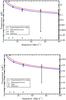 |
Fig. 3 Top graph illustrates the cross-correlation function while the bottom one depicts the auto-correlation function. Both the theoretical curves and the experimental cures follow a power law ξ(r) = A(r/r0) − γ. The error bars are 2σ bootstrap errors generated using 500 randomizations. The values provided at 8 Mpc h-1 are only upper bounds. |
The error bars for the auto- and cross-correlation were estimated using bootstrap analysis as described by Chang et al. (2010). Variances in correlation values are similar with 500 random samplings. The null tests, where one of the two data sets is randomized, were passed for both auto- and cross-correlation functions.
To the best of our knowledge, this is the first time that the cross-correlation function is computed using the IM technique on a radio interferometer. The detection of the cross-correlation function was reported before by Chang et al. (2010) and Pen et al. (2009) using the single-dish Green Bank and ATNF’s Parkes telescopes. Figure 3 also illustrates our detection of the cosmic structure using the auto-correlation function, where a power law curve is once again used as reference (Pen et al. 2009). The power law curve was fitted for both the auto and the cross-correlation functions using the curve fitting tool in MATLAB. Correlation functions obtained by using a Galactic surveys predict that γ is greater ~1.5 and r0 is greater ~2 Mpc h-1 (Meneux et al. 2006; Longair 2008), with typical values of ~1.8 and ~5.5 Mpc h-1, respectively (Pen et al. 2009). The cross-correlation function yields γ = 1.71 ± 0.49 and r0 = 3.52 ± 1.42 Mpc h-1 using a 95% confidence level (CL), whereas the auto-correlation gives γ = 1.65 ± 0.51 and r0 = 3.56 ± 1.53 Mpc h-1 (using a 95% CL). Both are consistent with galactic surveys. In calculating these fits, the data points on the lowest scale were omitted since it is only a bound.
A good indication of consistency with galactic surveys of cosmic structure in the auto-correlation function can be seen. This is a noteworthy result because it implies that current generation telescopes have enough sensitivity to map out the large-scale structure of the Universe using IM. Nevertheless, for IM to be truly exploited to its full potential – namely to detect BAO
in 21-cm emission – a telescope with more collecting area is needed, because it would allow for a significant portion of the sky to be mapped quickly and efficiently. This seems to be only possible with a dedicated survey telescope designed to have a large collecting area and a coarse grained resolution, such as the one proposed by Chang et al. (2008).
4. Conclusion
Using ATCA’s L-band in a compact H75 configuration, we have demonstrated that detecting the cosmic power spectrum can be possible – provided a sufficiently long integration time – with the aid of an optical galaxy survey such as that conducted by Balestra et al. (2010), which uses the VLT VIMOS camera. But, more importantly, the auto-correlation function shows that an optical survey is not necessary and that a radio telescope may be used alone to investigate the power spectrum using coarse resolution. Therefore, using ATCA, we demonstrated that the IM method has the ability to detect cosmic structure. Future investigations using this method with an extended volume, or sky coverage, should be even more efficient in detecting BAO and should consequently provide an avenue for new insight in dark energy (DE) studies. Finally, this approach eliminates the need for next-generation detector technology to perform such investigations: building a dedicated survey should provide sufficient sky coverage and sensitivity to effectively study DE dynamics.
Acknowledgments
This work was supported in part by the Natural Sciences and Engineering Research Council of Canada, and in part by the Fonds Québécois de la Recherche sur la Nature et les Technologies scholarships to G. Vujanovic. We kindly thank Angel Lopez-Sanchez for his support during data requisition and guidance pertaining to the operation of the telescope. We would also like to acknowledge Lister Staveley-Smith for assistance during the early stages of this project.
References
- Balestra, I., Mainieri, V., Popesso, P., et al. 2010, A&A, 512, A12 [NASA ADS] [CrossRef] [EDP Sciences] [Google Scholar]
- Chang, T.-C., Pen, U.-L., Peterson, J. B., & McDonald, P. 2008, Phys. Rev. Lett., 100, 091303 [NASA ADS] [CrossRef] [PubMed] [Google Scholar]
- Chang, T.-C., Pen, U.-L., Bandura, K., & Peterson, J. B. 2010, Nature, 466, 463 [NASA ADS] [CrossRef] [Google Scholar]
- Le Fèvre, O., Saisse, M., Mancini, D., et al. 2003, SPIE Conf. Ser., 4841, 1670 [Google Scholar]
- Longair, M. S. 2008, Galaxy Formation, 2nd edn. (Berlin: Springer) [Google Scholar]
- Mao, Y., Tegmark, M., McQuinn, M., Zaldarriaga, M., & Zahn, O. 2008, Phys. Rev. D, 78, 023529 [NASA ADS] [CrossRef] [Google Scholar]
- Meneux, B., Le Fèvre, O., Guzzo, L., et al. 2006, A&A, 452, 387 [NASA ADS] [CrossRef] [EDP Sciences] [Google Scholar]
- Muxlow, T. W. B., Richards, A. M. S., Garrington, S. T., et al. 2005, MNRAS, 358, 1159 [NASA ADS] [CrossRef] [Google Scholar]
- Pen, U.-L., Staveley-Smith, L., Peterson, J. B., & Chang, T.-C. 2009, MNRAS, 394, L6 [NASA ADS] [Google Scholar]
- Seo, H.-J., Siegel, E. R., Eisenstein, D. J., & White, M. 2008, ApJ, 686, 13 [NASA ADS] [CrossRef] [Google Scholar]
- Tinker, J. L., Norberg, P., Weinberg, D. H., & Warren, M. S. 2007, ApJ, 659, 877 [NASA ADS] [CrossRef] [Google Scholar]
- Wyithe, J. S. B., & Loeb, A. 2008, MNRAS, 383, 606 [NASA ADS] [Google Scholar]
All Tables
All Figures
|
Fig. 1 Top: image obtained using all six antennae; bottom: correlations with antenna 6 only. The color wedges are in Jy. |
| In the text | |
|
Fig. 2 Top: the field before subtraction of point sources and continuum emission with the color wedge in Jy; bottom: after subtraction of point sources and continuum emission with the color wedge, as expained in the text. |
| In the text | |
|
Fig. 3 Top graph illustrates the cross-correlation function while the bottom one depicts the auto-correlation function. Both the theoretical curves and the experimental cures follow a power law ξ(r) = A(r/r0) − γ. The error bars are 2σ bootstrap errors generated using 500 randomizations. The values provided at 8 Mpc h-1 are only upper bounds. |
| In the text | |
Current usage metrics show cumulative count of Article Views (full-text article views including HTML views, PDF and ePub downloads, according to the available data) and Abstracts Views on Vision4Press platform.
Data correspond to usage on the plateform after 2015. The current usage metrics is available 48-96 hours after online publication and is updated daily on week days.
Initial download of the metrics may take a while.